HAL Id: hal-02507225
https://hal.archives-ouvertes.fr/hal-02507225
Submitted on 12 Mar 2020
HAL is a multi-disciplinary open access archive for the deposit and dissemination of sci-entific research documents, whether they are pub-lished or not. The documents may come from teaching and research institutions in France or abroad, or from public or private research centers.
L’archive ouverte pluridisciplinaire HAL, est destinée au dépôt et à la diffusion de documents scientifiques de niveau recherche, publiés ou non, émanant des établissements d’enseignement et de recherche français ou étrangers, des laboratoires publics ou privés.
from French Wines
Pierre Mérel, Ariel Ortiz-Bobea, Emmanuel Paroissien
To cite this version:
Pierre Mérel, Ariel Ortiz-Bobea, Emmanuel Paroissien. How Big is the “Lemons” Problem? Historical Evidence from French Wines. [Research Report] Inconnu. 2020, 53 p. �hal-02507225�
How Big is the “Lemons” Problem?
Historical Evidence from French Wines
Pierre MEREL, Ariel ORTIZ-BOBEA, Emmanuel PAROISSIEN
Working Paper SMART – LERECO N°20-05
March 2020
UMR INRAE-Agrocampus Ouest SMART - LERECO
Les Working Papers SMART-LERECO ont pour vocation de diffuser les recherches conduites au sein des unités SMART et LERECO dans une forme préliminaire permettant la discussion et avant publication définitive. Selon les cas, il s'agit de travaux qui ont été acceptés ou ont déjà fait l'objet d'une présentation lors d'une conférence scientifique nationale ou internationale, qui ont été soumis pour publication dans une revue académique à comité de lecture, ou encore qui constituent un chapitre d'ouvrage académique. Bien que non revus par les pairs, chaque working paper a fait l'objet d'une relecture interne par un des scientifiques de SMART ou du LERECO et par l'un des deux éditeurs de la série. Les Working Papers SMART-LERECO n'engagent cependant que leurs auteurs.
The SMART-LERECO Working Papers are meant to promote discussion by disseminating the research of the SMART and LERECO members in a preliminary form and before their final publication. They may be papers which have been accepted or already presented in a national or international scientific conference, articles which have been submitted to a peer-reviewed academic journal, or chapters of an academic book. While not peer-reviewed, each of them has been read over by one of the scientists of SMART or LERECO and by one of the two editors of the series. However, the views expressed in the SMART-LERECO Working Papers are solely those of their authors.
How Big is the “Lemons” Problem?
Historical Evidence from French Wines
Pierre Mérel
Agricultural and Resource Economics, University of California, Davis, CA, USA Ariel Ortiz-Bobea
Charles H Dyson School of Applied Economics and Management, Cornell University, Ithaca, NY, USA
Emmanuel Paroissien
AGROCAMPUS OUEST, INRAE, SMART-LERECO, F-35000, Rennes, France
Acknowledgments
We thank Olivier Allais, Orley Ashenfelter, Jean-Marc Bourgeon, Guillaume Daudin, Pierre Fleckinger, Jonathan Goupille-Lebret, Laurent Linnemer, Kevin Novan, Ashish Shenoy, Stéphane Turolla, Bertrand Villeneuve, Michael Visser, as well as seminar participants at CREST, Uni-versité Paris-Dauphine, GATE-ENS Lyon, GAEL, INRA (ALISS, EcoPub and SMART-LERECO units), Iowa State University, Purdue University, University of Alberta, University of California Davis, the 2019 EEA-ESEM Conference, the 68th Congress of the French Economic
Associa-tion, the 2019 ADRES Conference, the 10th TSE Conference on “IO and the Food Industry,”
and the 13thAAWE Conference. We are also grateful to Florian Humbert, Martin Baussier, and
François Roncin for their insights regarding the historical delimitation of French wine appella-tions.
Corresponding author Emmanuel Paroissien
4, alleé Adolphe Bobierre – CS61103 35011 Rennes Cedex, France
Email: emmanuel.paroissien@inra.fr Téléphone / Phone: +33 (0) 2 23 48 53 82 Fax: +33 (0) 2 23 48 53 80
Les Working Papers SMART-LERECO n’engagent que leurs auteurs.
How Big is the “Lemons” Problem? Historical Evidence from French Wines
Abstract
This paper provides empirical evidence of large welfare losses associated with asymmetric in-formation about product quality in a competitive market. When consumers cannot observe product characteristics at the time of purchase, atomistic producers have no incentive to supply costly quality. We compare wine prices across administrative districts around the enactment of historic regulations aimed at certifying the quality of more than 250 French appellation wines to identify welfare losses from asymmetric information. We estimate that these losses represent up to 13% of total market value, suggesting an important role for credible certification schemes.
Keywords: asymmetric information, adverse selection, quality uncertainty, welfare, wine appellation
Quelle est l’ampleur du problème des “lemons” ? Une analyse historiques des vins français
Résumé
Cet article donne des preuves empiriques de pertes importantes de bien-être causées par l’asymétrie d’information sur la qualité des produits dans un marché concurrentiel. Lorsque les consom-mateurs ne peuvent pas observer les caractéristiques du produit au moment de l’achat, les pro-ducteurs atomistiques n’ont aucune incitation à fournir de biens de meilleure qualité s’ils sont plus coûteux à produire. Nous comparons les prix du vin dans les différentes circonscriptions administratives autour de la mise en place d’une réglementation historique visant à certifier la qualité de plus de 250 vins français d’appellation d’origine, de manière à identifier les pertes de bien-être dues à l’asymétrie d’information avant la réforme. Nous estimons que ces pertes représentent jusqu’à 13% de la valeur totale du marché, ce qui suggère un rôle important pour des systèmes de certification crédibles.
Mots-clés : information asymétrique, sélection adverse, qualité incertaine, bien-être, appellation des vin
How Big is the “Lemons” Problem? Historical Evidence from French Wines
1. Introduction
In his foundational paper, Akerlof(1970) formalized the notion that a consumer’s inability to ascertain quality differences in products may “drive the good product out of the market,” re-sulting in a socially undesirable outcome. If buyers cannot distinguish good products from bad, they will value a product’s quality as average. This may keep sellers of the good product from trading, even if consumers’ willingness to pay for the good product exceeds their reservation value. In equilibrium, a “lemons” market emerges whereby products of low quality are sold but good products remain in the hands of sellers, despite having higher social value in those of buyers.
A growing body of empirical work has sought evidence of the existence of the lemons effect in a variety of contexts, sometimes successfully. Yet, empirical evidence of its welfare signifi-cance remains elusive. One notable exception is insurance markets, which have been the object of much recent scrutiny. Even there, evidence is limited (Bundorf et al., 2012), and existing estimates often point to small social welfare effects (Handel,2013;Finkelstein et al.,2019). The present paper estimates welfare impacts of the lemons effect on the French wine market in the first three quarters of the 20th century. In this market, products are highly differentiated and supplied atomistically by more than one million producers. Using price data and a historic policy change intended to mitigate informational asymmetry between wine buyers and sellers, we provide evidence of a large welfare effect channeled through adverse selection in quality provision. We exploit spatial and temporal variation in the implementation of the policy to flexibly control for potentially confounding factors. Our estimates indicate that the lemons mechanism was responsible for losses up to 13% of total market value prior to the reform. Our study differs from previous empirical work on the effects of asymmetric information in two critical ways. First, we leverage actual changes in the informational setting regarding prod-uct quality at the level of an entire market as the source of identifying variation. We therefore observe equilibrium outcomes, notably prices, under varying degrees of asymmetric informa-tion. Second, we document an original type of adverse selecinforma-tion. Not only can asymmetric information cause market unraveling by inducing owners of high-quality goods to hold on to them (Hendren,2013,2017), it also can deter sellers from undertaking socially valuable quality investments (Kim, 1985).1 Thus, although the market equilibrium may involve a large vol-ume of goods traded, there may be welfare gains forgone from not producing – and trading – higher-quality goods instead.
We argue that such a lack of incentives to supply quality was at play in the French wine market during the decades preceding the adoption of a 1935 law that codified production rules and implemented official controls for fine wines claiming a reputable geographical appellation – like bordeaux or champagne. We show that this pioneering law, the first of its kind to be adopted in the world and the enduring template for regulations pertaining to geographical indications, profoundly and durably changed the quality of French wines.
The wine market is an ideal setting to study the effects of quality-related market inefficiencies. Wine is a highly differentiated product, partly due to the complexity of its production process. Beyond careful attention to the delicate chemical reactions that transform crushed grapes into wine, the quality of the final product crucially depends on the suitability of the grape varietal to the climate and soil of the vineyard. The area of origin may thus play a salient role in signalling quality. Yet, it may be difficult for the average consumer to know quality at the time of purchase, even with a geographical indication.2
As wine trade expands from geographically contained locales where local customs are easily preserved3 to national and global markets, atomistic producers may be increasingly tempted to plant high-yielding but unsuitable grape varietals, expand production into inappropriate ter-rains, or cut costs by lowering quality while continuing to claim a theretofore reputable origin. And indeed, the history of wine production is riddled with anecdotes of such deceptive but prof-itable behavior. Whether these anecdotes add up to economically meaningful effects, and if so, whether some form of government intervention may be effective at restoring quality, is a more debatable proposition, which the present paper seeks to address.
To this end, we assemble a panel of yearly average wine prices received by producers in each department – a French administrative unit roughly the size of a US county – for the period 1907– 1969. We pair it with detailed cartographic data reflecting the share of a department’s vineyard acreage eligible for designation under appellation d’origine contrôlée (hereafter AOC), the of-ficial designation for appellation wines created by the 1935 law.4 Because it took time for the French administration to define the 274 AOCs present during our sample period, our depart-mental measure of AOC eligibility grows as more AOCs are recognized over time.
To evaluate the effect of the reform, we regress the departmental average price of wine on the time- and space-varying share of eligible vineyard acreage, controlling for time-invariant
unob-2For instance, in 1935 there were more than 65,000 winegrowers in Gironde, where bordeaux is produced. 3These customs are referred to as “local, loyal, and constant uses” in the French legislation on appellations. 4There were several legislative attempts to define appellation wines prior to 1935. None of them included
of-ficial controls or a systematic definition of production requirements. In many cases, definitions merely included broad geographical delimitations, which encouraged free-riding on other important aspects of quality provision within the delimitated zones, and most likely led to a worsening, not an improvement, of the asymmetric infor-mation problem (Capus,1947;Simpson,2004). This may partly explain whyHaeck et al.(2018), who study the impact of these pre-1935 reforms, obtain mixed results.
servable factors through department fixed effects. We control for time-varying factors through year fixed effects differentiated by broad wine region. We also control for wine production to capture natural swings in wine prices arising from weather shocks and to ensure that our esti-mated effect reflects shifts in demand rather than movements along a demand curve.5 Causal interpretation of our estimate requires AOC eligibility to be orthogonal to unobserved drivers of price across departments in the same wine region and year, after controlling for department fixed effects and production shocks. We feel comfortable making this assumption given the granularity of our time fixed effects and the length of our panel, and provide supporting evi-dence. Using 30 years of pre-reform data, we show that price trends before the reform were uncorrelated with eventual AOC recognition. We also show that excluding departments with low eventual AOC share, that is, focussing on the intensive margin of treatment, does not affect our result.
Our analysis yields an estimate of the marginal effect of AOC eligibility on the departmental wine price equal to 42%. That is, a department in which 100% of vineyards became eligible for AOC designation experienced, on average, a 42% increase in price. This estimate represents an intention-to-treat effect as not all eligible vineyards claimed an AOC; our estimate implies that AOC status led to an increase in price roughly equal to the size of the average wine price. This dramatic appreciation suggests that appellation wines had been produced at an inefficiently low quality prior to regulation, consistent with historical accounts of widespread abuse in the decades leading to the reform.
Of course, the fact that the average price of wine moved in direct relationship to the share of vineyard acreage that became eligible for AOC does not, by itself, imply that the reform had an impact on quality. Our analysis therefore considers alternative explanations. First, we do not find any evidence that the reform decreased wine production, which implies that the price increase in eligible departments cannot be attributed to a reduction in quantity. Second, the fact that we use average prices calculated across all wine segments within a department – as opposed to prices of individual appellation wines6 – makes it very unlikely that the observed
effect of AOC recognition on price could have been caused by the mere sorting of wines, that is, the shift from a pooling equilibrium to a separating equilibrium without any change in quality. Using information on the departmental share of wines sold under appellation before and after the reform, we formally reject this hypothesis. We also reject a related hypothesis according to which the increase in average price was caused by the déclassement (demotion) of wines within a department, that is, the denial of the use of an appellation for wines sold under appellation prior to the reform.7
5
Our findings are robust to the removal of the production control.
6
To be sure, historical prices are not available at the level of the individual vineyard.
7
In a vertically differentiated market where consumers have heterogenous tastes for quality, prices in each market segment are determined by the willingness to pay of marginal consumers. As a result, the mere reallocation of quantities from one segment to another through relabeling can affect the price average calculated across all
Since the observed increase in average price in AOC departments cannot be attributed to changes in quantity or to the reshuffling of wines across market segments, we conclude that it was caused by shifts in demand arising from improvements in the quality for AOC wines – as the reform intended.8 Consequently, the observed price increase provides a direct measure of the increase in buyers’ marginal willingness to pay for wine that can be used for welfare analysis.
Our preferred estimate suggests that the lemons effect had substantial welfare impacts on the French wine market. At the end of our study period, the share of French vineyards eligible for AOC recognition reached 32%. Together with our estimated effect on the average wine price, this share implies a welfare loss of about 13% in the French wine market – inclusive of all wines – due to asymmetric information prior to the reform. This value represents a gross welfare loss in the sense that it does not account for the added cost of quality-enhancing practices required for wines sold under AOC designation. While these cost increases could be substantial, the fact that a large share of eligible producers decided to claim an AOC suggests that the policy was beneficial to wine producers, and welfare-enhancing. Irrespective of the actual costs of supplying quality, our gross welfare measure reveals the considerable size of the latent unsatisfied demand for higher-quality wine under asymmetric information, suggesting that the lemons problem may severely affect market performance in vertically differentiated markets with atomistic supply, even when the volume of trade is large.
Our paper directly relates to a rich literature seeking empirical evidence of adverse selection in real-world markets. Some studies have focussed on the trade of used vehicles (Bond,1982; Genesove,1993;Lewis,2011), in line with Akerlof’s original setting. These papers do not find strong evidence of adverse selection, suggesting a limited role of asymmetric information. A richer strand of literature has investigated insurance markets (Puelz and Snow,1994;Cutler and Reber, 1998; Cawley and Philipson, 1999; Chiappori and Salanié, 2000; Cardon and Hendel, 2001;Finkelstein and Poterba,2004;Einav et al.,2010;Einav and Finkelstein, 2011;Handel, 2013;Hackmann et al.,2015;Panhans,2019;Finkelstein et al.,2019). In these markets, sellers (insurance firms) have less information than buyers because they cannot fully observe buy-ers’ riskiness. The quantitative evidence on adverse selection is mixed (Einav and Finkelstein, 2011), but welfare effects of adverse selection, when present, typically fall within a few percent of market value (Handel, 2013; Hackmann et al., 2015). Closer to our setting, Jin and Leslie (2003) examine the effects of quality information provision on firms’ choices of quality in the context of restaurant hygiene. Like us, they exploit a policy change that mitigated informa-tion asymmetry and find evidence of quality improvements, although they are unable to make welfare claims.9
segments, even if quality does not change. In that case, welfare gains are not precluded, but are limited to those associated with reallocation of products across consumers, reflecting improved matching. See AppendixA.2.
8Our main estimated effect is robust to the exclusion of years around World War II (WWII), when the French
wine market is believed to have been disrupted, notably due to forced government procurement.
9
Our paper also relates to an empirical literature exploiting wine quality signals to analyze mar-kets for quality-differentiated products (Ashenfelter,2008;Ali et al., 2008;Cross et al.,2011; Crozet et al., 2012). In related work, Gergaud and Ginsburgh (2008) study the effect of ter-roir, that is, natural endowments such as soils and climate, on the quality of wines produced in Haut-Médoc, and find virtually no effect. Their result does not contradict ours, as they compare wines within a given AOC, whereas our paper speaks to quality differences between AOC and non-AOC wines.10
Finally, we contribute to a broader literature on the impact of information disclosure on eco-nomic outcomes. A series of experimental studies have shown how improved access to and control of information can increase market efficiency by lowering search costs and limiting cor-ruption (Jensen, 2007; Jensen and Miller, 2018; Andrabi et al., 2017; Duflo et al., 2013), or instead generate perverse selection effects (Dranove et al., 2003). In their extensive literature review, Dranove and Jin(2010) note that although there are many examples in which quality disclosure has allowed consumers to find sellers who best meet their needs [...] there is less evidence that sellers respond by boosting quality. Our study contributes to filling this gap. The rest of the paper is organized as follows. Section 2 provides some historical and institu-tional background. In Section3, we develop a simple model of endogenous quality provision in a vertically differentiated market with asymmetric information. We use our conceptual frame-work to guide the interpretation of our empirical estimates. Section4describes how we collect and construct our data. In Section5, we present our identification strategy, our empirical results, and a series of robustness checks. Section6concludes.
2. Historical and institutional background
Long before any regulation on wine appellations was adopted, the names of France’s most renown vineyards (vignobles, meant here as potentially large sets of parcels) were commonly used as appellations to identify the wines produced therein. Free-riding and malpractice became widespread during the acute production shortage of the late 19th century.11 This crisis generated strong incentives to increase production while lowering quality. Producers were often aided in this enterprise by the rapid progress of chemistry.12 Malpractice was so prevalent that in 1889,
study focusses on product grading, so welfare gains arise from allocative improvements and incentives to screen product at wholesale, rather than from upstream quality changes like the ones documented here.
10In addition, terroir merely reflects exogenous determinants of quality, whereas AOC recognition depends on
both natural factors and producers’ behavior.
11In the 1860s, a pest imported from America called phylloxera started to ravage French vineyards, eventually
causing production to be cut by half between 1875 and 1890.
12
A common way to increase volume while maintaining the alcohol content of wine was to add sugar to the must and dilute wine with water. Another way was to fabricate wine from raisins. Various chemicals were used to speed up fermentation, add color, or control spoilage (Stanziani,2003). In 1884, chemist Emile Viard published an award-winning “General Treaty on Wines and their Falsifications,” whose objective was to “describe procedures for the certain identification of wine adulterations.”
French authorities decided to pass a law defining wine as the exclusive produce of grape juice fermentation. During this episode, quality vineyards were especially harmed since the general trend was to produce lower quality wines at higher yields, and at the time there existed no legal definition of wine appellations (Stanziani, 2003). Unsurprisingly, counterfeiting was common, as famous names were often usurped by producers located in other wine regions or used without consideration for the production techniques and attendant wine characteristics that had brought reputation to the place (Jacquet,2005).
In 1905, France adopted its first general law on the prevention of fraud and falsification. Al-though its scope was much broader than the protection of wine appellations, the law provided a mechanism by which the French administration would take on the task of delineating the geo-graphical limits of each wine appellation.13 Those boundaries were to be defined by administra-tive decrees. A few appellations were thus delimited, starting with the champagne appellation in 1908, followed by banyuls, cognac, and armagnac. The administration then delimited clairette de Die in 1910 and bordeaux in 1911 (Humbert,2011). This top-down definition of appellation regions proved problematic to many stakeholders. It is often cited as a leading cause of the Champagne Riots of 1911, as producers in excluded regions felt they had been wrongly denied the appellation. Administrative delineations were also contested in the Bordeaux region. In addition to generating political unrest, administrative delineations had a fundamental weakness: they established a legal right to utilize a place name based solely on broad delimita-tions at the level of the municipality, irrespective of the type of terrain, grape varietal, or pro-duction practices. Not surprisingly, unscrupulous producers located in eligible regions started to market mediocre wines under famous appellations. This situation raised concerns among higher-quality producers who were often supportive of precise eligibility criteria for appellation wines (Capus,1947).
In an attempt to correct the failures of previous legislation, a 1919 law removed the authority to define appellation wines from the executive branch and gave it to the courts. Any stakeholder who thought they were being hurt by the abusive use of a place name could file a lawsuit. Courts were given the right to not only define geographical boundaries but also to take account of “local, loyal, and constant uses.” However, most judges refrained from defining production practices, and in effect, for most appellations the court only specified geographical boundaries, just as the former administrative decrees.14 As a result, in the early 1930s most appellations
only had requirements pertaining to the eligible area. This period also saw a rise in the number of new appellations claimed by producers as a way to escape the stringent production controls applicable to ordinary wines starting in 1931 with the Statut Viticole. This situation led to what
13This task was defined in a 1908 amendment to the 1905 law.
14Another law passed in 1927 explicitly allowed courts to include a list of specific grape varieties as well as soil
restrictions in the definition of an appellation, but these precisions were left optional, and very few judgements included restrictions on terrain or varietal (Ministère de l’agriculture,1937;Capus,1947).
is known as the “appellation scandal,” that is, the proliferation of unwarranted appellations, which further eroded the reputation of historical appellations (Capus,1947).
Our study investigates the economic consequences of a new law adopted in 1935, whose stated goal was to guarantee the quality of appellation wines by codifying eligible practices and im-plementing official quality control. The law introduces a new category of so-called “controlled origin appellations” (appellations d’origine contrôlée, or AOC), without – at first – eliminating existing appellations. These new appellations are to be defined by administrative decrees. But unlike the early administrative delimitations, the provisions of the AOC decree are not dictated by the administration. Instead, the decree sanctions a set of production requirements that em-anate from a committee composed, by order of importance, of representatives of local wine associations and wholesalers, members of Parliament, and representatives of the administration – the CNAO, Comité national des appellations d’origine. As such, the definition of the require-ments applicable to each AOC is left to a technical body of experts that includes representatives of each wine region.15
In contrast to pre-existing appellations, subsequently referred to as “plain appellations” (ap-pellations simples), AOCs are subject to official control. Wines can claim an AOC if they are grown on an eligible parcel, according to the specified practices, and meet a set of criteria per-taining to, e.g., alcohol content. The AOC is not compulsory in the sense that producers may elect to sell their wines as ordinary wines, or under a plain appellation if they can claim one based on location. Typical requirements for an AOC, beyond parcel and terrain eligibility, are the grape varietal, the specification of a maximum yield per hectare, and minimum levels for alcohol and sugar contents.16 Importantly, a parcel may be eligible for several AOC designa-tions. For instance, a parcel located on appropriate terrain in the municipality Pauillac would be eligible for the following appellations, ranked from the most common to the most exclusive: bordeaux, bordeaux supérieur, médoc, haut-médoc, and pauillac.
Soon after the 1935 law, many appellations were officially recognized by an AOC decree: 78 AOCs were created in 1936 and 69 others in 1937.17 These new AOCs did not exactly replace the former appellations of the same names: both an AOC and a plain appellation could coexist under the same name in the same region. For instance, after the creation of the bordeaux AOC in 1936, Bordeaux wines that did not meet the strict requirements of the AOC could still be sold
15The CNAO was initially financed by a tax on the sales of AOC wines of 2 francs per hectoliter. Its agents were
sent to delimit each AOC at the parcel level and to control production conditions.
16
In the late 1920s, some appellation wines were produced at very high yields, between 120 and 200 hectoliters per hectare but with only 7% of alcohol content in volume (Capus,1947). The minimum alcohol content for AOC wines was typically set to between 10% and 15%, and the maximum yield between 20 and 50 hectoliters per hectare. These figures are still current standards for AOC wines.
17We consider different denominations within the same AOC as different AOCs. For instance, the original
denomination pommard created in 1936 and the more prestigious denomination pommard premier cru created in 1943 belong, strictly speaking, to the same appellation pommard. But since they have different production requirements, we count them as two distinct AOCs.
under the plain appellation. This coexistence of both plain and controlled appellations, known as the “double appellation regime,” although arguably confusing, was necessary to garner political support for the new system as it allowed producers willing to claim an AOC to transition to the new requirements. However, this regime was soon to be abolished.
A first law passed in 1938 allowed the CNAO to forbid the use of a plain appellation at the request of the most representative local producer organization. This option was immediately adopted in many small, upper-quality regions, and by the end of 1939, wine producers in half of the AOCs had successfully obtained the elimination of plain appellations. However, large re-gional appellations like bordeaux and bourgogne survived the creation of their AOC counterpart as no consensus was found in their respective local unions in favor of abolition. This situation was put an end in 1942 when a new law granted the CNAO the right to unilaterally suppress a plain appellation wherever an AOC also existed under the same name. All remaining duplicate appellations were eliminated the following year. Thus, the only surviving plain appellations were those for which no AOC had been created.
The AOC label quickly became the standard for premium quality wines. By 1940, 177 different AOCs had been created and the production of AOC wines exceeded that of plain appellation wines (Humbert, 2011).18 Nonetheless, the CNAO did reject several AOC requests, as some
less-known vineyards were found too heterogeneous and therefore unfit to bear the AOC des-ignation.19 From the years following the 1935 law to the year 1969 that marks the end of our
observation period, AOC wines represented on average between 10% and 15% of total French wine production.
3. A model of the wine market with endogenous quality 3.1. Market equilibrium
We model wine production at the level of a French department. We assume vineyard acreage is inelastic and that yields can vary over space but remain unaffected by the regulation. We later show that these assumptions are reasonable when evaluated against the data. Since there are no quantity effects, we can focus on the impact of regulation on wine quality.
For simplicity, we assume that there are two categories of wines, (i) ordinary wines grown in places where climate and soils can only allow the production of low-quality wine, and (ii) appel-lation wines grown in places endowed with beneficial natural factors, the effects of which may be further enhanced by appropriate production practices, such as varietal choice, winemaking
18As of today, more than 300 wine AOCs have been recognized in France. The concept of AOC has been
extended in 1990 to all agricultural products such as cheese, fruits, or olive oil, and is now in use throughout the European Union.
19The examination of an application included a tasting session and an assessment of the reputation of the wines
techniques, etc. The second category of wine is distinguished from the first at wholesale and retail by the prominent use of the name of the place from which the wine originates – the appel-lation. In a department, there may be more than one appellation, but we assume that before the reform consumers’ valuation of appellation wine is uniform across appellations. In contrast to appellation wines, ordinary wines are assumed to have a fixed quality that cannot be enhanced through costly practices.20
We further assume that there are many identical consumers, each with unit demand for wine, and that there are more consumers than units of wine produced.21 Therefore, wines are sold at a price equal to their consumer valuation, and some consumers are not served. The consumer val-uation of ordinary wines is denoted p0, and that of appellation wines, when no costly production
practices are used, is denoted p1.
Note that before any regulation on production practices is enacted, a market equilibrium does not involve any costly production practices for appellation wines. The reason is that a single producer engaging in such practices would have an incentive to shirk since consumers cannot tell quality differences among appellation wines at the time of purchase, and there are many wines claiming the same appellation.22 We assume that p
1 ≥ p0, that is, appellation wines
cannot be of lower quality than ordinary wines.
We denote by s1the share of appellation wine produced and by s0 = 1−s1the share of ordinary
wine produced in a department. Appellation and ordinary wines are sold at different prices, but in the data we only observe the average price of wine, pm ≡p0s0+ p1s1 = p0+ s1(p1 −p0).
After the reform, the use of a place name is restricted, for wines bearing the AOC label, to wines produced according to certain quality-enhancing practices. For plain appellation wines no specific production techniques are mandated. The reform therefore generates a difference between two types of appellations, plain appellations and AOCs, that may sell at different prices. The reform leaves consumers’ valuations of ordinary wines and plain appellations unaffected. In contrast, wines sold under the AOC designation, which were previously sold as plain ap-pellations, have a (weakly) higher valuation after the reform, say p2 ≥ p1. Denote by s2 the
share of wine eligible for AOC after regulation. We assume s2 ≤ s1, with the strict inequality
corresponding to the case where not all wine previously sold under appellation can claim an
20Technically, we could allow for the possibility of quality enhancement, but the free-rider problem would
prevent any producer from profitably pursuing it.
21This assumption may seem at odds with the observation that in some years, there may exist production
sur-pluses, leading to very low wine prices. Our model is to be understood as a static representation of a multi-year market equilibrium where production is inelastic and weather shocks average out.
22
One implicit assumption is that individual producers of appellation wines cannot reliably signal quality to consumers, perhaps because of the very large number of producers in a given appellation region, which makes it very difficult for a single producer to create a reputation beyond the collective reputation of the appellation.
AOC.23
After regulation, we can thus write the average price of wine in a department as:
pm = (1 − s1)p0+ (s1−s2)p1+ s2p2 = p0+ s1(p1−p0) ü ûú ý (A) + s2(p2−p1) ü ûú ý (B) . (1)
The terms(A) in Equation (1) depend only on a department’s appellation share and exogenous characteristics, but not on regulation, while term (B) depends on the extent of regulation. The effect of the reform on the department’s wine price is∆pm ≡s2(p2−p1).
Fundamentally, we are interested in an empirical measure of the value p2−p1, which captures
consumers’ valuation of the quality of an appellation wine that fails to be supplied under asym-metric information. If there is no lemons effect, i.e. quality does not improve after the reform, then p2 = p1. In addition, the product of the price increase p2−p1 by the quantity of AOC wine
directly translates into a partial (or gross) welfare increase:
∆GW = Qs2(p2−p1) (2)
where Q denotes total wine output. Note that in our model with perfectly elastic demand for wines of a given quality and perfectly inelastic supply, all welfare accrues to producers. How-ever, our measure of welfare improvement is partial because it does not account for the cost of quality-enhancing practices adopted on the share s2of production.
Figure 1 depicts the gross and net welfare losses from asymmetric information, in the case where s2 = s21, that is, only half of appellation wine production is deemed worthy of an AOC.
Total wine output is normalized to one. Since the price of ordinary wines does not change with regulation, only the market for appellation wine is depicted. The average cost of supplying appellation wine is assumed to be constant and equal to r1while that of supplying AOC wine is
assumed to be constant and equal to r2 > r1. The net welfare loss from asymmetric information,
which is resolved by regulation, is the difference between the area shaded in medium gray (which represents the gains from trading regulated wine under full information) and the area shaded in dark gray (the gains from trading this wine under asymmetric information). The gross welfare loss only relates to differences in consumer valuations (or market prices) and is given by the sum of the areas shaded in medium and light gray.
23
We could further differentiate the valuations of plain appellations and AOC wines before the reform, based on the idea that wines declared eligible for an AOC likely benefit from different natural factors than those only worthy of a plain appellation. This refinement would complicate the model without adding anything to our argument or the interpretation of our regression coefficients.
0 s1- s2 s1 r1
p1 r2 p2
Figure 1: Welfare effects of asymmetric information in the appellation wine market
Notes: Only the appellation wine market is represented. Before the reform, the lemons effect leads to the equilibrium represented by the black disk. After the reform, half of the appellation market is eligible for AOC. The cost structure(r1, r2) and the valuation structure (p1, p2) imply a market equilibrium
(hollow disks) whereby AOC wines sell at price p2and non-AOC appellation wines sell at price p1.
Importantly, Equation (2) can also be used to derive the relative change in gross welfare ∆GW GW = Qs2(p2−p1) Q[(1 − s1)p0+ s1p1] = ∆pm pm ≈∆ log pm (3)
where∆ log pmrepresents the change in the department’s log average price attributable to
reg-ulation.
3.2. Implications for the empirical analysis
Regressing log pm on the share s2 of a department’s wine production eligible for a controlled
appellation (with appropriate covariates to control for confounding factors) yields the partial derivative ∂log pm
∂s2 , which multiplied by the ultimate share of production eligible after the reform
becomes a predictor of ∆ log pm and thus of ∆GWGW . We can further interpret the coefficient on
s2, say β, as the price premium relative to the average price of wine. This is becauselog pm =
log (p0+ s1(p1−p0) + s2(p2−p1)), and thus β ≡ ∂log p∂s2m =
p2−p1
pm . Given Equation (3), the
coefficient β itself has a clear welfare interpretation: it is the relative rate of increase in gross welfare with respect to the share of wine production eligible for quality certification. Section5
presents our strategy to obtain an unbiased estimate of β.
Before moving on to estimation, we wish to make three remarks. First, not all wines eligible for AOC recognition are marketed as AOC wines. In particular, some producers eligible based on vineyard location may supply baseline quality valued at price p1 because the associated costs
make AOC production unprofitable for them. The coefficient β should then be interpreted as the average valuation difference for eligible wines (accounting for the fact that some of them
remain plain appellations), i.e. an intention-to-treat effect. Formally, denote by0 ≤ κ ≤ 1 the share of eligible wine actually sold under AOC. Then, pm = (1−s1)p0+(s1−s2κ)p1+s2κp2 =
p0+ s1(p1−p0) + s2κ(p2−p1), ∆pm = s2κ(p2−p1), and ∆GW = Qs2κ(p2−p1). Therefore,
the coefficient on the eligible share, β, can still be used for welfare inference.24
Second, the derivation of ∆GW in Equation (2) assumed that all consumers have identical tastes. In the Appendix, we formally derive the expected welfare effects from wine regulation in a model where consumers have different tastes for quality. Importantly, we show that the gross welfare measure ∆GW derived above constitutes a lower bound to the gross welfare change when consumers are heterogenous in their valuation of quality. The intuition is that the valuation of the marginal consumer of AOC wine is lower than that of inframarginal consumers, and prices reflect marginal valuations.
Third, although the model in Equation (1) uses the share of wine production eligible for AOC (s2) as a determinant of the average price of wine pm, in our empirical implementation we use
the share of acreage in vineyards eligible for AOC rather than a volume share. To the extent that yields are not affected by the reform,25 using the acreage share in place of s2 affects the
structural interpretation of our regression coefficient if yields differ for ordinary and appellation wines. Let σ1 denote the share of vineyard acreage initially under appellation, σ2 the share of
vineyard acreage eligible for AOC, y0the yield of ordinary wine, and y1the yield of appellation
wines (assumed to be unaffected by the reform). Then, the change in the average wine price can be written as ∆pm = s2(p2−p1) = σ2 (p2−p
1)y1
(1−σ1)y0+σ1y1. To the extent that y1 ≤ y0, the multiplier
on the acreage share is therefore interpretable as the valuation increase modulated by the ratio of the appellation yield to the average yield. In the context of a regression of log pm on σ2,
the coefficient of interest is interpretable as the relative rate of increase in gross welfare with respect to the share of vineyard acreage eligible for AOC.
4. Data
Our dataset combines several sources. We obtain departmental average wine prices, areas in vineyards, and wine production from France’s Statistique agricole annuelle, a yearly publica-tion of the Ministry of Agriculture only available in print for the historical period. We focus on the period 1907-1969. This window excludes the period, starting in the 1860s, when France’s vineyards were destroyed by phylloxera, a pest that affects native European vines. It further excludes an ensuing period of generalized fraud through wine adulteration, which ended with
24
If, in addition, a share1 − κ of wines eligible for AOC recognition end up being sold as ordinary wines rather than plain appellations (perhaps because there is no plain appellation after the reform), the average valuation for ordinary wine will increase top¯0 = (1−s1−s1)p10+s+s22(1−κ)(1−κ)p1, so that the average wine price will still be pm =
(1 − s1)p0+ s2(1 − κ)p1+ (s1− s2)p1+ s2κp2= p0+ s1(p1− p0) + s2κ(p2− p1). This case is functionally
similar to the previous one.
25
the adoption of the 1905 Law against fraud and falsification and the creation of the fraud re-pression service in 1907. We end our analysis in 1969, one year before the adoption of the first European regulation pertaining to the common organisation of the market in wine (Council of the European Communities,1970).
We construct the time-varying share of vineyards eligible for AOC status in a department from several sources. The first one is the set of governmental decrees defining each AOC pursuant to the 1935 law that were in force during the sample period. These decrees provide information on the administrative area eligible for an appellation, typically by stating which municipalities (communes) are eligible for a given appellation (this area may cross departmental boundaries). Historical records of which parcels within an eligible commune are eligible for an AOC are kept in the cadastral archives of each of France’s 35,000 municipalities. Reconstructing the precise historical record of eligible parcels would require visiting each municipality, which is prohibitive. Instead, we make use of a recent effort by France’s Institut national de l’origine et de la qualité (INAO) to map out eligible parcels. In April 2019, INAO released a series of shape files indicating the current geographical delimitations of most of France’s current AOCs. Notable exceptions include champagne and vins doux naturels. For certain AOCs, only a share of the set of eligible municipalities is covered by the file.26 Here, we only consider AOCs that
existed during our sample period, that is, we exclude the AOCs defined after 1970. For AOCs that existed during our sample period but are not part of the INAO file, we select the entire surface of the municipalities listed in the historical decrees of AOC recognition as the eligible area.
Several AOC delimitations have changed since their first definition, with modifying decrees either excluding or adding municipalities. We account for such changes by only considering areas located in municipalities eligible for AOC wine production at any given point in time.27
If a municipality eligible for an AOC in a given year does not have any eligible area in the 2019 INAO file, either because it is not eligible as of 2019 or because the INAO file is incomplete, we consider the entire area covered by the municipality.28
Finally, because eligible areas often include land not actually in vineyards (for instance, they may include hedgerows or access roads, or, in the cases specified above, the entire municipality), we intersect these delimitations with a land use raster file that shows pixels planted in vineyards in the years 1990, 2000, 2006, 2012, or 2018. The land use information comes from satellite imagery and these are the only years for which it is available. We intersect the two files by first
26Direct discussions with INAO representatives did not reveal the date when the complete set of AOCs will be
made available by INAO.
27We thank Florian Humbert (University of Burgundy) for sharing data on changes in eligible municipalities. 28We do not proceed with this adjustment for the regional appellations bourgogne, bourgogne-aligoté,
bourgogne-passe-tout-grains, and alsace as their AOC decrees do not provide a precise list of eligible munici-palities. Instead, we rely entirely on the INAO map of eligible areas.
rasterizing the INAO shape file and then overlaying it with the land use file. Each pixel covers 1 ha of land.
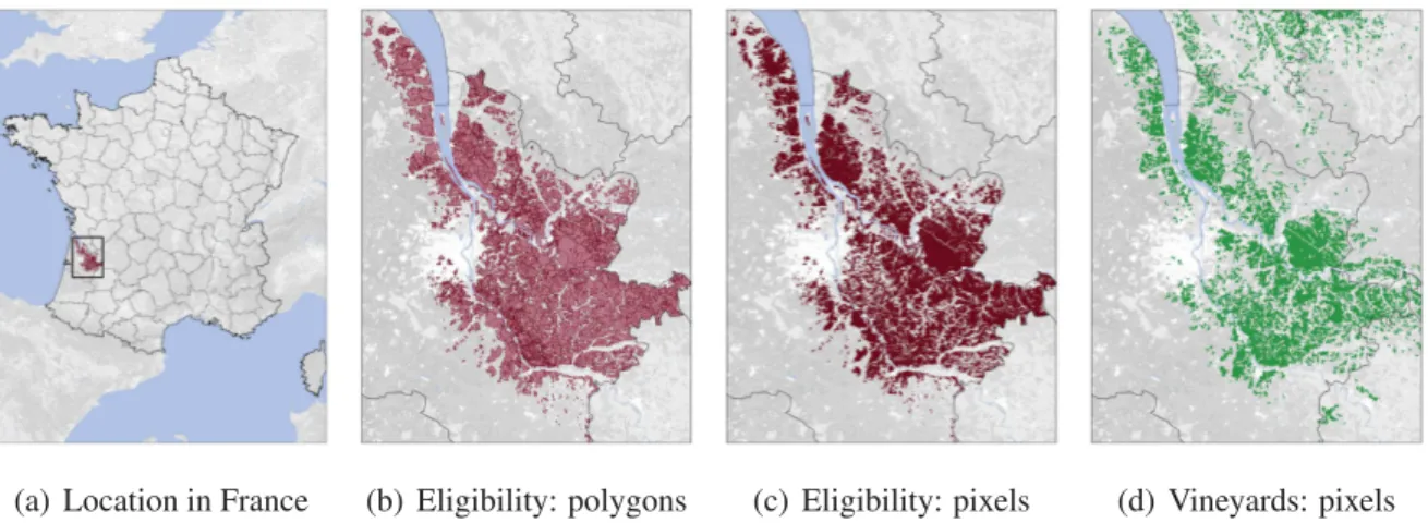
Figure2depicts the selection of the eligible area for the AOC bordeaux, entirely located within the Gironde department. Panel (b) depicts the polygon file from INAO, showing the contours of the eligible area. Panel (c) shows the pixelation of the eligible area, and panel (c) shows the pixels planted in vineyards from the land use dataset. The intersection of the areas selected in panels (c) and (d) represents our measure of the eligible vineyard area.
To construct the share of vineyards eligible for AOC recognition at the level of a department, our unit of analysis, we divide the area eligible for at least one AOC (while being grown in vineyards) in the department by the maximum of the area planted in vineyards during the period 1907–1969, which comes directly from the historical record in the Statistique agricole annuelle. This calculated share represents our best estimate of the historical share of eligible vineyards. For each AOC, we use the year following the year of enactment of the decree as the starting date for counting AOC eligibility.
(a) Location in France (b) Eligibility: polygons (c) Eligibility: pixels (d) Vineyards: pixels
Figure 2: The area eligible for the bordeaux AOC
Formally, denote by i a department, by m a municipality, by t a year, by l an AOC, and by p a one-hectare pixel. Let us further denote:
1lmt =
1 if municipality m is eligible for AOC l per regulation in force in year t 0 otherwise 1lp =
1 if AOC l is not covered by the 2019 INAO map
or if pixel p belongs to AOC l per the 2019 INAO map
or if pixel p belongs to a municipality m not eligible for AOC l per the 2019 INAO map
0 otherwise
1p =
1 if pixel p was grown in vineyards in 1990, 2000, 2006, 2012, or 2018 0 otherwise
.
Given that we start counting recognition in the year following an AOC decree, the indicator 1lmt equals zero from 1907 until the year in which a decree for AOC l is enacted that includes
municipality m as eligible, and one thereafter. If m is excluded from that AOC by a modifying decree enacted during the sample period, the change is assumed to take place the year following the publication of the modifying decree.
Denoting by m(p) the municipality to which belongs pixel p, we also define Npt=ql1lm(p)t1lp1p
as the number of distinct AOCs for which pixel p was eligible in year t.29 Denoting byΣ
isthe
area in vineyards (under production or not) in department i in year s and by P(i) the set of pixels in department i, we construct our main regressor as
skit ≡
q
p∈P(i)1Npt≥k
maxsΣis
which indicates the share of department i’s vineyards eligible for k or more AOCs as of year t. Our main set of regressions only use s1it, the share of vineyards eligible for at least one AOC, but in AppendixCwe also consider s3itand s5itin order to investigate whether prices are influenced by the number of AOCs that an area can claim. For five departments largely covered by broad regional AOCs, our proxy of the acreage eligible for at least one AOC eventually becomes greater than the maximum area in vineyards over the sample period.30 In these cases, we set the
share of eligible acreage equal to one.
29
In doing so, we do not double-count AOCs recognizing different colors of wine. For instance, if a parcel is eligible for producing both red and white AOC wine, we only count one AOC, the idea being that a given wine can only be sold under one color. As a result, the multiplicity of AOCs for a given parcel arises solely from the hierarchical structure of the AOC system.
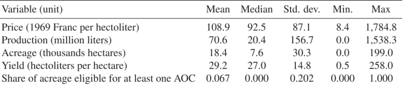
Table 1: Summary statistics
Variable (unit) Mean Median Std. dev. Min. Max
Price (1969 Franc per hectoliter) 108.9 92.5 87.1 8.4 1,784.8
Production (million liters) 70.6 20.4 156.7 0.0 1,538.3
Acreage (thousands hectares) 18.4 7.6 30.3 0.0 199.0
Yield (hectoliters per hectare) 29.2 27.0 14.8 0.5 258.0
Share of acreage eligible for at least one AOC 0.067 0.000 0.202 0.000 1.000
Lastly, we verify that our proxy is consistent with the AOC production data reported in the Statistique agricole annuelle from 1942 onwards. For three departments, we find the share of eligible acreage to be unreasonably small relative to the share of AOC production. We correct these shares using ancillary data on current AOC acreage reported in the 2010 edition of the French wine guide Guide Hachette.31 Conversely, four departments with a nonzero eligible
acreage yet report zero AOC wine production. We can rationalize these discrepancies, however. Three of them are only eligible for the brandy AOCs cognac and armagnac, for which the corresponding wine production is not reported as AOC (perhaps because the AOC is granted to the final liqueur but not to the wine itself). The fourth one is Haute-Marne, where only two municipalities are eligible for the AOC champagne. The AOC production in this department was thus either very small and neglected in the reports or reported in an adjacent department. Table 1 shows summary statistics for a set of variables relevant to our analysis, including the eligible vineyard shares s1it, s3it, and s5it. Figure 3 depicts the temporal rollout of AOC recog-nitions and, whenever available, the national vineyard area under AOC and the national AOC wine production.32
31Our algorithm yields an eligible acreage share equal to zero in Ain and Haute-Savoie, although both
de-partments report a small AOC production. This is because the AOC seyssel, which has eligible parcels in these departments, has no pixel planted in vineyards in the land use data. For Pyrénées-Atlantiques, our algorithm at-tributes a share of eligible acreage more than three times smaller than the share of AOC production. One possibility is that AOC yields are three times larger than non-AOC yields in that department (and even more if not all eligible producers comply), which is doubtful. A more likely explanation is that the AOC jurançon has too few planted pixels in the land cover data (only 1% of the eligible pixels are reported as planted in vines). Since seyssel and jurançon are still produced in non-negligible volumes today, the satellite imagery clearly fails to identify all pixels in vines in the regions covered by these appellations, perhaps due to their relatively high altitude and the declivity of the terrain. Hence, we use the average cultivated acreage reported in the wine guide, which leads to shares of eligible acreage (respectively 0.3, 1.1 and 9.3% for Ain, Haute-Savoie, and Pyrénées-Atlantiques) that are in line with the average shares of AOC production (respectively 0.3%, 3.8%, and 6.0%) over the available years. An alternative correction strategy is to consider all eligible pixels in the INAO maps as being planted, which leads to qualitatively identical regression estimates. Our results also hold when using the data without any correction and when excluding these three departments. Finally, Isère, a department located in the Alps, reports an infinitesimal AOC wine production, however we failed to find any official AOC in use in this department. Our results are robust to the exclusion of that department.
32The vineyard area under AOC was obtained from estimates reported in INAO (1978) and corresponds to
(a) Cumulative distribution (b) Share in France total
Figure 3: Temporal rollout of AOC recognitions and AOC production
Notes: The count of decrees represented in this figure includes the 34 Burgundy premiers crus created in 1943 but excludes the 577 climats relative to these premiers crus. Similarly, it excludes the 64 municipality names which can be attached to the AOCs beaujolais and mâcon. All these appellations are duly accounted for in the econometric analysis as additional layers.
5. Analysis
We begin with a discussion of our strategy to identify the effect of the reform on wine prices and assess its statistical significance. We then present our empirical results, including the effect on the average wine price, its interpretability in terms of quality improvements, and an estimate of the AOC price premium.
5.1. Identification strategy
We exploit two sources of variation to identify the effects of the reform on the average wine price: variation in the exposure of a department to the reform (through its eligible share of vineyards) and variation in the timing of the decrees taken in application of the 1935 law. Most decrees were enacted during the years 1936 and 1937, although several were adopted later, notably those pertaining to the Alsace region in 1962. Importantly, the reform affected wine-producing departments unevenly: many had no AOC area, some had complete AOC eligibility, and many had only a share of their vineyards recognized as eligible. This cross-sectional vari-ation provides both an extensive and an intensive margin of treatment that allows us to control for common shocks to departmental wine prices through year fixed effects.
One concern when assessing the effect of a program or rule on outcomes is that implementation is not exogenous, i.e. rules happen to be implemented concurrently with other factors affect-ing the outcome. For instance, if appellation decrees happen to be in force at the same time
Figure 4: Definition of vignobles
Notes: Delineations in light gray represent departments. Delineations in black represent vignobles. Hatched departments are excluded from the analysis because they produced little to no wine during the period.
that demand factors, say expanding export markets, are affecting wine prices, then the effect of foreign demand might be mistakenly attributed to regulation if it happens to affect treated and untreated departments differently. Our strategy to control for such potentially confounding fac-tors is to further differentiate the year fixed effects by vignoble, that is, the broad geographical area that defines wines, such as “Loire” or “Midi.” To define these vignobles, we largely follow the classification adopted by INAO, making sure that each vignoble is large enough to include at least a couple of departments, our cross-sectional units of analysis. Our dataset includes 16 vignobles and 76 departments, depicted in Figure4.
Formally, our preferred specification can be spelled out as follows:
log pit = αi+ γvt+ β′sit+ δ′xit+ ǫit (4)
where i denotes a department, t denotes a year, v denotes the unique vignoble to which depart-ment i belongs, pit is the average price of wine in department i in year t, αi is a department
fixed effect, γvt is a vignoble-by-year fixed effect, xitis a vector of quantity controls, and sitis
a vector of treatment variables capturing the extent of AOC recognition in department i in year
t. For instance, the vector sitmay include the share of a department’s vineyard acreage eligible
in year t for one or more and three or more AOCs. The vector β captures the effects of interest. We include controls for quantity produced, either in year t or in year t − 1, because wine production is highly dependent on weather. Indeed, departmental output displays wide fluctua-tions from year to year (see Figure 5). These fluctuations are not due to planting decisions, as vineyard acreage has moved smoothly over time, but rather to yield effects channeled through weather shocks. Conditional on vignoble-by-year fixed effects, output variations can therefore be considered exogenous to price, and we thus interpret Equation (4) as an (inverse) demand
(a) Wine output (b) Productive acreage
Figure 5: Wine output and productive acreage in AOC and non-AOC departments
Notes: Areas exclude departments with missing data. AOC departments (23) have a 1969 share of vineyards eligible for AOC larger than 20%. Non-AOC departments (32) have a 1969 share of vineyards eligible for AOC smaller than 2.5%. Departments with an intermediate share (11) not represented.
equation.33 The coefficient δ represents the (derived) demand flexibility for wine at the
depart-mental level. The coefficient β represents the shift in marginal willingness to pay for wine, conditional on output. Note that removing quantity controls from the regression will not quali-tatively change our estimate of β.
Our identifying assumption is that within a vignoble, treated and untreated departments would have followed parallel price movements after the AOC reform if not for the reform itself. Given the limited geographical span of our vignobles, we find it unlikely that remaining unobservables correlated with the AOC share within a vignoble-year could confound the effect of regulation. Controlling for vignoble-by-year fixed effects means that our identification relies on differences, within a vignoble, in the share of vineyards eligible for an AOC in a given year following the reform. Such differences arise from different shares of a department’s vineyard area being eligi-ble for a given appellation and, to a lesser extent, from different dates of adoption of decrees for different appellations. For instance, if two departments in the same vignoble are only eligible for one and the same appellation, they will nonetheless participate in identification as long as they have different shares of vineyards eligible for that appellation. Conversely, if two depart-ments in the same vignoble have the same share eligible, but this share relates to two distinct appellations with decrees taken at different dates, they will participate in identification as well. Assuming that decree adoption does cause an increase in wine prices, we expect departments within a vignoble with larger shares of vineyards eligible to have higher price increments upon AOC recognition; we also expect eligible departments within a vignoble to experience price increases sooner if their decrees are enacted sooner. Violation of our identification assumption would require the existence of unobservable factors systematically correlated with AOC status
33
Milhau(1948,1949) uses a similar argument and a similar regression to identify the demand for wine during the period 1919–1933 at the national level, treating aggregate realized output as exogenous to price.
within a vignoble in the many years we observe following the reform. In support of our identi-fication assumption, we use 30 years of pre-reform data to rule out such systematic differences across departments with differing eventual AOC status.
5.2. Inference
Our specification includes vignoble-by-year fixed effects. These fixed effects flexibility con-trol for annual shocks common to departments located in the same vignoble, notably those due to weather shocks that could affect quality independently of quantity (which is explicitly con-trolled for). On average, there are fewer than five departments in each vignoble. Our preferred standard errors assume that, conditional on these geographically differentiated yearly shocks and other included regressors, there is no residual correlation in errors across departments. Nonetheless, we allow for serial correlation across years within a department through the use of department-level clusters. We believe that this is important because we observe outcomes in many years, and treatment is correlated across years before and after the reform. We view department-clustered standard errors as conservative enough, particularly given the small num-ber of departments within each vignoble.34 Further, because we sample all departments in all
vignobles, there is no sampling design justification for clustering at the vignoble level (there are no relevant vignobles absent from our data set that we wish to draw inference about). In-stead, we view our sampling as occurring in the time dimension, in which case department-level clusters should be appropriate (Abadie et al.,2017).
For comparison purposes, we also report two other types of standard errors: (i) standard errors computed using the method of Conley(1999) adapted for panel data,35and (ii) standard errors clustered at the level of a vignoble. Unlike the department- and vignoble-clustered standard errors, Conley errors do not account for serial correlation of the error term.
5.3. Results
Before discussing our main results and considering competing explanations for the observed price effect, we present suggestive evidence that AOC recognition positively affected the tra-jectory of wine prices at the department level. A detailed heterogeneity analysis is provided in AppendixC.
34As a point of comparison,Jensen and Miller(2008) report standard errors clustered at the level of the treatment
unit (a household) in a panel regression that includes county-by-year fixed effects, even though the number of households per county in their study is 100–150.
35
The Conley errors are to spatial data what West errors are to time-series data. We apply the Newey-West weighting scheme to neighboring relationships when calculating our standard errors.
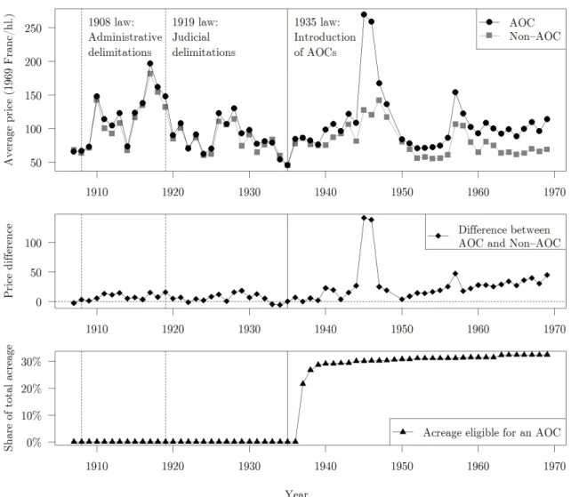
Figure 6: Average real wine prices in AOC and non-AOC departments
Notes: Average real wine prices are calculated using production weights and conditioning on departments with-out missing data. Prices deflated by CPI. Production weights are constant over time and calculated as the average departmental wine production over the pre-reform period from 1907 to 1936. AOC departments (23) have a 1969 share of vineyards eligible for AOC larger than 20%. Non-AOC departments (29) have a 1969 share of vineyards eligible for AOC smaller than 2.5%. Departments with an intermediate share (11) not represented.
5.3.1. Suggestive evidence
The top panel of Figure6plots a time-series of average real wine prices across two categories of departments: those with high eventual AOC share (with an eligible share of AOC vineyards larger than 20% by 1969) and those with low eventual AOC share (with an eligible share lower than 2.5%). A few departments with intermediate share are not represented. The middle panel of the figure plots the evolution of the difference between the two averages, and the bottom panel shows the evolution of the share of acreage eligible to an AOC.
Figure6shows that the two categories of departments had very similar prices before the AOC reform, even after the appellation laws of 1908 and 1919 were passed. The two price series only start to diverge after the AOC reform, with higher values in departments with high eventual AOC
(a) Price trend (b) AOC share (c) Correlation
Figure 7: Trends in departmental real wine prices over the period 1907-1969
Notes: Price trends are computed using changes in 25-year averages from the endpoints of the period and are expressed in relative terms. The share of vineyards eligible for AOC is calculated as of 1969. White departments: no data available.
share, particularly in the immediate aftermath of WWII.36As depicted in the bottom panel, the
implementation of the 1935 law only started with the first set of AOC decrees published in 1936, which we consider affected the eligible acreage, in practice, one year later.
The figure provides visual support for the “parallel trends” assumption implicit in difference-in-differences designs.37 What the figure does not capture, but our main regression will, is any
differential price trends within the two broad categories defined here according to the AOC eligible share and the behavior of prices in departments with intermediate share (that is, the intensive margin of treatment along the AOC share dimension), as well as the fact that recogni-tion did not happen simultaneously in all treated departments (the intensive margin of treatment along the time dimension).
Figure 7 depicts trends in real wine prices over the period 1907 to 1969 at the departmental level, using changes in 25-year averages from the endpoints of the period to compute the rel-ative increase in price. It also depicts the share of vineyards eligible for AOC recognition by department as of 1969. Qualitatively, Figure7tells a similar story as the previous figure: price trends over the period 1907-1969 appear to be stronger in departments with higher AOC shares. One may be worried that departments with eventually high shares of AOC recognition may have been on a steeper price trend for reasons unrelated to regulation. For instance, one could perhaps imagine that producers in departments with steeper price trends lobbied harder for AOC recognition. To investigate this possibility, we compare two simple price trend regressions based on different subsamples of years: 1907–1936 (pre-reform) and 1927–1956 (pre-post-reform), where price trends are computed using 10-year averages from the endpoints of each period and
36In a robustness check, we show that our estimates are not driven by data from that period. See Table9. 37Average prices in the departments with intermediate eventual AOC share do not contradict this story: prices in
those departments were consistently below those in non-AOC departments before the reform, and caught up after it.
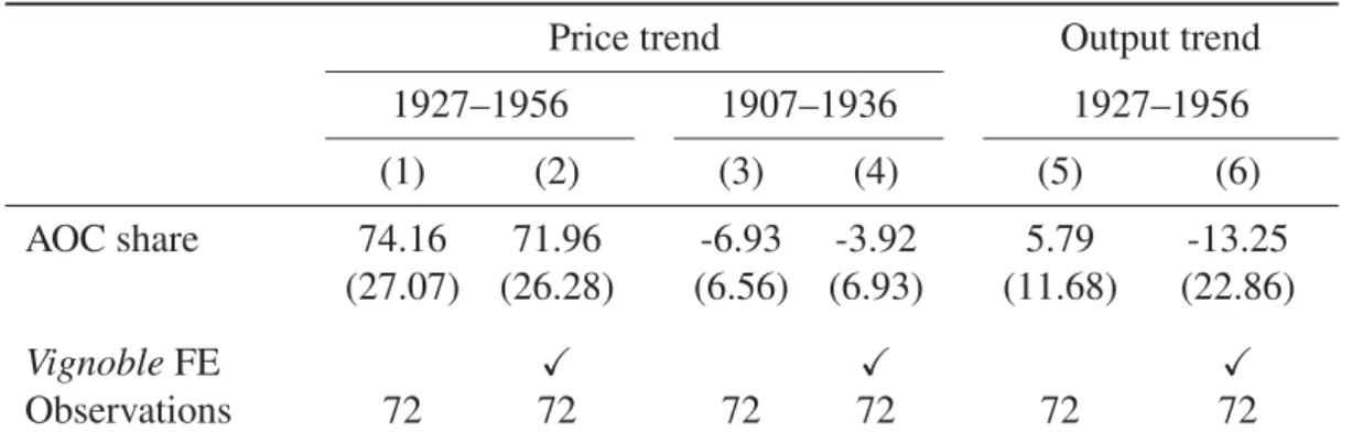
Table 2: Trends regressions
Price trend Output trend
1927–1956 1907–1936 1927–1956 (1) (2) (3) (4) (5) (6) AOC share 74.16 71.96 -6.93 -3.92 5.79 -13.25 (27.07) (26.28) (6.56) (6.93) (11.68) (22.86) Vignoble FE X X X Observations 72 72 72 72 72 72
Notes: The sample is limited to departments with enough information to compute price and output trends over the two periods 1907–1936 and 1927–1956. Heteroskedasticity-robust standard errors are reported in brackets. The vignoble control includes 16 different wine regions.
are expressed in relative terms. The results are reported in Table 2. Column (1) of the table reports the coefficient on the AOC eligible share (by 1956) from a regression of the price trend calculated over the period 1927–1956. Column (2) controls for vignoble to purge the regression of effects common to all departments located in the same wine region. In both columns, the coefficient on the AOC share is highly significant, suggesting that AOC eligibility had a positive effect on price trends, even after controlling for vignoble effects. In contrast, columns (3) and (4) show that if we focus on price trends during the pre-reform period, the AOC share does not have any explanatory power, that is, eventual AOC eligibility (as of 1956) is irrelevant to explaining price trends prior to regulation. Finally, columns (5) and (6) show that AOC eligibility also had no clear effect on wine output, suggesting that the effects of regulation on price trends were not the result of a reduction in volumes.
5.3.2. Panel analysis
The results from the estimation of Equation (4) appear in Table3and Appendix TablesB.1and
B.2. Each table uses a different window of time to identify the effects of AOC recognition, from the widest (1907–1969, the entire data set) to the narrowest (1921–1950). We show results with different sets of controls. Every regression includes department and year fixed effects. Except for column (6), all columns control for production in some way. For a given time window, estimates of the effect of the AOC eligibility share are quite similar across specifications, even when omitting production controls.
We do not necessarily expect coefficient estimates to be stable across time windows. One ba-sic reason is that as periods change, so does the set of appellations that are recognized in the sample. For instance, appellations in the Alsace region were recognized relatively late, in 1962. Because AOC recognition may cause different price increases in different regions, our coef-ficient estimate, which captures an average effect, may vary according to the period used. In