HAL Id: hal-02893190
https://hal.telecom-paris.fr/hal-02893190
Submitted on 8 Jul 2020
HAL is a multi-disciplinary open access
archive for the deposit and dissemination of
sci-entific research documents, whether they are
pub-lished or not. The documents may come from
teaching and research institutions in France or
abroad, or from public or private research centers.
L’archive ouverte pluridisciplinaire HAL, est
destinée au dépôt et à la diffusion de documents
scientifiques de niveau recherche, publiés ou non,
émanant des établissements d’enseignement et de
recherche français ou étrangers, des laboratoires
publics ou privés.
Daniel Knorreck, Ludovic Apvrille, Renaud Pacalet
To cite this version:
Daniel Knorreck, Ludovic Apvrille, Renaud Pacalet. Fast Simulation Techniques for Design Space
Exploration. International Conference on Objects, Components, Models and Patterns (TOOLS
EU-ROPE 2009), 2009, Zurich, Switzerland. �hal-02893190�
Exploration
Daniel Knorreck, Ludovic Apvrille, and Renaud Pacalet
System-on-Chip Laboratory (LabSoC), Institut Telecom, Telecom ParisTech, LTCI CNRS, 2229, Routes des Crˆetes BP 193 F-06904 Sophia Antipolis, France {daniel.knorreck,ludovic.apvrille,renaud.pacalet}@telecom-paristech.fr
Abstract. This paper addresses a UML based toolkit for performing efficient system-level design space exploration of System-On-Chip. An innovative simulation strategy to significantly reduce simulation time is introduced. The basic idea is to take benefit from high level descriptions of applications by processing transactions spanning potentially hundreds of clock cycles as a whole. When a need for inter task synchronization arises, transactions may be split into smaller chunks. The simulation en-gine is therefore predictive and supports backward execution thanks to transaction truncation. Thus, simulation granularity adapts automati-cally to application requirements. This paper also highlights the benefits of TTool, an open-source toolkit that fully integrates the aforementioned simulation engine. Emphasis is more particularly put on procedures tak-ing place under the hood after havtak-ing pushed the simulation button of the tool. Finally, the new simulation strategy is assessed and compared to an earlier cycle-based version of the simulation engine.
Key words: System-On-Chip, Design Space Exploration, System Level Modeling, UML, DIPLODOCUS, TTool, Fast Simulation Techniques
1 Introduction
System-level design space exploration in a System-on-Chip (SoC) design cy-cle is an issue of great concern in today’s rapidly growing and heavily con-strained design processes. The increasing complexity of SoC requires a complete re-examination of design and validation methods prior to final implementation. We believe that the solution to this problem lies in developing an abstract model of the system intended for design, on which fast simulations and static formal analysis could be performed in order to test the satisfiability of both functional and non functional requirements.
In this context, we have previously introduced a UML-based environment named DIPLODOCUS. The strength of our approach relies on formal verification ca-pabilities and fast simulation techniques ( [16] [4]).
DIPLODOCUS design approach is based on the following fundamental princi-ples:
– Use of a high level language (UML)
– Clear separation between application and architectural matters – Data abstraction.
– Use of fast simulation and static formal analysis techniques, both at applica-tion and mapping levels
The designer is supposed to model in an orthogonal fashion the application and the architecture of the targeted system. Thereafter, a mapping stage associates application and architectural components. As mentioned initially, simulation is an integral part of the DIPLODOCUS methodology and enables the designer to get first estimates of the performance of the final system. In that context, an important issue to solve is the concurrency of operations performed on hard-ware nodes and more particularly on CPUs and buses. The first version of our simulation environment relied on the standard SystemC kernel and took advan-tage of the integrated discrete event simulator. Further information about this approach can be found in [10]. In that simulator, a SystemC process is assigned to each active hardware node, and a global SystemC clock is used as a means of synchronization. Abstract communication and computation transactions defined in the application model are broken down to the corresponding number of wait cycles. Thus, all active components are run in lockstep.
Unfortunately, the inherent latency of the SystemC scheduler due to frequent task switches made the simulation su↵er from low performance. However, simula-tion speed is an issue of concern as it represents one argument to justify accuracy penalties as a result of abstractions applied to the model. In order to achieve a better performance, a new simulation strategy is presented in the scope of this paper. It leverages these abstractions by processing high-level instructions as a whole whenever possible. Furthermore, its simulation kernel incorporates a slim discrete event scheduler so that SystemC libraries are not necessary any more. The paper is composed of seven sections. Section 2 gives an overview of our methodology and points out the features of the integrated development environ-ment TTool. Section 3 introduces the main concepts of the simulation strategy and illustrates them with a concrete example. Section 4 provides an insight into algorithmic issues and explains the significance of transactions and the time stamp mechanism for fast simulation. Furthermore, the simulation procedure is structured in terms of phases and synchronization issues are tackled which arise when tasks exchange data and events. Section 5 benchmarks the new simulation engine and compares its performance to the previous simulator version. Section 6 compares our approach with related works. Section 7 finally concludes the paper and draws perspectives.
2 The DIPLODOCUS Environment
DIPLODOCUS is a UML profile targeting the design of System-on-Chip at a high level of abstraction. A UML profile customizes UML [9] for a given domain, using UML extension capabilities. Also, a UML profile commonly provides a methodology and is supported by a specific toolkit.
2.1 Methodology
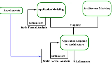
DIPLODOCUS includes the following 3-step methodology (see Figure 1): 1. Applications are first described as a network of abstract communicating
tasks using a UML class diagram. Each task behavior is described with a UML activity diagram.
2. Targeted architectures are modeled independently from applications as a set of interconnected abstract hardware nodes. UML components have been defined to model those nodes (e.g. CPUs, buses, memories, hardware accelerators, bridges).
3. A mapping process defines how application tasks can be bound to execution entities and also how abstract communications between tasks are assigned to communication and storage devices.
Application Modeling
Simulations Static Formal Analysis
Architecture Modeling Requirements
...
Application Mapping on Architecture Mapping SimulationsStatic Formal Analysis Refinements
Fig. 1. Global view of our Design Space Exploration Approach
A task activity diagram is built upon the following operators: control flow and variable manipulation operators (loops, tests, assignments, etc.), communication operators (reading/writing abstract data samples in channels, sending/receiving events and requests), and of computational cost operators.
One main DIPLODOCUS objective is to help designers to find a hardware archi-tecture that satisfies functional and non-functional requirements. To achieve this,
DIPLODOCUS relies on fast simulation and formal proof techniques. The appli-cation models are designed independently of targeted underlying architectures. Due to the high abstraction level of both application and architecture, simu-lation speed can be increased significantly with regards to simusimu-lations usually performed at lower abstraction level (e.g. TLM level, RTL level, etc.). Addition-ally, efficient static formal analysis techniques may be applied before and after mapping.
Within a SoC design flow, Design Space Exploration is supposed to be carried out at a very early stage, right after a specification document has been issued. In the scope of hardware/software partitioning, several appropriate architectures could be assessed by means of our methodology. Thus, it should be emphasized that DIPLODOCUS designs are settled above more detailed but still abstract models like TLM. Indeed, the main di↵erence between DIPLODOCUS and TLM models relies in data (and not only signal) abstraction and the modeling of com-putational complexity. Hence, with DIPLODOCUS, a designer can already get a first estimate of the behavior of final applications even if some algorithmic details have not yet been stipulated.
2.2 Application modeling in a nutshell
An application model is the description of functions to be performed by the targeted SoC. As mentioned before, functions are modeled as a set of abstract tasks described within UML class diagrams. One has to bear in mind that, at application modeling level, there is no notion of time but only a partial ordering between actions. This section briefly describes a subset of TML (Task Modeling Language) instructions as well as their semantics and provides definitions for Channels, Events and Requests:
– Channels are characterized by a point-to-point communication between two tasks. The following Channel types exist:
– Blocking Read-Blocking Write (BR-BW) – Blocking Read-Non Blocking Write (BR-NBW) – Non Blocking Read-Non Blocking Write (NBR-NBW)
– Events are characterized by a point-to-point unidirectional asynchronous communication between two tasks. Events are stored in an intermediate FIFO between the sender and the receiver. This FIFO may be finite or infinite. In case of an infinite FIFO, the incoming events will never be lost. In case of a finite FIFO, adding a new event to a full FIFO removes the oldest. Thus, a single element FIFO may be used to model hardware interrupts. In TML tasks, events can be sent (NOTIFY), received (WAIT) and tested for their presence (NOTIFIED).
– Requests are characterized by a multi-point to one point unidirectional asyn-chronous communication between two tasks. A unique infinite FIFO between
senders and the receiver is used to store all incoming requests. Consequently, no request may be lost.
The behavior of abstract tasks it specified by means of TML which is based on UML Activity diagrams. As some of the constituting operators are referred to in later sections, a brief survey is provided which is not meant to be exhaustive:
Icon: Command: Semantics:
READ x Read x samples in a channel WRITE x Write x samples in a channel NOTIFY e Notify event e with 3 parameters WAIT e Wait for event e carrying 3 parameters REQUEST Ask the associated task to run
EXECI x Computational complexity of x execution units Table 1. TML Commands
2.3 Toolkit
The DIPLODOCUS UML profile - including its methodology - has been im-plemented in TTool [1]. TTool is an open-source toolkit that supports several UML2 / SysML profiles, including TURTLE [3] and DIPLODOCUS [2]. The main idea behind TTool is that all modeling may be formally verified or sim-ulated. In practice, UML diagrams are first automatically translated into an intermediate specification expressed in formal language, which serves as starting point for deriving formal code and simulation code.
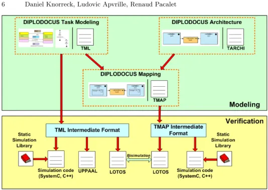
TTool has the following main modeling capabilities (see Figure 2):
– Modeling of applications using either a UML class diagram or a specific language called TML. From both formats, it is possible to generate simulation code or formal verification specifications from which formal proofs may be performed.
– Modeling of architectures using UML deployment diagrams (or a textual format named TARCHI).
– Modeling of mappings using UML deployment diagrams (or a textual for-mat named TMAP). A mapping scheme associates applications and tures. Based on these three building blocks (mapping, application, architec-ture), TTool automatically generates simulation code or formal specifications at the push of a button.
Fig. 2. Modeling and verification capabilities of TTool
From DIPLODOCUS application or mapping models, TTool may perform sim-ulations or formal proofs:
– For simulation purpose, TTool generates SystemC or C++ code. Indeed, TTool is currently equipped with two simulators: one based on the SystemC simulation engine, and another and more recent one implemented in pure C++. That generated code is linked with libraries - included in TTool - be-fore being executed. Also, The C++-based simulator is the main contribution described later on in the paper. This C++ simulator outperforms its SystemC counterpart in terms of simulation speed, but it is yet not compatible with third-parties SystemC-based components.
– For formal proof purpose, TTool generates LOTOS or UPPAAL code. Formal verification of application or mapping models is out-of-scope of this paper. Before being translated into either SystemC, UPPAAL or LOTOS, models are first translated into intermediate languages. Figure 2 refers to this process. In this paper, emphasis is put on post-mapping simulation of tasks mapped onto a given hardware architecture. More precisely, we introduce our new simulation scheme. It is indeed especially suited to exploit characteristics of our high level task and architecture descriptions. The two next sections of the paper are more particularly focused on the architecture of the simulation engine, and on its performance.
3 Introducing fast simulation techniques
3.1 Basic principles
The simulator detailed in this paper is transaction-based. A transaction refers to a computation internal to a task, or a communication between tasks. Those transactions may obviously last from one to hundreds of clock cycles. Transac-tion duraTransac-tions are initially defined according to the applicaTransac-tion model, that is to say their maximum duration is given by the length of corresponding operators within tasks description. At simulation runtime, a transaction may have to be broken down into several chunks of smaller size, just because for example, a bus is not accessible and so the task is put on I/O wait on its CPU. Transaction cutting is more likely to happen when the amount of inter task communication is high and hence the need for synchronization arises.
Unlike a conventional simulation strategy where all tasks are running in lockstep, a local simulation clock is assigned to each active hardware component. Thus, simulation granularity automatically adapts to application requirements as ab-stract measures for computational, and communicational costs of operations are specified within the application model. The coarse granularity of the high level description is exploited in order to increase simulation speed.
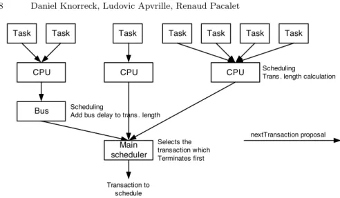
A problem at stake when considering transaction-based simulation is the schedul-ing of transactions themselves. This procedure embraces mainly four elements (see Figure 3): tasks, CPUs, buses and the main scheduler. The sequence of the entities of the aforementioned list also reflects their hierarchy during the schedul-ing process: tasks are settled at the top layer and the main scheduler constitutes the lowermost layer. Based on the knowledge of their internal behavior, tasks are able to determine the next operation which has to be executed within their scope. This operation is encapsulated subsequently in a transaction data struc-ture and forwarded consecutively to hardware components being in charge of its execution.
The basic idea is that a transaction carries timing information taken into account by hardware components to update their internal clock. Moreover, a hardware component may delay transactions and modify their duration according to the execution time needed by that specific component. By so doing, the simulation algorithm accounts for the speed of CPUs, the data rate of buses, bus contention and other parameters characterizing the hardware configuration.
More precisely, on time management, tasks tag each transaction with its earliest start time (which is equal to the finish time of their previously executed transac-tion) and an abstract measure of the computational complexity or of the amount of data to transfer respectively. CPUs in turn have to recalculate the start time based on their internal schedule and are able to convert the abstract length to time units. Buses are in charge of handling communication transactions which are treated in a similar way. If several devices are involved in the execution process, transactions are simply passed from one device to another device and
Task Task Task CPU Bus Task Task Task Task CPU CPU Main scheduler nextTransaction proposal Scheduling
Trans . length calculation
Scheduling
Add bus delay to trans . length
Transaction to schedule
Selects the transaction which Terminates first
Fig. 3. Object collaboration during scheduling process
modified accordingly. Correct values for start time and duration are hence de-termined incrementally by forwarding transactions to dedicated hardware nodes. Finally, the main scheduler acts as a discrete event simulator and assures the causality of the simulation.
3.2 Example illustrating the Main Scheduler
To illustrate the cooperation of entities discussed previously and the main sched-uler, we consider the following example:
The notion of transaction refers to a portion of a command. A READ command for instance allows for an inter task communication by reading a given number of samples from an abstract channel. For example let us consider the expression READ 3. This command could be broken down into two transactions, the first one reading one sample and the second one reading the two remaining samples. The basic idea is to try at first to schedule a transaction having the same length as the command (3 in our example). If the attempt fails, the transaction is sub-sequently split into smaller parts which can be scheduled. We first suppose that the command can be executed as a whole. The command is subdivided into sev-eral transactions if another transaction interferes with the first one.
That way the simulation overhead decreases if the amount of inter task depen-dency is low. The worst case of that approach is when scheduling policies of CPUs and buses are based on a strict alternation between tasks: in that case, the simulation environment gets back to a cycle based simulation because every transaction is automatically reduced to the length of 1. This scenario could be avoided with the aid of bus scheduling policies relying on atomic burst transfers which cannot be interrupted.
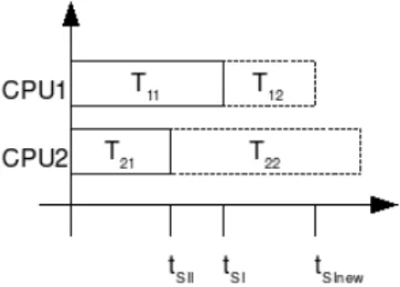
As an more complex example, let us consider the scenario depicted on Figure 4: there are two CPUs, referred to as CPU1 and CPU2. A CPU model merges both an abstract hardware component and an abstract real time operating system. Both CPUs (CPU1 and CPU2) have already executed a transaction of a task T11 and T21 respectively. The transaction on CPU1 finished at tSI, the one on
CPU2 finished at tSII. The schedulers of both CPUs subsequently propose the
next transaction to execute. The simulation algorithm selects the transaction which will terminate first because its execution could have an impact on other tasks (making them runnable for instance). This decision is in line with tradi-tional mechanisms used for discrete event simulation. As we have to be sure that during the execution of the selected transaction no events will occur, special care has to be taken when considering communication-related commands (read to channel, write to channel, wait on event, notify event, ...). The length of these transactions are therefore calculated based on the number of samples to read, the number of samples to write, the content and the size of the channel as well as the size of atomic burst transfers on the bus.
After T12 has been scheduled, tSI is set to the end time of T12, referred to as
tSInew. If the completed transaction T12 causes a task to become runnable on
CPU2, T22is truncated at tSInewand the remaining transaction is scheduled on
CPU2. As a channel always links only two tasks, revealing dependencies becomes trivial. If a portion of T22has been added to the schedule, tSIIis changed
accord-ingly (tSII= tSInew). After this, all schedulers of CPUs which have executed a
transaction are invoked. The algorithm has now reached its initial state where all schedulers have selected a potential next transaction. Again, the transaction which finishes first is scheduled...
4 Algorithmic details
4.1 Transactions and the timestamp policy
This chapter elaborates on the attributes which characterize transactions. One has to discern two time scales within a transaction: a virtual one and an absolute one. The virtual time scale bases on the number of execution units (for com-mands modeling computational complexity) and the amount of data to transfer (READ/WRITE commands for abstract channels) respectively. Thus, the vir-tual time scale does not depend on architecture specific parameters (such as the speed/data rate of devices). The absolute time is calculated as a function of the virtual time and device parameters.
The performance of a real application may su↵er from penalties caused by hard-ware components and the operating system. Since those delays strongly impact the runtime behavior of applications, transactions also account for lost cycles. In line with the granularity of our simulation, penalties are randomly determined on a per-transaction base. That means that the exact point in time when a penalty occurs within a transaction is not resolved. All lost cycles are added to the payload of a transaction and they are displayed at the beginning of a transaction in simulation traces. This display format has been chosen arbitrarily and any other format would be just as appropriate.
The main attributes of a transaction are tabulated below:
– startTime: Stands for the absolute point in time when the transaction starts – length: Indicates the number of time units needed to execute the transaction – virtualLength: Specifies the amount of data to read/write or the amount of processing units to carry out (example: for a READ 3 and a channel having a width of 2, the corresponding transaction spanning the whole operation would have a virtualLength of 6)
– runnableTime: Indicates the point in time when the transaction gets runnable, it is determined by the dedicated task
– idlePenalty: If a CPU has no more instructions to execute, it enters idle mode after a given delay. Tasks requesting CPU processing time may su↵er from the wake-up delay of the CPU. This behavior is modeled with the aid of the idle penalty. The delay is not neglectable for embedded systems attempting to achieve a moderate power consumption.
– taskSwitchingPenalty: The scheduling service of an OS also accounts for a cost in terms of processing time. Furthermore, the context of tasks (regis-ters,...) has to be saved in the memory.
– branchingPenalty: Pipelined CPU architectures entail lost cycles due to so called pipeline-flushes. If a branch has not been predicted correctly, some partially executed commands have to be discarded. This delay is referred to as branching penalty.
As stated in the introductory part of this paper, timestamps contained in trans-actions are exploited by hardware components as well as by the main scheduler.
This paragraph elaborates on the contribution of each entity which modifies transactions - including commands and channels which have not been intro-duced yet. Transactions are initiated by commands as the latter keep track of their internal progress. Our modeling methodology provides abstract channels which have their representation within the simulation environment. Di↵erent se-mantics like Blocking Read-Blocking Write, Non Blocking Read-Non Blocking Write and Blocking Read-Non Blocking Write have to be respected. Each object depicted in Figure 5 is thus able to (re)calculate one or more transaction at-tribute(s) based on its internal state. Arrows denote the data flow of transaction pointers.
1. TMLCommand initially instantiates a transaction. The amount of remaining processing units (the di↵erence between the virtualLength of the command and its progress) is assigned to virtualLength. Furthermore, a first estimate of the runnableTime is stored in the dedicated variable. The value simply amounts to the time when the last transaction of the command terminated. 2. Due to its inner state (i.e. filling level, references to transaction attempting to read/write,...), a channel is able to deduce the definite value of runnable-Time. The time determined by the command is delayed if the channel is blocked due to an overflow or an underflow of data. TMLChannel recalcu-lates virtualLength depending on the value proposed by TMLCommand and the content and the size of the channel (a detailed description of this pro-cedure given later in this paper). In other words: a channel may truncate a transaction if its inner state does not allow for executing the transaction as a whole.
3. The CPU class finally computes the start time of the transaction and its real duration. To determine the startTime, runnableTime has to be deferred to the end of the schedule (EndLastScheduledTransaction). The absolute length of a transaction depends on the product of the processor frequency and virtualLength as well as on possible task penalties. If the objective of the transaction is a bus transfer, length is calculated within the bus class. 4. This last step is only carried out for transactions necessitating bus access.
Possibly startTime is delayed once again due to bus contention and the real length of a transaction is calculated based on the bus frequency.
4.2 Simulation phases
The simulation algorithm is structured such that each command has to be pre-pared before it is able to execute. Thus, simulation enters alternately prepare and execution phases of commands. When the simulator is launched initially, the first command of each task is prepared. During simulation, it is sufficient to prepare only those commands which have executed a transaction.
At the end of the prepare phase, transactions which might be processed by CPUs are known, only bus scheduling decisions are pending. That way, the prepare phase is crucial for the causality of the simulation.
Fig. 5. Data flow of a transaction
Following tasks are accomplished during the prepare phase:
1. It has to be checked if the current command has been processed entirely. In this case, the progress of the command is equal to its virtual length and the following command is activated.
2. The number of remaining virtual execution units is calculated. 3. A new transaction object is instantiated.
4. If the concerned command tends to read/write samples from/in channels, it has to be checked if the current state of the channel permits this operation. Therefore, read and write transactions are registered at the channel. 5. Task variables may be evaluated or modified.
The objective of the execution phase is to update state variables of the simulation after a transaction has been carried out. To achieve this, the following actions have to be taken:
1. Issue read/write operations on channels definitely so that state variables of channels are updated.
2. Update the progress of a command achieved by a completed transaction. 3. Add transactions to the schedule of CPUs and buses.
Now, the basic phases have been introduced and attention should be drawn to the way they are arranged to conduct the simulation procedure:
1. At first, the prepare phase of the the first command of all tasks is entered. 2. Schedulers of all CPUs are invoked to determine the next transaction. Each
CPU may have its own scheduling algorithm.
3. CPU schedulers register their current transaction at the appropriate bus in case the transaction needs bus access.
4. The main scheduler is in charge of identifying the runnable transaction t1
which may check in turn if bus access was granted for their communication transaction. Bus scheduling is triggered in a lazy manner when the scheduling decision is required by CPUs.
5. The execution phase for transaction t1 is entered.
6. If transaction t1 makes another task T runnable which is in turn able to
execute a new transaction t3, transaction t2 currently running on the CPU
on which T is mapped is truncated at the end time of transaction t1. The
execution phase t2is entered. During the next scheduling round, the
sched-uler of the aforementioned CPU is able to decide whether to switch to t3or
to resume t2.
7. Commands which have been executing are prepared. 8. CPUs which have carried out a transaction are rescheduled. 9. Return to step 3
4.3 Synchronization issues
The virtualLength of a transaction has to be calculated carefully: the result strongly impacts the scheduling process. When a transaction has been sched-uled definitely, it is impossible to return to the past to add preemption points. This design decision has been taken in favor of simulation performance. Un-fortunately, this convention imposes that the next preemption point has to be anticipated at the time when transaction parameters are determined. Commands which tend to synchronize tasks by transferring data via channels are especially critical. To address this issue, let us examine the algorithm which determines the virtualLength of WRITE and READ transactions.
A blocking channel is meant to establish a synchronization between a READ and a WRITE transaction (and vice versa). Thus virtualLength of READ/WRITE transactions has to be updated when the transaction is registered at the chan-nel(preparation phase) and when a transaction is executed (execution phase). The example given hereafter illustrates the situation:
1. Transaction 1 is registered during a preparation phase, its virtualLength is computed.
2. Transaction 2 is registered in a subsequent preparation phase, its virtual-Length is determined, virtualvirtual-Length of transaction 1 is updated.
3. When either of these two transactions is executed, virtualLength of the re-maining transaction is updated.
4. The last transaction is executed.
The reader might wonder why four calculations are carried instead of two (one for each transaction). The reason for this is that the channel has no knowledge about the order in which the two transactions will be executed. Furthermore, as we will see in following, the number of samples to read (if any) depends on the number of samples to write (if any) and vice versa. This fact implies that the attributes of transaction 1 must be recalculated upon registration of transaction 2 as well as upon its execution.
In accordance with previous observations, one can infer an adequate algorithm for calculating the length of a WRITE transaction:
1. If there is no read request, the length of a WRITE transaction is limited by the minimum of the number of samples to write and the free space in the channel.
2. If there exists a read request and the channel holds enough samples to satisfy the demand right away, the limiting factors are the same as above.
3. If there exists a read request and the channel does not hold enough data to satisfy the demand, there is an additional limiting factor as compared to the cases above: the number of samples which have to be written so that the READ command can be executed. In other words: the task attempting to read could wake up due to a WRITE executed previously.
The algorithm for READ transactions is derived in an analogous manner: 1. If there is no write request, the length of a READ transaction is limited
by the minimum of the number of samples to read and the content of the channel.
2. If there exists a write request and the channel has enough free space to satisfy the demand right away, the limiting factors are the same as above. 3. If there exists a write request and the channel does not have enough free space
to satisfy the demand, there is an additional limiting factor as compared to the cases above: the number of samples which have to be read so that the WRITE command can be executed. In other words: the task attempting to write could wake up due to a READ executed previously.
A limiting factor has been introduced which is intended to establish additional preemption points after a given amount of data has been transferred. It is re-ferred to as burst size and is considered as the size of a non-preemptive bus transaction. In an extreme case where burst size=1, two tasks alternately write and read one sample.
5 Experimental results
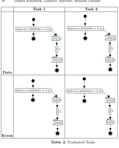
Two important cases are considered to evaluate the performance of our simula-tion engine: event notificasimula-tion/recepsimula-tion on the one hand and communicasimula-tion via a data channel on the other hand. Therefore, task sets depicted in table 2 have been executed on both simulators - the SystemC one, and the C++ one - and the execution time has been captured. The measurements have been performed under the following conditions:
1. Output capabilities of both simulators are disabled in order to measure the pure simulation time. No trace files are created.
2. The time consumed by the initialization procedure of both simulation envi-ronments is not taken into account for the same reason.
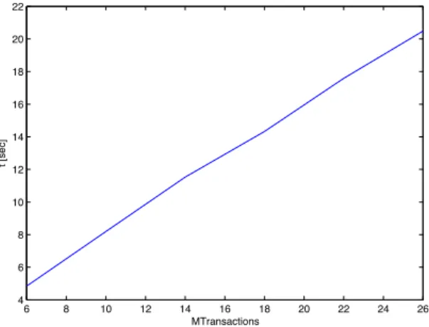
3. All measurements are subject to noise caused by the multi tasking operation system and interfering tasks running on the same CPU. Therefore, the aver-age of several measured values has been taken into account for all di↵erent tests. Thus the noise should distort similarly the results for both simulators. 4. As the analysis has been carried out on a less powerful machine, only the comparison of both simulators is meaningful in Figures 6 and 7, and not the absolute execution times. According to this, Figure 8 merely reflects the qualitative behavior of the new simulator; it performs much faster on recent machines.
The first task set is composed of two tasks communicating by means of a Block-ing Read-BlockBlock-ing Write channel with the width parameter set to 1 and the length parameter set to 100. All commands are nested in a 1 million-loop struc-ture. This way, the ratio of execution time of the simulator and noise due to the multitasking operating system (task switches,...) is increased.
Let us now have a closer look at the example tasks. Task 1 writes x samples into channel ch1, performs x integer operations and finally reads x samples from channel ch2. Task 2 carries out the complementary operations, it reads x samples from channel ch1, performs x integer operations and writes x samples to chan-nel ch2. The second task set is configured similarly: the only di↵erence is that channels are replaced by events based on infinite FIFOs. Figure 6 and Figure 7 depict the execution time as a function of x which varies from 1 to 10.
It can be deduced that the execution time of the old simulator grows more or less linearly with the command length. For the new simulator however, the execution time does not depend on the command length as one command corresponds to one transaction in this simulation. The execution time of the new simulator is only impacted by the number of transactions (linear growth, see Figure 8). But even in the worst case, when all transactions have a length of 1, the new sim-ulator outperforms the old version by approximately a factor of 10. Depending on the respective model, the gain can be much higher given that a transaction comprises several cycles. Thus, the new simulator automatically adapts to the granularity of the application model: if a task issues commands having a length of one cycle, the simulator falls back on a cycle based consideration. If transactions are long, simulation efficiency increases accordingly.
Task 1 Task 2
Data
Event
Table 2. Evaluated Tasks
1 2 3 4 5 6 7 8 9 10 0 10 20 30 40 50 60 70 command length time [sec] Old simulator New simulator
1 2 3 4 5 6 7 8 9 10 0 10 20 30 40 50 60 70 command length time [sec] Old simulator New simulator
Fig. 7. Event performance for old and new simulator
6 8 10 12 14 16 18 20 22 24 26 4 6 8 10 12 14 16 18 20 22 MTransactions t [sec]
6 Related work
There are many approaches in practice today which tackle the Design Space Ex-ploration issue. In the following, a few of the most relevant and widely practiced approaches are discussed very briefly. Some of the key features and limitations are highlighted and a comparison with our approach is provided:
The Ptolemy environment [8] is based on a simulator that o↵ers di↵erent lev-els of abstraction for jointly simulating - or verifying - hardware and software components. Ptolemy is rather focused on embedded systems than specifically on design space exploration.
In POLIS environment, applications are described as a network of Codesign Fi-nite State Machines (CFSMs) [6]. Each element in the network can be mapped onto either a hardware or a software entity. This approach di↵ers from our work because it deals with application models mainly and there is no separation of architecture and application models. However, it is also intended for formal anal-ysis.
Metropolis is a design environment for heterogeneous systems [5]. It o↵ers var-ious models of computation (MoCs). However, both application and architecture are modeled in the same environment. It uses an Instruction Set Simulator (ISS) to generate execution traces which relies on executable application code. Hence, there is no abstraction at application level.
In SPADE/SESAME, applications are modeled as Kahn Process Networks (KPN) which are mapped onto the architecture models and the performance is analyzed through simulation [11] [12] . There is separation of application and architecture. This approach utilizes symbolic instructions (abstractions of RISC instructions) and the models are not generic.
In ArchAn (Architecture Simulation Environment), the architecture is modeled at the cycle-accurate level using a mixture of synchronous language Esterel and C. ArchAn focuses on the optimization of hardware architecture by early per-formance analysis [14] [7]. However the approach in ArchAn does not describe the application and architecture in an orthogonal fashion. It is not intended for formal analysis as well.
[15] proposes a methodology to speed up simulations of multi-processor SoCs at TLM level with additional timing information. The idea of time propagation through transaction passing bears some resemblance with our new simulation approach. However, our environment is settled at a higher abstraction level so that the procedure of transaction passing has been extended to optimally sup-port high level models. As our aim is fast simulation, our simulation engine is not based on the SystemC kernel any more.
[13] also follows the Y-Chart approach. Mapping of applications to architec-tures is performed on graph-based descriptions and based on side-information provided by the system designer. The mapping methodology uses abstract in-formation such as cycle counts, and as opposed to our approach the control flow of algorithms cannot be refined. The aforementioned framework is not intended for formal analysis.
7 Conclusions and future work
The main contribution introduced in the paper is the description of a lightweight discrete event simulation engine which is especially optimized for DIPLODOCUS high level application models. Simulation granularity is automatically adapted to the requirements of the application thanks to our transaction-based approach. When experimenting with models such the one of an MPEG2 decoder, we experi-enced performance gains in terms of execution time up to factor 30 as compared to a cycle-based SystemC simulator. It should be reemphasized that the gain depends on the application model, it could potentially be much higher.
Several improvements are currently under development.
At first, hardware components model could be enhanced. For example, the bus model shall reflect modern communication architectures comprising several pos-sible communication paths (e.g. Network-on-Chip). The memory model is cur-rently merely based on a fixed latency. Furthermore, latency due to bu↵ers in buses and bridges has been omitted. Thus, model realism versus simulation com-plexity is still under study for hardware components. Second, we expect to per-form profiling of our simulation engine so as to identify time-consuming sections of code and recode them (e.g. in assembly language). Also, multiprocessor / core architectures could improve simulation performance significantly.
At last, more advanced simulation capabilities shall be introduced. Indeed, we expect the simulation engine to be able, at run-time, to check for functional requirements (e.g. if a client requests the bus, access is granted within 10ms). Also, it would also be very interesting to automatically explore several branches of control flow in order to enhance the coverage of simulations.
References
1. Ttool, the turtle toolkit: http://labsoc.comelec.enst.fr/turtle.
2. L. Apvrille. TTool for DIPLODOCUS: An Environment for Design Space Ex-ploration. In Proceedings of the 8th Annual International Conference on New Technologies of Distributed Systems (NOTERE’2008), Lyon, France, June 2008. 3. L. Apvrille, P. de Saqui-Sannes, R. Pacalet, and A. Apvrille. Un environnement
UML pour la conception de systmes distribus . Annales des Tlcommunications, 61:11/12:1347–1368, Novembre 2006.
4. L. Apvrille, W. Muhammad, R. Ameur-Boulifa, S. Coudert, and R. Pacalet. A uml-based environment for system design space exploration. Electronics, Circuits and Systems, 2006. ICECS ’06. 13th IEEE International Conference on, pages 1272–1275, Dec. 2006.
5. F. Balarin, Y. Watanabe, H. Hsieh, L. Lavagno, C. Passerone, and A. Sangiovanni-Vincentelli. Metropolis: an integrated electronic system design environment. Com-puter, 36(4):45–52, April 2003.
6. Felice Balarin, Massimiliano Chiodo, Paolo Giusto, Harry Hsieh, Attila Jurecska, Luciano Lavagno, Claudio Passerone, Alberto Sangiovanni-Vincentelli, Ellen Sen-tovich, Kei Suzuki, and Bassam Tabbara. Hardware-software co-design of embedded systems: the POLIS approach. Kluwer Academic Publishers, Norwell, MA, USA, 1997.
7. A. Chatelain, Y. Mathys, G. Placido, A. La Rosa, and L. Lavagno. High-level architectural co-simulation using esterel and c. Hardware/Software Codesign, 2001. CODES 2001. Proceedings of the Ninth International Symposium on, pages 189– 194, 2001.
8. J. Eker, J.W. Janneck, E.A. Lee, Jie Liu, Xiaojun Liu, J. Ludvig, S. Neuendorf-fer, S. Sachs, and Yuhong Xiong. Taming heterogeneity - the ptolemy approach. Proceedings of the IEEE, 91(1):127–144, Jan 2003.
9. Object Management Group. UML 2.0 Superstructure Specification. In http://www.omg.org/docs/ptc/03-08-02.pdf, Geneva, 2003.
10. Ludovic Apvrille Muhammad Khurram Bhatti. Modeling and simulation of soc hardware architecture for design space exploration. October 2007.
11. A. D. Pimentel, S. Polstra, and F. Terpstra. Towards efficient design space ex-ploration of heterogeneous embedded media systems. In In Embedded Processor Design Challenges: Systems, Architectures, Modeling, and Simulation, pages 57–73. Springer, LNCS, 2002.
12. A.D. Pimentel, C. Erbas, and S. Polstra. A systematic approach to exploring embedded system architectures at multiple abstraction levels. Computers, IEEE Transactions on, 55(2):99–112, Feb. 2006.
13. Bastian Ristau, Torsten Limberg, and Gerhard Fettweis. A mapping framework for guided design space exploration of heterogeneous mp-socs. Design, Automation and Test in Europe, 2008. DATE ’08, pages 780–783, March 2008.
14. M. Silbermintz, A. Sahar, L. Peled, M. Anschel, E. Watralov, H. Miller, and E. Weisberger. Soc modeling methodology for architectural exploration and soft-ware development. Electronics, Circuits and Systems, 2004. ICECS 2004. Pro-ceedings of the 2004 11th IEEE International Conference on, pages 383–386, Dec. 2004.
15. E. Viaud, F. Pecheux, and A. Greiner. An efficient tlm/t modeling and simula-tion environment based on conservative parallel discrete event principles. Design, Automation and Test in Europe, 2006. DATE ’06. Proceedings, 1:1–6, March 2006. 16. M. Waseem, L. Apvrille, R. Ameur-Boulifa, S. Coudert, and R. Pacalet. Abstract application modeling for system design space exploration. Digital System Design: Architectures, Methods and Tools, 2006. DSD 2006. 9th EUROMICRO Conference on, pages 331–337, 0-0 2006.