Longitudinal effects of an optic nerve injury on visual behaviour

(1)

(2)

Université de Montréal

Longitudinal Effects of an Optic Nerve Injury on Visual

Behaviour

Effets longitudinaux d’un écrasement du nerf optique sur le

comportement visuel

par Jacqueline Higgins

École d’optométrie

Mémoire présenté en vue de l’obtention du grade de Maîtrise en Sciences de la vision,

option Sciences fondamentales, appliquées et cliniques

juin 2019

(3)

Résumé

Une maladie ou un traumatisme du système visuel peut avoir des conséquences à long terme sur la vision. Cependant, des études récentes ont examiné la plasticité cérébrale comme moyen de restaurer une vision fonctionnelle malgré les dommages. Pour mieux comprendre l'implication de la plasticité et de la réorganisation neuronale suite à un déficit, ce mémoire étudie la récupération spontanée des fonctions visuelles par des tests comportementaux chez la souris. L’écrasement partiel du nerf optique (pONC), permettant une vision résiduelle, a été induit selon deux intensités. Les tests comportementaux des fonctions visuelles incluaient le réflexe optomoteur, qui mesure le réflexe du suivi visuel de la souris en réponse à un réseau sinusoïdal, ainsi que le test de la falaise visuelle qui évalue la perception de profondeur. Ces tests ont été effectués une fois avant le pONC, puis à plusieurs moments jusqu'à 28 jours post-opération. La survie des cellules ganglionnaires rétiniennes donnant naissance au nerf optique a ensuite été quantifiée. Les résultats ont montré qu’un pONC de haute intensité entraînait une cécité et une perte de la perception de profondeur, sans amélioration dans les 28 jours suivants, tandis qu’un pONC de faible intensité permettait une récupération partielle des deux paramètres. La perte des cellules rétiniennes était plus forte pour le pONC de haute intensité, surtout dans les régions proximales. Ces résultats montrent une récupération spontanée des fonctions visuelles, à part si le dommage cellulaire est trop important.

(4)

Abstract

Disease or trauma to the visual system can cause long-term damage and severe visual deficits. However, recent research has turned to neural plasticity as a means to recover functional vision despite anatomical damage. To understand the involvement of neural plasticity and reorganization following a deficit, the present thesis investigated the spontaneous recovery of visual functions over time using behavioural tests in mice. Specifically, a partial optic nerve crush (pONC) was induced with two injury intensities, while still allowing for residual vision from surviving retinal cells. Behavioural assessments of visual functions included the optomotor reflex test, which measured the mouse’s tracking reflex in response to moving sinusoidal gratings, while the visual cliff test evaluated depth avoidance behaviour by simulating a cliff to observe the animal’s perception of depth. The tests were performed once before the injury, then at multiple time points up to 28 days. Retinal ganglion cell survival was subsequently quantified. Results showed that the high-intensity pONC led to a complete loss of visual acuity and depth avoidance, with no improvement in the following 28 days, whereas the low-intensity pONC showed a partial recovery. There were fewer surviving cells after the high-intensity pONC, especially in proximal regions. These results show evidence of spontaneous recovery of visual functions, but only with a certain amount of cell survival.

(5)

List of Figures

Figure 1. Visual field defects. ... 3

Figure 2. Axonal degeneration. ... 4

Figure 3. Layers of the retina. ... 7

Figure 4. The optic nerve. ... 10

Figure 5. Projections from the retina to the primary and secondary visual pathways. ... 12

Figure 6. The accessory optic system of the mouse. ... 14

Figure 7. Possible axonal outcomes following injury to the optic nerve. ... 17

Figure 8. Forceps used to perform a partial optic nerve crush. ... 21

Figure 9. Timeline of experiments. ... 21

Figure 10. Optomotor reflex test. ... 23

Figure 11. Visual cliff test. ... 24

Figure 12. Changes in visual acuity over time, as measured by the optomotor reflex test. 28 Figure 13. Changes in depth perception over time, as measured by the visual cliff test. ... 29

(8)

List of Acronyms and Abbreviations

AOS: Accessory Optic System

CDEA: Comité de déontologie de l’expérimentation sur les animaux CERNEC: Centre de recherche en neuropsychologie et cognition CNS: Central Nervous System

CRIR: Centre de recherche interdisciplinaire en réadaptation du Montréal métropolitain dLGN: dorsal Lateral Geniculate Nucleus

DTN: Dorsal Terminal Nucleus

INLB: Institut Nazareth et Louis Braille IQR: Interquartile Range

LP: Lateral Posterior nucleus MTN: Medial Terminal Nucleus NOT: Nucleus of the Optic Tract OKR: Optokinetic Reflex

OPM: Olivary Pretectal Nucleus pONC: partial Optic Nerve Crush

RBPMS: RNA-Binding Protein with Multiple Splicing RF: Receptive Field

RGC: Retinal Ganglion Cell SC: Superior Colliculus

SCN: Suprachiasmatic Nucleus V1: Primary Visual Cortex VA: Visual Acuity

(9)

(10)

Acknowledgments

First, I would like to thank my graduate supervisor Dr. Elvire Vaucher for accepting me into her lab, and for her guidance and support throughout my master’s degree. Thank you for showing me the different facets of fundamental and clinical research, and for giving me the opportunity to collaborate with such a wide variety of professionals in the field. Thank you to Marianne for being such an incredible mentor and friend, thank you for having the patience to teach me and answer my millions of questions. I could not have done this without you both!

Many thanks to the members of the lab, both past and present. Thank you to Brenda and Jérôme for showing me around the city and helping me with my very first experiments. Thank you to Guillaume and Marie-Charlotte for helping me through stressful days, but also celebrating the good ones. I am so grateful to call you my friends and colleagues. Thank you Soumaya, Rahmeh, Michèle, and Visou for your support, you always know how to make me laugh. Thank you to my friends and colleagues in the school of optometry. Thank you to Bruno for all of your help with the OptoMotry system and immunofluorescence. You are a great teacher! Thank you to Geneviève for your guidance and advice, I always know I can come to for answers.

In addition, I would like to thank the members of my thesis jury for agreeing to evaluate my graduate research. I would also like to thank l’Université de Montréal, l’École d’optométrie, le Centre de recherche en neuropsychologie et cognition (CERNEC), Institut Nazareth et Louis-Braille (INLB), and the Vision Health Research Network (VHRN) for their financial support.

Lastly, I would like to thank my parents for their love and support, and Justin for his patience, kindness, and understanding. Justin, thank you for believing in me and supporting me, I know the submission of this thesis is just as exciting for you as it is for me!

(11)

Introduction

Humans are a highly visual species. Though perceiving the world around us seems simple and natural, our visual system is, in reality, extremely complex. In fact, more than one third of the human cerebral cortex is dedicated to visual processes (Bear, Connors, & Paradiso, 2016). We rely on vision to perceive, navigate, and adapt to our environment. However, when the visual system is affected by trauma, ocular disease or an alteration of the cortical visual system (e.g. stroke or cancer), it often leads to devastating vision loss. The population affected by a visual deficit continues to increase dramatically, with approximately 36 million individuals who are blind and 216.6 million individuals with moderate to severe visual impairment worldwide (Bourne et al., 2017).

Prevalent causes of visual impairment include cataracts, age-related macular degeneration, diabetic retinopathy, and glaucoma (Congdon et al., 2004; Roodhooft, 2002). These ocular diseases, affecting the eye and optic disc, have long been the focus of our understanding of visual impairment. With ocular diseases, cortical processing within the brain remains relatively intact, and the visual stimuli are simply not received by the cells in the eye and, consequently, the brain (Martin et al., 2016). However, when damage occurs at the level of transmission and/or processing in the brain, this typically leads to perceptual deficits that have more complex consequences yet to be fully understood (Dutton, 2003). These neurological deficits of the visual system are the primary focus of the present thesis as they cause devastating vision loss with very few treatment options available. In order to treat such deficits, it is important to first understand the progression of the deficit and then potentialize the mechanisms of recovery. To this end, rodents have become increasingly popular models for studying visual deficits and recovery, as used in the present study.

1. Visual Field Defects

Both ocular and neurological visual impairments are classified by the severity of visual acuity (VA) and/or visual field loss. VA is a measure of spatial resolution or the smallest detectable stimulus, while visual field is the area in which a stimulus can be detected. An

(12)

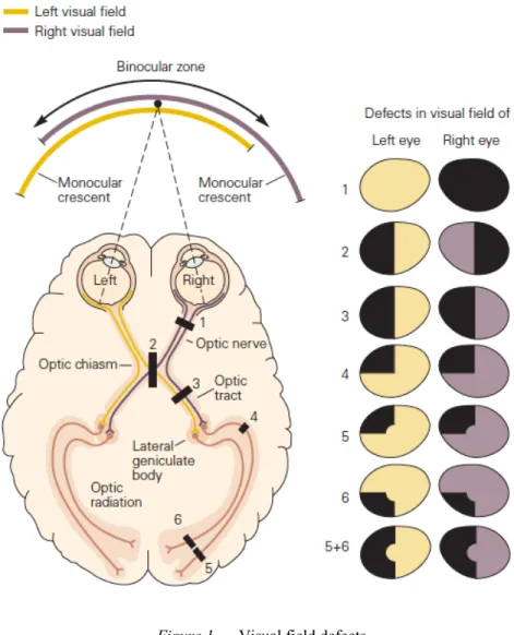
individual is considered blind if they have a best corrected VA of worse than 3/60 or a visual field of less than 10° in the better eye (Roodhooft, 2002). Visual field defects arise from disease, stroke, or trauma affecting a structure somewhere along the primary visual pathway, and can impair daily activity performance and quality of life (Ajina & Kennard, 2012). The effects of the deficit on the visual field and related visual functions are dependent on the extent and location of the injury (Chokron, Perez, & Peyrin, 2016) (Fig. 1). The loss of visual field can be only a few degrees of the field of view (scotoma), a quarter of the field of view (quadranopia), a hemifield (hemianopia) or the entire field of view for that eye (optic nerve damage). These visual field deficits lead to problems in visual acuity, contrast sensitivity, colour vision, as well as oculomotor skills and visual perception.

(13)

Figure 1. Visual field defects.

Characteristics of visual field defects (shaded sections of the visual field representations to the right) depend on the position of the lesion or injury along the visual pathway (labeled black rectangles in the left diagram, which represents the ventral view of the brain and optic pathways) (figure from Kandel, Schwartz, Jessell, Siegelbaum, & Hudspeth, 2013).

1.1. Optic Nerve Injuries

Disease or injury to the optic nerve greatly affects the input of the visual scene to the brain, resulting in altered visual processing and visual fields defects (Fig. 1). The optic nerve is composed of the axons of retinal ganglion cells (RGCs), the neurons in the retina that project to the brain. Optic nerve damage primarily results from 1) acute traumatic injury/traumatic optic

(14)

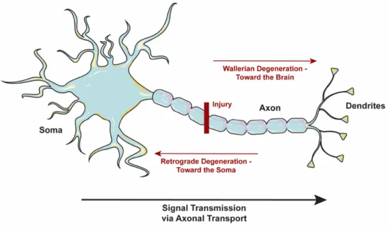
neuropathy (Benowitz & Yin, 2010), 2) benign or malignant tumours compressing the optic nerve (Miller, 2004), 3) glaucoma, a disease characterized by an increase in intraocular pressure which can subsequently cause damage to the optic nerve head (Benowitz & Yin, 2010) or 4) multiple sclerosis, which can result in optic neuritis via inflammatory deterioration of the nerve’s myelin sheath (Manogaran et al., 2018). Many other conditions and factors can also contribute to optic nerve damage (e.g. hypoplasia, medications). Damage to the optic nerve results in extensive retrograde RGC death across the retina (Sabel, 1999). Similar to other neural cells, RGCs affected by various types of stressors (including physical damage to the cell axons) undergo degeneration, loss of function, and ultimately cell death via apoptosis. Specifically, damage to the optic nerve causes both retrograde and Wallerian degeneration of the RGC axons that extend toward the RGC layer of the retina and the brain, respectively (Kanamori, Catrinescu, Belisle, Costantino, & Levin, 2012) (Fig. 2). There is also evidence of a second degenerative phase, in which RGCs with damaged axons will negatively affect the surrounding RGCs, though this is still unclear (Nickells, 2012).

Figure 2. Axonal degeneration.

Damage to a neural axon results in retrograde degeneration (damage extending towards the soma) or Wallerian degeneration (damage extending toward the dendrites). In the case of RGC axon injuries, Wallerian degeneration leads to loss of signaling to the brain as neural signals are transmitted through the axon (neuron outline CC BY Servier Medical Art).

(15)

As a result of physical damage, optic nerve injuries result in long-term loss of functional vision (de Lima et al., 2012). Optic nerve damage may result in visual field loss, VA loss, impairment of colour vision, and occasionally a relative afferent pupillary defect (Jang, 2018; Kumaran, Sundar, & Chye, 2015), depending on the cerebral region affected by this denervation.

2. Recovery of Vision

These visual field defects result in lasting vision loss with devastating consequences on physical and emotional health. However, the visual system is unique, adapting and changing depending on our experiences. This is partly because our visual system is capable of cortical plasticity, based on the reorganization of neuronal networks. This plasticity reflects memory processes or perceptual learning, leading to experience-dependent changes in perception (Gilbert & Li, 2012). What if the visual system could adapt and change in response to a deficit? Recent research has turned its focus to the role of plasticity on visual field deficit recovery and rehabilitation.

2.1. Plasticity and Recovery of Visual Field Defects

Plasticity in the Central Nervous System (CNS) has long been a topic of interest. At the beginning of the 20th_{century, researchers believed that the CNS was not capable of changing or}

adapting. Santiago Ramon y Cajal, a renowned neuroscientist, described the CNS as “fixed and immutable” (Ramon y Cajal, 1928). However, in recent years there has been a shift in perspective, as scientists began to acknowledge the existence of neural plasticity. There are many ways the CNS can adapt, including changes in cognitive strategies for compensation, recruitment of other neurons, changes in the strength of communication between specific neurons, and even changes in cellular structure or synaptic properties (Sharma, Classen, & Cohen, 2013).

Post-lesion neural plasticity and behavioural recovery have been extensively studied due to their potential clinical implications. As the visual system is highly organized and plays a critical role in behaviour, it has often been used to study plasticity and recovery following

(16)

damage to the CNS. In the past decade or so, mice have become increasingly popular models for studying the underlying mechanisms of visual plasticity. Though mice have a very low spatial resolution (Prusky & Douglas, 2004), they provide abundant opportunities for genetic manipulation and circuit labeling, while also being conveniently small, easy to maintain, and relatively cost effective (Huberman & Niell, 2011). In addition, mice have a life-span of approximately 2 years, and therefore develop at a much faster rate than primates, making them a convenient model for longitudinal studies on regeneration (Levkovitch-Verbin, 2004).

3. The Mouse Visual System

The visual system is a complex network in the CNS that processes sensory stimuli from a visual scene. The visual system is composed of neurons, specialized cells that form connections from the eye’s retina to visual regions of the brain. Though this system differs greatly between species, the constructive nature of the primary visual pathway remains, i.e. images are constructed from individual photons transduced into neural signals, beginning at the photoreceptor cells in the retina and developing further in the higher visual cortices. Essentially, photons are presented to the photoreceptors, which activates pigment molecules in the photoreceptors, leading to the transduction of photons into neural signals. Retinal cells have specific receptive fields, which represent distinct areas of the visual field. Consequently, the cell will respond by undergoing a signaling change (e.g. excitatory or inhibitory activation) if stimuli appear within the defined area of the receptive field. Once exposed to stimuli, the photoreceptors will transmit to the RGCs via bipolar cells and other mediating cells, which then send the signal via the optic nerve to the brain. The axons forming the optic nerve project to various subcortical nuclei, ultimately signaling to the visual cortex and associative cortices. Each structure involved in visual processing is highly organized and specialized for a particular visual aspect or function.

However, the visual abilities of a species are limited by the eye’s structure and placement, as well as the physiology in terms of spatial and temporal resolution, and even colour vision (Dusenbery, 1992). Therefore, there are some notable differences between human primate and murine visual systems. For example, due to the lateral positioning of the eyes, mice have a very small binocular field of around 40° (Seabrook, Burbridge, Crair, & Huberman,

(17)

2017). Primates, on the other hand, have a very large binocular field of approximately 120° (Stidwill & Fletcher, 2011). Mice also have a reduced VA, with a performance threshold of about 0.5 cpd (cycles per degree) (Prusky, West, & Douglas, 2000), whereas cats have an acuity of about 20 cpd (Clark & Clark, 2013), and humans have an acuity of about 30 cpd (i.e. 20/20). Nevertheless, the mouse is often used as a model for understanding the fundamental mechanisms of visual processing (Huberman & Niell, 2011; Seabrook et al., 2017).

3.1. The Retina

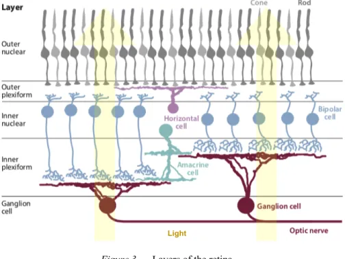
The retina, the innermost layer of the posterior surface of the eye, receives the projections of light refracted off of the cornea and lens. Photons of light are converted into electrophysiological signals and then processed within the various cell layers of the retina according to a specific organization. The retina consists of 5 major types of cells, uniformly distributed across the entire retina, divided throughout 5 principal layers (Fig. 3).

Figure 3. Layers of the retina.

The retina consists of 5 layers: 2 plexiform layers and 3 nuclear layers. When light enters the eye, it is processed via the direct pathway (photoreceptors – bipolar cells – RGCs). The RGCs then transmit information to the brain.

(18)

The amacrine and horizontal cells induce lateral signals in the 2 plexiform layers, modulating the direct pathway (figure adapted from Dhande, Stafford, Lim, & Huberman, 2015).

First, photons penetrate into the retina, attaining the outer nuclear layer where they are received by the photoreceptors. Photoreceptors are the cells that convert the photons of light into neural signals and can be classified into two functional groups based on their sensitivities to certain visual characteristics. Rods are specific to low light (scotopic) conditions, while cones are specific to colour ranges and full light (photopic) conditions. In mice, rods are the predominant photoreceptor, and though they do have cones, they only cover UV to green spectral sensitivities (centered at 360 nm and 511 nm, respectively) (Calderone & Jacobs, 1995). This differs from primates, as humans also have cones for red spectral sensitivities (centered at approximately 560nm) (Berg, Tymoczko, & Stryer, 2002). Neural signals from multiple photoreceptors are then transmitted via bipolar cells to RGCs, the transmission cells that send visual input to the CNS. There is a strong convergence of visual input from the photoreceptors to the bipolar cells, and from the bipolar cells to the RGCs. Therefore, any damage to the RGCs results in a large affected zone of the visual field. Lateral interactions from horizontal and amacrine cells will also modulate this pathway. The interactions between cells results in RGC centre-surround receptive fields. This type of receptive field begins with the bipolar cells, which exist in two types: ON and OFF cells. Generally, light reaching the centre of the receptive field will result in cell activation (ON-centre), while light on the surrounding area results in suppression (OFF-surround). However, there are also OFF-centre ON-surround cells, which result in the opposite effect. In the case of bipolar cells, OFF cells will depolarize in darkness causing an excitatory effect, while ON cells will hyperpolarize in darkness causing an inhibitory effect (Kandel et al., 2013). ON bipolar cells will activate ON RGCs, and OFF bipolar cells will activate OFF RGCs. This partially allows for RGCs to carry out different functions specific to a particular stimulus feature (e.g., contrast, direction of movement, orientation) depending on their type (Baden et al., 2016; Dhande & Huberman, 2014). In the mouse, there are more than 30 types of RGCs, which can be divided into non-direction-selective and direction-selective RGCs (Baden et al., 2016; Huberman & Niell, 2011). For a detailed review on the many different RGC types, see Dhande et al. (2015). All RGCs are ultimately responsible for transmitting the

(19)

signals to the rest of the CNS, as their axons form the optic nerve and project to various areas of the brain. However, there are two predominant RGC projection pathways, mainly processing the principal functions of the retina (i.e. detection of forms, textures, and movements).

3.2. The Optic Nerve

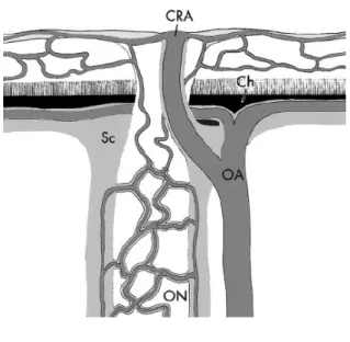
The optic nerve, composed of RGC axons, is the only pathway linking the eyes and the brain. Each optic nerve projects to both cerebral hemispheres, with predominant input to the contralateral hemisphere in mice. The optic nerve originates at the optic disc, and project into the skull until the two nerves merge into the optic chiasm. These projections carry the neural signals generated by the RGC cell bodies, or somas, located throughout the retina of the corresponding eye. In adult C57BL/6J mice, for example, the optic nerve is made up of approximately 45 000 to 55 000 RGC axons (Zarei et al., 2016). In mice, the optic nerve is composed of RGC axons bundled in the center, surrounded by a ring of collagen fibers (May & Lutjen-Drecoll, 2002). The topographic organization of the retina, observed in subsequent cerebral projection regions (i.e. retinotopic organization), is not preserved within the optic nerve. Specifically, the axons exit the eye and form developmentally-ordered fibre bundles until they reach the optic chiasm (Neveu & Jeffery, 2007), where they divide to attain contralateral and ipsilateral brain targets. In humans, RGCs axons in the optic nerve are organized such that contralateral projections are separated from ipsilateral projections and 53% of axons have contralateral projections (Skorkovska, 2017). However, this separation does not exist in the mouse. The organization of RGCs in mice is such that only 5% of projections are ipsilateral, making the axonal projections of the optic nerve mostly contralateral (Seabrook et al., 2017). Similar to primates, the intraocular portion of the optic nerve is not myelinated, meaning there is no myelin sheath to protect and insulate the RGC axons. In fact, myelination of the mouse optic nerve only begins around 0.6-0.8 mm behind the eye (May & Lutjen-Drecoll, 2002). The optic nerve receives its vascular supply from capillaries derived from the central retinal artery, which branches off from the ophthalmic artery that runs next to the optic nerve (outside of the collagen ring), closer to the medial axis (Fig. 4).

(20)

Figure 4. The optic nerve.

Schematic representation of the optic nerve and associated blood supply. Note that the ophthalmic artery is located next to the optic nerve on the medial side (figure from May & Lutjen-Drecoll, 2002). CRA = central retinal artery; Ch = choroid; Sc = sclera; OA = ophthalmic artery; ON = optic nerve.

The RGC axons of the optic nerve project indirectly via synapses along the optic tract and optic radiations to various cortical and subcortical areas. In fact, RGC axons project to over 40 subcortical targets in the brain (Morin & Studholme, 2014). Only a few of these regions are involved in basic visual processing. RGCs mainly form projections to the primary visual structures, notably subcortical nuclei such as the dorsal lateral geniculate nucleus (dLGN) and superior colliculus (SC) which have a role in image forming processes. Other important targets include the suprachiasmatic nucleus (SCN) which regulates circadian synchronicity, the olivary pretectal nucleus (OPN) which controls the pupillary reflex, and the nuclei of the accessory optic system (AOS) which stabilize images on the retina (Seabrook et al., 2017).

3.3. Primary and Secondary Visual Pathways

The axons that form the optic nerve project to complementary image forming areas, organized into the primary and secondary visual pathways. The primary visual pathway involves axonal projections to the dLGN of the thalamus, while the secondary visual pathway involves

(21)

projections to the SC in the midbrain (Fig. 5). These pathways generally maintain the retinotopic representation of the retina (see below). Both pathways continue their projections to various cortical areas, sustaining different visual functions. The dLGN in rodents is relatively homogeneous with no definitive layers, unlike primates, who have distinct cellular layers. However, ipsilateral and contralateral segregation in the dLGN is consistent across species (Seabrook et al., 2017). The dLGN is responsible for integrating and transmitting visual information directly to the primary visual cortex (V1) and many other cortical areas dedicated to conscious visual perception (Huberman & Niell, 2011). The secondary pathway, on the other hand, involves the SC, which is primarily responsible for directing eye and head movements for visual localization. In mice, about 90% of all RGCs project to the SC (Ellis, Gauvain, Sivyer, & Murphy, 2016), which is drastically more than in primates where only about 10% of RGCs project to the SC (Perry & Cowey, 1984). Retinal projections primarily project to the stratum griseum superficialis (SGS), a layer in the SC, which contains a complete retinotopic representation of the contralateral eye (Drager & Hubel, 1976). The deeper layer of the SC, the stratum opticum (SO), contains the retinotopic information from the ipsilateral eye (Drager & Hubel, 1975). The SC sends information to V1 indirectly via the lateral posterior nucleus (LP), known to be involved in modulating attention, and the dLGN.

(22)

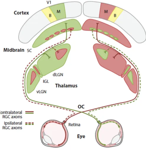
Figure 5. Projections from the retina to the primary and secondary visual pathways.

Retinal ganglion cell (RGC) axons form the two optic nerves, which project to the dorsal lateral geniculate nucleus (dLGN) via the primary visual pathway, and the superior colliculus (SC) via the secondary visual pathway (figure from Seabrook et al., 2017). Other abbreviations include OC = optic chiasm; vLGN = ventral geniculate nucleus; IGL = intergeniculate nucleus; B = binocular zone; M = monocular zone; V1 = primary visual cortex.

3.4. The Primary Visual Cortex

The Primary Visual Cortex (V1), a major portion of the occipital lobe, is essentially a processing hub for visual input. V1 is made up of 6 layers that maintain retinotopic organization and contain a variety of excitatory and inhibitory cell types. Thalamocortical projections from the dLGN project mainly to layer 4 of V1, which consists of a dense layer of excitatory

(23)

pyramidal cells, but some project to layers III and VI. Cells in layer VI then project primarily to layers II and III, but also V and VI to a lesser extent. Thalamocortical projections are divided into two zones in V1: a monocular zone (V1M) and a binocular zone (V1B). Due to the very small binocular visual field in mice, V1M and V1B both receive the majority of their information from the contralateral eye, while V1B receives some information from the ipsilateral eye as well (Fig. 5). This is different from primates and cats, which have distinct ocular dominance columns which alternate between right eye and left eye dominated cortical areas (Seabrook et al., 2017). V1 integrates thalamic inputs and then transmits the relevant information to associative cortical areas, from secondary visual areas to upper cognitive areas (visual hierarchy organization), such as the orbitofrontal cortex. In these associative areas, the organization does not follow the same internal structure as V1. However, lateral connections from other cortical areas are widely present.

3.5. The Accessory Optic System

The AOS is responsible for generating compensatory eye movements in order to properly stabilize a slow-moving image on the retina (Sun et al., 2015). If these movements did not occur, it would result in a retinal slip, causing a blurry perception of the visual scene (Dhande et al., 2015). These eye movements are known as the optokinetic reflex (OKR) and the vestibulo-ocular reflex (VOR). In mice, the accessory optic system is comprised of subtypes of direction-selective RGCs, which target the medial terminal nucleus (MTN), the dorsal terminal nucleus (DTN), and the nucleus of the optic tract (NOT) in the midbrain (Dhande & Huberman, 2014) (Fig. 6). Specifically, projections to the NOT and DTN cause horizontal eye movement reflexes, while projections to the MTN cause vertical eye movement reflexes.

(24)

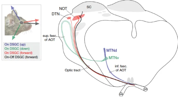
Figure 6. The accessory optic system of the mouse.

Direction-selective retinal ganglion cells (DSGCs) project to various nuclei in the midbrain, depending on the direction of movement, in order to stabilize the image on the retina (figure from Dhande & Huberman, 2014). NOT = nucleus of the optic tract; SC = superior colliculus; DTN = dorsal terminal nucleus; AOT = accessory optic tract; MTNd = dorsal medial terminal nucleus; MTNv = ventral medial terminal nucleus.

3.6. Functional Organization of the Visual System

All regions of the visual system also have a functional organization and contribute to visual perception and resulting behaviours. Functional organization, consisting of specialized neurons with preferential sensitivity interacting with each other through horizontal projections, begins as early as the retina, which receives and transmits every detail of an image. Cone photoreceptors interpret high acuity and high contrast (i.e. difference in luminance or colour) elements, while rods specialize in lower acuity, localization, and movement. This information is transmitted to the RGCs which can be selective in direction, movement, contours, and other visual characteristics (Huberman & Niell, 2011). The vast majority of RGCs then project to either the dLGN (primary visual pathway) or the SC (secondary visual pathway). Though some neurons in both regions encode similar visual information about certain stimuli characteristics

(25)

such as orientation, the dLGN and SC maintain relatively distinct and separate functions dependent on specific visual features. Specifically, the dLGN is responsible for the integration and formation of images and changes in light intensity, while the SC responds primarily to movement (e.g. drifting gratings and moving dots) (Ellis et al., 2016). Parallel processing in these two pathways ultimately projects to V1, which integrates a wide range of signals. Most neurons in V1 are classified by their specificity for orientation or movement. Though V1 processing is mainly contralateral, there is still a substantial amount of binocular integration in V1 (Metin, Godement, & Imbert, 1988). The interactions between these structures result in a variety of subconscious (subcortical) and conscious (V1 and higher cortical areas) visual behaviors.

4. Rodent Model of Optic Nerve Injury

The partial optic nerve crush (pONC) is a model of diffuse axonal injury in rodents which has been extensively used to study the behavioural, physiological, and morphological consequences of an afferent visual deficit (Rousseau & Sabel, 2001). The optic nerve is the ideal model for an induced visual deficit because it is a functionally and structurally isolated neural structure that is easily accessible (Sautter & Sabel, 1993). The pONC is an acute injury that involves pinching the optic nerve closely behind the eye, which will then lead to chronic degeneration (Schwartz, 2004). This degeneration causes a breakdown of axon fibers, impairing the cell’s ability to transmit signals and, in many cases, leading to cell death. Consequently, the cortical cells that no longer receive retinal input are also affected and undergo structural and functional changes shortly after the loss of transmission. For example, there is a decrease in neuron soma size in the dLGN as well as evidence of some cell loss in V1 after an optic nerve injury (Vasalauskaite, Morgan, & Sengpiel, 2019). To induce a pONC, the optic nerve is approached temporally, allowing for the nerve to be damaged without affecting the ophthalmic artery next to the nerve (i.e. eliminating the risk of ischemia) and other tissues. The pONC is a relatively non-invasive, quick, and simple procedure that is easy to replicate. It is also popular for its quantifiable effects, enabling researchers to examine affected fibers and/or RGC

(26)

properties (Schwartz, 2004). Another advantage of the pONC is the option to create various severities of injury by controlling the force or extent of the crush (Sabel, 1999).

Recent research has focused on trying to understand the molecular and cellular changes following an optic nerve injury. The optic nerve has been extensively studied in terms of axonal regeneration, where studies have cut the optic nerve and attached it to a peripheral nerve, forming a graft. Studies have shown that the axons subsequently grow into the graft (Ramon y Cajal, 1928). Aguayo et al. (1991) further discovered that the axons can even regenerate enough to extend into the SC in rodents. Some of these findings led to the rise of axon regeneration research, vastly studied by many laboratories (e.g. He & Hoke, 2017; Shah & Goldberg, 2018). For a review on advances in axon regeneration, see (Benowitz, He, & Goldberg, 2017). For example, Benowitz and Yin (2010) have proposed that this regeneration is likely due to changes in trophic factors, low levels of inhibitory molecules, and high levels of growth-permissive molecules in the peripheral nerve compared to the optic nerve, ultimately changing the molecular influence on the axons. However, under normal conditions, the optic nerve is said to be unable to regenerate enough after injury to show a recovery of behaviour. A study by de Lima et al. (2012) further investigated this statement by combining three treatments said to improve RGC active growth and measuring visual functions in treated or control mice following an optic nerve injury. They ultimately showed that the control mice were unable to regain visual functions, and recovery was only possible with adequate stimulation. Specifically, de Lima et al. (2012) showed that VA, as measured by the optomotor reflex test, did not recover in the 12 weeks following a pONC.

However, other studies have shown that spontaneous recovery of function can still occur in the absence of axon regeneration in rats. Sabel (1999) suggests that recovery of function is rather the result of compensation from surviving cells and repair of cells that retained some axonal abilities (i.e. non-disruptive damage) (Fig. 7). Spontaneous recovery of visual functions has been observed in rats following a pONC. Rousseau and Sabel (2001) measured the recovery of contrast discrimination over the course of 3 weeks following a pONC. Contrarily to many previous studies on optic nerve injuries, the authors produced different severities of injury by manipulating the intensity of the pONC. Specifically, the calibrated forceps used to crush the optic nerve were adjusted to maintain a certain amount of remaining space between the forceps

(27)

at closed position. They measured the rat’s recovery over time using a 6-choice contrast discrimination task in which the rat was required to identify a grating stimulus of a certain contrast with a “nose poke”. The rat would then be rewarded with some water. The regular pONC rats showed no improvement of vision, but the rats with a less severe pONC showed some recovery of function. Rousseau and Sabel (2001) believed that this recovery could be related to compensatory soma swelling of the RGCs, as some soma swelling was present in the less severe pONC models.

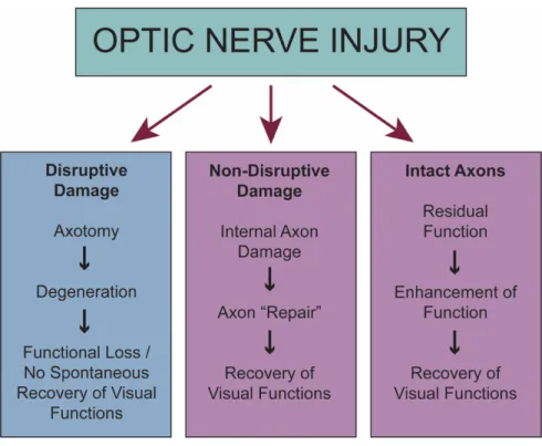
Figure 7. Possible axonal outcomes following injury to the optic nerve.

Following an optic nerve injury, there are three outcome possibilities: a tearing or severe damage to the axon resulting in axotomy (left), internal damage but some axonal function was retained (middle), or the axon remained relatively intact (right) (figure adapted from Sabel, 1999).

4.1. Behavioural Evaluation of Recovery

In general, researchers have studied the loss of neurons by evaluating changes in morphology, imaging, electrophysiology, and behaviour (Yoles & Schwartz, 1998). To evaluate

(28)

plasticity in relation to the loss of neurons, studies will often turn to behavioural measures of recovery. For example, in studies on visual recovery, VA is often a measure used to determine if visual performance has changed. There are many ways to measure visual thresholds of acuity and contrast sensitivity in rodents (see Huberman & Niell, 2011 for review). One of the simplest ways to test vision in mice is the visual placing test. Essentially, the mouse is held by the tail 15 cm above a grid. The mouse is then lowered in a decelerating fashion towards the grid until the mouse extends its paws (Leinonen & Tanila, 2017). This test measures the mouse’s perception of depth and visual acuity, i.e. as the grid approaches the mouse’s face, there is a change in depth and the grid’s spatial resolution appears larger. However, this method does not allow for much quantification as the distance at which the mouse believes it can reach out and grasp the grid is only an approximation of visual ability and does not measure the exact visual acuity or depth perception threshold. A method of measuring specific VA is to test their optomotor or optokinetic response. This involves an apparatus that presents drifting sinusoidal gratings, which the rodent will automatically track the movement with a head (optomotor) or eye (optokinetic) movement (Prusky, Alam, Beekman, & Douglas, 2004). The spatial frequency of the gratings is then gradually increased until the tracking movement is no longer observed, i.e. the animal’s visual acuity threshold has been reached and it can no longer detects the gratings. However, these reflexes mostly involve subcortical areas via the SC and AOS (Huberman & Niell, 2011). In order to measure more complex visual tasks, reinforcement-based discrimination tasks such as the water maze discrimination task are often used, in which the rodent is trained to swim towards two screens separated by a small divider. The rodent must swim towards the screen presenting a grating in order to reach the platform and get out of the water. The grating is increased in spatial frequency until the rodent is no longer able to discriminate (Prusky et al., 2000). However, water maze tasks require a training session of 1 week or more and the mouse is stressed by being submerged in water as mice are not good swimmers. For other visual functions, the visual cliff test is a useful option for testing depth perception and behavioural responses based on visual cues. Naturally, a mouse will fear falling as it could lead to injury. Therefore, by simulating a cliff using visual cues, a mouse will elicit avoidance behaviours and refrain from going “over the cliff” if it can discriminate the change in depth (Seabrook et al.,

(29)

2017). There are various approaches to the test methodology and measurement, but the purpose remains the same (e.g. de Lima et al., 2012; Lim et al., 2016).

5. Objectives and Rationale

In this thesis, we explore the hypothesis that spontaneous recovery of visual functions is possible at the behavioural level following an optic nerve injury in mice, and that recovery is dependent on the survival of residual RGCs. This thesis will combine optic nerve injury models of varying severities with modern visual behaviour analyses to evaluate various pathways of the visual system. The optic nerve injury models of varying severities have previously been implemented in rats, but never in mice. This approach opens up a new facet of research examining the recovery of visual functions in mice while varying the extent of the optic nerve damage. The investigation of these functions is of primary interest given the growing use of wild-type and genetically modified mice in vision and neuroscience. To evaluate the recovery of visual functions in our model, the optomotor reflex test and the visual cliff test were chosen as they involve various specific structures in the visual system. The optomotor reflex test involves subcortical processing via the SC and AOS, while the visual cliff test involves conscious perception of visual cues and exploration via the primary visual pathway. Both tests are easily implemented with less training and avoid confounding variables such as learning or motor skills (e.g. the water maze). Additionally, the association between surviving RGC distribution and recovery of visual functions following a pONC has never been examined in the mouse model. Therefore, the specific objectives addressed in this thesis are 1) to measure the spontaneous recovery of visual functions following two pONC severities using two behavioural tests and 2) to determine the percentage and distribution of retinal ganglion cell survival following an optic nerve injury.

(30)

Methods

1. Animal Preparation

All procedures were accepted by the Comité de déontologie de l’expérimentation sur les animaux (CDEA) de l’Université de Montréal (CDEA 17-010) and were in accordance with the guidelines of the Canadian Council for the Protection of Animals (CCPA). In the present study, 14 C57BL/6 male adult mice (Charles River Laboratories, Inc., Senneville, QC, Canada) were used, separated into two groups (n = 7 each). One group of mice received a bilateral high intensity pONC, while the other group received a bilateral low intensity pONC. The animals were maintained in a 12h light/dark normal daylight cycle and had access to food and water ad

libidum.

2. Visual Deficit

A pONC was induced bilaterally to create a diffuse loss of vision. First, mice were anesthetized with a constant flow of isoflurane gas (O2 dispensed at 1L/min, isoflurane 3%) by

inhalation. While under a microscope, a small incision was made in the temporal inferior quarter of the conjunctiva. Then, using self-closing calibrated cross-action forceps (Fig. 8), the incision was widened until the optic nerve was exposed. The optic nerve was pinched with the calibrated forceps, either fully (high-intensity pONC) or with a pre-measured space of 0.152 mm (low intensity pONC). The optic nerve was pinched for 3 seconds, approximately 2 mm from the back of the eye. An antibiotic gel, Ciloxan® (Alcon, Fort Worth, TX, USA) was then topically applied to the surgical area to prevent infection, and the animal was monitored following surgery.

(31)

Figure 8. Forceps used to perform a partial optic nerve crush.

These calibrated cross-action forceps produce a pONC with a pre-defined intensity by altering the space left between the forceps at closed position. In this case, no space was calibrated for the high intensity pONC, and a space of 0.152mm at closed-position was used for the low intensity pONC.

3. Assessment of Visual Functions

Two behavioural tests were used to evaluate baseline visual functions and recovery over time following a pONC (Fig. 9). Specifically, the optomotor reflex test was performed on days 1, 3, 7, 14, 21, and 28 post-pONC, while the visual cliff test was performed on days 1, 14, and 28 post-pONC. After 4 weeks post-pONC, the mice were sacrificed, and the retinas were dissected. Then, a 7-day immunofluorescence technique was used to quantify RGCs.

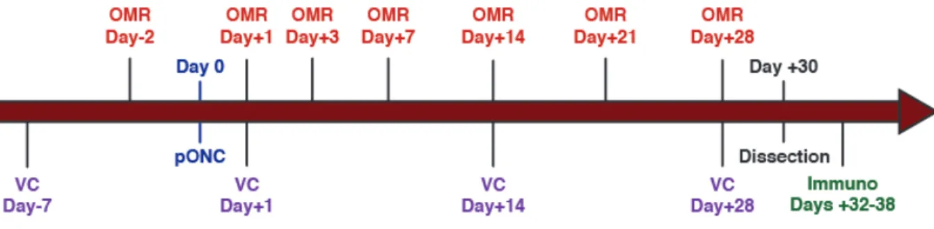
Figure 9. Timeline of experiments.

Two visual behaviour tests were completed once prior to injury, then at various time points for up to 28 days. Mice were then sacrificed, retinas were dissected, and immunofluorescence was completed for cell quantification. OMR = Optomotor Reflex test; VC = Visual Cliff test; pONC = partial Optic Nerve Crush; Immuno = Immunofluorescence.

(32)

3.1. Optomotor Reflex

The optomotor reflex was tested using behavioural procedures via the OptoMotryTM_{apparatus (Cerebral Mechanics, Inc., Lethbridge, AB, Canada). The apparatus}

consists of four computer screens, forming a 360-degree visual stimulation (Fig. 10). A camera in the apparatus relays a live transmission to the OptoMotryTM_{HD 2.0.0 software on a separate}

computer which allows for manipulation of the stimuli and observation of the animal’s behaviour. First, the mice were habituated to the apparatus over the course of three days (5, 10, 15 minutes), alternating grey screen and moving vertical sinusoidal gratings (0.050 cpd). The apparatus was cleaned with water following each test. Once the habituation was complete, the mice were tested prior to the pONC, then 1, 3, 7, 14, 21, and 28 days following the deficit. During testing, each mouse was placed in the apparatus and was presented with 0.050 cpd vertical sinusoidal gratings for 3 seconds. Mice were observed during the grating presentation; if the animal followed the movement of the grating with its head, then the spatial frequency was considered to have been detected. Full contrast spatial frequencies moving in both clockwise and counter clockwise directions (allowing for the assessment of the right and left eye’s VA, respectively) at a speed of 12.0 d/s were increased in an adaptive staircase order (from 0.050 cpd to 0.550 cpd) until no reflex was observed.

(33)

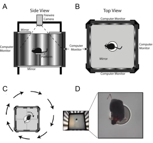
Figure 10. Optomotor reflex test.

A and B. Side and top view representations of the OptoMotryTM_{apparatus. The mouse is placed on a raised platform}

surrounded by computer monitors presenting moving sinusoidal gratings. C. As the gratings move in one direction or the other, the mouse will track the grating with a head movement in the same direction (figures obtained from Prusky et al., 2004). D. Image of a mouse during an optomotor response. The red star indicates that the grating rotation is centered on the mouse’s head position.

3.2. Visual Cliff

The visual cliff test is designed to assess functional vision by relying on an animal’s ability to discriminate changes in depth, based solely on visual cues. Specifically, animals will naturally avoid a change in depth drastic enough to result in a fall. In this study, a plexiglass box (40 cm L x 10 cm W x 20 cm H) was positioned on a table so that half of the box was positioned directly over a 60 cm2_{, 2 cm x 2 cm checkboard pattern (“shallow end”), while the other half}

(34)

was suspended 70 cm above the same checkerboard pattern (“deep end”) (Fig. 11). This setup does not change or vary between tests. For each test, the mouse was placed in the back of the “shallow end” and movements were recorded for two minutes. The total time in the “shallow end” was noted, and the box was cleaned with water between each assessment. This test was performed once prior to the pONC, then 1, 14, and 28 days following the deficit. To measure visual loss and recovery, a “Shallow End Index” was calculated as follows:

"Shallow End" Index = TDE-TSE T_TOTAL

TDE is the total time spent in the “deep end”, TSE is the total time spent in the “shallow end”,

and TTOTAL is the total time of the test (in this case, 2 minutes). Therefore, a positive index value

indicates that more time was spent in the “shallow end”. As the values approach 0, the difference between time spent on each end decreases, suggesting that the mouse no longer discriminates the change in depth illusion.

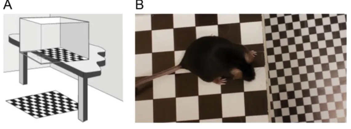
Figure 11. Visual cliff test.

A. Schematic representation of the visual cliff apparatus (figure obtained from Glynn, Bortnick, & Morton, 2003). B. Image of mouse exhibiting avoidance behaviour by hesitating at the line between “shallow end” and “deep end”.

(35)

4. Retinal Ganglion Cell Quantification

After day 28, mice were deeply anesthetized with 10% urethane (2 g/kg, i.p.) and perfused transcardially with 4% paraformaldehyde in 0.1 M phosphate buffer solution (PBS) at room temperature. Eyes were dissected from the specimen and two small holes were pierced in the cornea. The eyes were post-fixated in 4% paraformaldehyde in 0.1 M PBS overnight. The retina was then dissected under microscope from the globe, and four incisions were made to allow for flat-mounting. Flat-mounted whole retinas were pre-incubated overnight at 4°C in 0.1 M PBS with 0.5% triton, 10% goat serum, and 1% bovine serum albumin (BSA). Retinas were then immunostained with a rabbit polyclonal anti-RNA-binding protein with multiple splicing (anti-RBPMS) antibody (1:500; PhosphoSolutions, Aurora, CO, USA) in 0.1 M PBS-triton-0.5%, 3% goat serum, and 1% BSA for 48 hours at 4°C, followed by Alexa Fluor 488 goat anti-rabbit IgG antibody (1:500, Cedarlane, Burlington, ON, Canada). Finally, retinas were incubated for 1 hour in Hoescht 33258 solution (1:10 000; Sigma-Aldrich, Co., St. Louis, MO, USA) in 0.1M PBS. Retinas were mounted onto gelatinous slides with FluoroshieldTM_histology

mounting medium (Sigma-Aldrich, Co., St. Louis, MO, USA), and a coverslip was placed. RGCs were imaged under fluorescence microscopy (100x) using the Leica DMRB microscope (Leica Microsystems, Wetzlar, Germany) with QImaging Colour Camera (Teledyne QImaging, Surrey, BC, Canada), an FITC filter (Chroma Technology Corp., Bellows Falls, VT, USA), and Stereo Investigator®_{software (version 11; MBF Bioscience, Williston, VT, USA). Images were}

increased to 400x magnification and adjusted in Adobe Photoshop CC software (version 20.0.3, Adobe Inc., San Jose, CA, USA). RGCs were quantified manually in 8 pre-determined 1 mm2

areas: 4 proximal and 4 distal areas to the optic disk.

5. Statistical Analysis

All statistical analyses were performed with SPSS software (version 25; IBM Corp., Armonk, NY, USA). Due to the nature of the data and sample size, all analyses were non-parametric. The optomotor reflex data were analyzed using a Friedman test for within-subject repeated measures with a significance level of p < 0.05, to evaluate whether a recovery

(36)

developed over time following the pONC (days 1-28). Wilcoxon signed rank tests were used to evaluate VA loss by comparing the pre-ONC data to day 1. If the Friedman test was significant, Wilcoxon signed rank tests were also used to compare days 3, 7, 14, 21, and 28 to day 1, thus determining at what time significant recovery began. Visual cliff test data (“Shallow End Index”) were similarly analyzed using a Friedman test with a significance level of p < 0.05, to evaluate whether a recovery developed over time following the pONC (days 1-28). Wilcoxon signed rank tests were used to evaluate loss of depth perception by comparing the pre-ONC data to day 1. If the Friedman test was significant, Wilcoxon signed rank tests were also used to compare days 7, 14, and 28 to day 1, thus determining at what time significant recovery began. Mann-Whitney U tests with a significance level of p < 0.05 were used for RGC quantification data, to compare the cell loss following a high or low intensity pONC against control retinas. Mann-Whitney U tests were also used to compare proximal and distal region cell counts for the two intensities and control retinas.

(37)

Results

1. Optomotor Reflex

The high-intensity pONC resulted in a total loss of vision in both the right (Wilcoxon, p = 0.008) and left (Wilcoxon, p = 0.008) eyes, with no visual recovery in the following 28 days (Fig. 12A). The low intensity pONC also resulted in a significant loss of vision in both the right (Wilcoxon, p = 0.008) and left (Wilcoxon, p = 0.008) eyes. However, a significant recovery of visual function was observed over time (Friedman, right eye, c2_{= 38.045, p = 0.000; left eye,}

c2_{= 36.242, p = 0.000), starting at day 3 (Wilcoxon, right and left eyes, p = 0.008) and remaining}

(38)

Figure 12. Changes in visual acuity over time, as measured by the optomotor reflex test.

A. Acuity pre- and post-high-intensity pONC. Note the sudden decrease in acuity, and no recovery in the following 28 days. B. Acuity pre- and post-low intensity pONC. There is a sudden decrease in acuity, then a 39% recovery in the left eye, and 57% recovery in the right eye.

2. Visual Cliff

During the visual cliff test, the high-intensity pONC group initially spent significantly more time in the “shallow end” before injury (Wilcoxon, p = 0.018), exhibiting hesitant behaviours and avoiding the deep end on the apparatus. The preference for the “shallow end”

(39)

did not return in the following 28 days (Friedman, c2_{= 1.143, p = 0.565) (Fig. 13A). As with}

the high-intensity pONC mice, the low intensity bilateral pONC mice showed a loss of preference for the shallow end after the injury (Wilcoxon, p = 0.018). However, a significant recovery of visual function was observed over time (Friedman, c2_{= 6.000, p = 0.050), which}

mainly occurred between day 14 and day 28 (Wilcoxon, p = 0.018) (Fig. 13B).

Figure 13. Changes in depth perception over time, as measured by the visual cliff test.

A. “Shallow End Index” pre- and post-high-intensity pONC. Notice the decrease in time spent in the “shallow end” suggesting that the mouse cannot discriminate the change in visual cues. This discrimination does not return in the following 28 days. B. “Shallow End Index” pre- and post-low intensity pONC. Preference for the “shallow end” is no longer observed at day 1 post-pONC, but preference returns fully by day 28 post-pONC.

(40)

3. Retinal Ganglion Cell Quantification

In control mice, the average RGC count in one 1 mm2_{quadrant was 772 cells. There was}

no significant difference between proximal and distal cell regions (Mann-Whitney, p = 0.086) (Fig. 14A). Following the bilateral high intensity pONC, the RGC survival was about 16.8%. However, there was a significant difference between proximal and distal distribution (Mann-Whitney, p = 0.008) with less surviving cells in the proximal regions than distal regions. The bilateral low intensity pONC resulted in a higher percentage of surviving RGCs at 67.0%, with no significant difference between regions (Mann-Whitney, p = 0.127). There was a significant difference in cell count between control and high intensity pONC retinas (Mann-Whitney, p = 0.000), between control and low intensity pONC retinas (Mann-Whitney, p = 0.000), and between high and low intensity pONC retinas (Mann-Whitney, p = 0.000) (Fig. 14B).

(41)

Figure 14. Retinal ganglion cell quantification.

A. Comparisons between proximal and distal cell quadrants for control, high intensity, and low intensity pONC retinas. B. Comparison between control, high intensity, and low intensity pONC total cell quantification. Note the higher cell survival rate following the low intensity pONC compared to the high intensity pONC.

(42)

Discussion

The research addressed in this thesis aimed to determine whether visual functions could recover spontaneously following two pONC severities. This was measured using two behavioural tests: the optomotor reflex test and the visual cliff test. By measuring recovery with these two tests, changes in visual functions could be observed during subcortical and cortical processing, respectively. RGC loss was also quantified to determine whether recovery of visual functions was dependent on residual cell survival. The data presented in this thesis has demonstrated that behavioural recovery of visual functions is dependent on the proportion of surviving cells, and therefore the severity of the optic nerve injury.

1. Interpretation of Results

With both high and low intensity pONCs, there was a sudden loss of visual functions after injury, as measured by the optomotor reflex and visual cliff tests. Following the high intensity pONC, no recovery of visual functions occurred in the following 28 days, as measured by the optomotor reflex and visual cliff tests. This is consistent with previous studies using a similar high intensity pONC method (de Lima et al., 2012). As the intensity of this injury should not allow for survival of many intact axons, it is not surprising that no recovery occurred at the behavioural level. The behavioural results also reflect the difference in RGC survival rate. The high intensity pONC resulted in only 16.8% RGC survival, suggesting that not enough retinal input was able to be processed cortically or subcortically for a behavioural response to be elicited. This percentage is consistent with other studies using a very similar pONC technique, in which there was a 27% RGC survival after 2 weeks and an 8% survival after 8 weeks (Levkovitch-Verbin, 2004; Levkovitch-Verbin et al., 2000). However, other studies in rats have shown that recovery can be possible with as low as 10% RGC survival using a simple brightness detection test (Sabel, 1999). Therefore, the nature of the task could determine the amount of visual input required for recovery of the particular visual function involved. The visual input threshold may also vary between species due to biological or behavioural differences. Surprisingly, there was also a difference between proximal and distal region cell counts. There

(43)

are multiple reasons as to why this could occur, one being that there could have been more fluorescence background in the retinal images, making the quantification more difficult in proximal regions. This was minimized as much as possible by thoroughly removing the vitreous humour. Differences in RGC survival between proximal and distal regions could also be due to the force applied by the forceps. One of the few limitations of the pONC procedure is the inability to measure the exact amount and distribution of the force applied to the optic nerve (Levkovitch-Verbin, 2004).

Following the low intensity pONC, some recovery of VA was observed with the optomotor reflex test as early as day 3 post-pONC, showing that the severity of injury does indeed have an effect on recovery potential. With the visual cliff test, the mice demonstrated clear avoidance behaviors toward the “deep end”, opting to spend about ¾ of the time in the “shallow end”. This preference was lost after injury, but then the preference and behaviors returned significantly by day 28 post-pONC. This difference between injury severities was illustrated in the study on rats by Rousseau and Sabel (2001), who demonstrated that recovery can occur with a mild pONC (i.e. leaving a calibrated space of 0.2 mm between forceps at closed position), but not with a moderate pONC (calibrated space of 0.1 mm) or severe pONC (no calibrated space). This study was completed with a 6-choice contrast discrimination task, therefore differing in the method used to evaluate changes in vision. Previous studies on spontaneous recovery also exhibited similar timelines, showing a maximum recovery around 2-3 weeks post-injury (Sabel, 1999) compared to the maximum recovery at 2-3-4 weeks in the present study. The low intensity pONC resulted in a survival rate of 67.0% due to the reduced force involved in the mechanism of injury (i.e. the forceps were not closed completely), which is consistent with observed improvements in visual functions. The lack of difference in survival percentage between proximal and distal regions supports previous studies showing a lack of retinotopic organization in the optic nerve. There was also a difference in the recovery of VA in the right versus left eye. The right eye showed about 18% more recovery than the left eye. This could be due to experimenter bias, as a pONC is more difficult on the left eye when the experimenter is left handed. Another explanation for this discrepancy could be ocular dominance, in which the visual input from one eye is favoured more than the other. Approximately two thirds of the human population are innately right eye dominant

(44)

(Momeni-Moghaddam, McAlinden, Azimi, Sobhani, & Skiadaresi, 2014). Though this lateralization has been observed in some other species such as monkeys (Porac & Coren, 1976), it is unclear whether mice have an innate dominant eye.

As summarized by the injury outcomes proposed by Sabel (1999), some axons will only suffer minor damages and retain abilities following a pONC. This non-disruptive damage still allows for the “repair” of damaged axons over time via endogenous processes. Other RGCs will remain relatively intact with unaffected functions. These two injury outcomes allow for plasticity and reorganization of visual input to the CNS. Specifically, the signals from residual cells would become more salient in visual processing and would be relied on for visual behaviour. In order for this reorganization to occur, there must be a certain amount of minimal residual structure in order for visual recovery to occur spontaneously. As no recovery was observed at the behavioural level following an RGC survival rate of 16.8%, it can be deduced that a certain percentage of cell survival must remain after the injury in order to recover visual functions. As some studies have reported a recovery of vision with as low as 10% residual cells in rats (Sabel, 1999) or higher at 70% residual cells in goldfish, it is possible that the threshold varies between species and is task-dependent. Specifically, certain visual tasks may require more visual input to recover than others.

2. Justification of Methods

C57BL/6 male adult mice were used in the present study as they are a widely used strain of mice in sensorineural research. They are easy to breed, have a relatively good lifespan (at least two years), and have a lower susceptibility to tumours than many other mouse strains. C57BL/6 mice are also excellent for expressing mutations, making them an asset for transgenic model creation. As male rodents perform spatial tasks better than females (e.g. Morris water maze), specifically in object localization and recognition (Frick & Gresack, 2003), only males were used in this study.

The bilateral pONC is an extensively used model of diffuse axonal injury in rodents (Levkovitch-Verbin, 2004; Prilloff, Henrich-Noack, Kropf, & Sabel, 2010; Sabel, 1999). This

(45)

model of injury is ideal for studying the underlying mechanisms of the visual system, as well as plasticity and recovery of visual functions. With the pONC, the severity of injury can also be controlled in order to mimic various stages of degeneration and/or damage and will reflect injuries or diseases that leave some residual cells. In this study, the intensity of the pONC was determined based on the size of the optic nerve. As the mouse has an optic nerve diameter of about 0.3-0.4 mm (Honjin, Sakato, & Yamashita, 1977), we wanted to have one pONC intensity that would have a maximum possible impact (high intensity), and another that would, hypothetically, leave about half the nerve relatively intact (low intensity). In this case, a 0.152 mm space would preserve about half of a 0.3 mm optic nerve. A bilateral approach was used in this case due to the nature of the behavioural tests (e.g. the visual cliff would be ineffective if one eye can still detect visual cues). The duration of the pONC (3 seconds) was determined based on previous publications on the pONC in murine models (Puyang et al., 2016; Tang et al., 2011), and a temporal orbital approach was used as it is less invasive and time consuming (Levkovitch-Verbin, 2004).

The two behavioural tests used in this study were chosen based on the visual pathways involved. The optomotor reflex test provided a quick test of VA with very little training. This is remarkably convenient, as other VA tests (e.g. visual water test) often require lengthy training sessions and some sort of positive or negative reinforcement. These tests also require some learning and motor skills, and therefore could be affected by non-visual performance factors (Leinonen & Tanila, 2017; Prusky et al., 2000). Another advantage of the optomotor reflex test is its ability to measure monocular responses. By making the gratings drift clock-wise, the left eye acuity can be measured due to the lateral position of the eyes in mice. Identically, by making the gratings drift counter-clock-wise, the right eye acuity can be measured. In addition, the optomotor reflex is a subcortical response, allowing researchers to observe subcortical function. The visual cliff test takes advantage of the animal’s innate fear of falling by using visual cues. This test, as it involves exploratory behaviour based on visual cues of depth, is substantially processed by the primary visual pathway as it involves dLGN processing and functional binocular vision (Leamey et al., 2007). One of the primary advantages of this test is that it is quick and easy to perform. The test is also easily adapted for assessing various species, and is notably used to assess human infants (Leinonen & Tanila, 2017). The visual cliff test was

(46)

performed less often than the optomotor reflex test to avoid any impact of memory on test performance.

To determine cellular changes, immunofluorescence techniques can be used to analyze the presence of surviving cells. The technique used in this study consisted of targeting a specific cell-type with a primary antibody that binds to a molecule (e.g. protein, enzyme, etc.). Then, a secondary fluorophore-conjugated antibody binds to the primary antibody and emit at a particular wavelength. This indirect (secondary) technique offers greater sensitivity than direct immunofluorescence because more than one secondary antibody can bind to a single primary antibody, which results in an amplification of signal emission. The marker used in this study, an RBPMS antibody, targets the somas of the entire RGC population. This marker can target all RGC-types, is only localized in RGCs, and distributes fairly evenly in the cell soma (Rodriguez, de Sevilla Muller, & Brecha, 2014), making it an ideal marker for RGC survival. This marker can also be used on a wide variety of models other than mice, including guinea pigs, rabbits, rats, and macaque monkeys. The selective marker has even been specifically used to observe RGCs after a pONC in recent studies (Rodriguez et al., 2014). Other specific markers for RGCs include the Brain-specific hemeobox/POU domain protein 3A (Brn3a), however it has been shown to only identify about 85% of the mouse RGC population, and TRPV4, but it lacks specificity as it also targets Müller cells (Zalis, Johansson, & Englund-Johansson, 2017). Therefore, the RBPMS antibody provides the most selective RGC marking.

3. Future Directions and Clinical Implications

Given the results of the present thesis, it appears that visual functions can only be measured behaviourally if there are enough surviving cells to send signals through the various visual pathways. Evidently, this poses the question of how many RGCs need to survive in order to see a recovery of visual functions. Based on the RGC survival rates following the high and low intensity pONCs, the threshold of RGC survival lies somewhere between 16.8% and 67.0%. The next step would therefore be to conduct the same research procedures using multiple calibrated pONC intensities between no space and the 0.152 mm2_{space at closed position. As}