Approximate Loop Unrolling

HAL Id: hal-01401828

https://hal.inria.fr/hal-01401828

Preprint submitted on 23 Nov 2016

HAL is a multi-disciplinary open access

archive for the deposit and dissemination of

sci-entific research documents, whether they are

pub-lished or not. The documents may come from

teaching and research institutions in France or

abroad, or from public or private research centers.

L’archive ouverte pluridisciplinaire HAL, est

destinée au dépôt et à la diffusion de documents

scientifiques de niveau recherche, publiés ou non,

émanant des établissements d’enseignement et de

recherche français ou étrangers, des laboratoires

publics ou privés.

Approximate Loop Unrolling

Marcelino Rodriguez-Cancio, Benoit Combemale, Benoit Baudry

To cite this version:

Marcelino Rodriguez-Cancio, Benoit Combemale, Benoit Baudry. Approximate Loop Unrolling. 2016.

�hal-01401828�

Approximate Loop Unrolling

Marcelino

Rodriguez-Cancio

[email protected]

Benoit Combemale

[email protected]

Benoit Baudry

[email protected]

ABSTRACT

We introduce Approximate Unrolling, a loop optimiza-tion that reduces execuoptimiza-tion time and energy consumpoptimiza-tion, exploiting the existence of code regions that can endure some degree of approximation while still producing acceptable sults. This work focuses on a specific kind of forgiving re-gion: counted loops that map a given functions over the elements of an array. Approximate Unrolling transforms loops in a similar way Loop Unrolling does. However, un-like its exact counterpart, our optimization does not unroll loops by adding exact copies of the loop’s body. Instead, it adds interpolations.

We describe our experimental implementation of Approx-imate Unrolling in the Server (C2) Compiler of the Open-JDK Hotspot JVM. The choice to implement our technique directly in the compiler reduced Phase Order problems and transformation overhead. It also proved that our technique could actually improve the performance of a production-ready compiler. Using our modified version of the com-piler, we perform several experiments showing that Ap-proximate Unrolling is able reduce execution time and energy consumption of the generated code by a factor of 50% with minimal accuracy losses.

Keywords

approximate computing; compiler optimizations; loop un-rolling

1.

INTRODUCTION

Approximate computing exploits the fact that some com-putations can be made less precise and still produce good results in order to reduce execution times and energy con-sumption [25]. Previous works in the field have proven that when small reductions in accuracy are acceptable, significant improvements in execution times and energy consumption can be achieved [41]. Opportunities for approximation arise all along the stack and researchers have proposed techniques to approximate in both hardware and software.

Permission to make digital or hard copies of all or part of this work for personal or classroom use is granted without fee provided that copies are not made or distributed for profit or commercial advantage and that copies bear this notice and the full citation on the first page. To copy otherwise, to republish, to post on servers or to redistribute to lists, requires prior specific permission and/or a fee.

Copyright 2014 ACM X-XXXXX-XX-X/XX/XX ...$15.00.

Hardware-oriented approximation techniques have proposed components with approximation capabilities, such as FPUs [38], adders [16, 33] and memories [10, 20]. They also ex-ploit the inherent non-determinism of existing hardware as sensors [21] and wireless adapters [32] and some even ex-pose it to developers [7, 36]. On the software-oriented side of approximate computing, the proposed techniques mod-ify existing algorithms automatically [34, 24, 28] or provides support for programming with approximation via language design [23, 30], frameworks [6, 7] and compilers [4].

In this work we describe a loop optimization, namely Ap-proximate Unrolling, that uses the ideas of apAp-proximate computing to reduce execution times and energy consump-tion of loops mapping values to arrays. These loops are commonly encountered in programs that process signals and that exploit heuristics. In addition, these loops account for a large part of the computation, e.g., the loops that we an-alyze in our case study are executed millions of times in a few seconds. Consequently, saving resources on these loops can have a major impact on the program’s consumption, as long as the results remain acceptable for the users.

The key insight of Approximate Unrolling relies on the following observation: data such as time series, sound, video and 3D Meshes are frequently represented as arrays where contiguous slots contain similar values. As conse-quence of this neighboring similarity, computations produc-ing this data are usually locally smooth functions. In other words, computations producing or modifying nearby array values representing these kinds of data frequently yield sim-ilar results.

Our technique exploits this observation by searching for loops where computations results are assigned to contiguous array slots in each iteration. Then, we substitute some of these computations by inexpensive interpolations of the val-ues assigned to nearby array valval-ues. In exchange for this loss in accuracy, we obtain a faster and less energy consuming loop.

To substitute iterations, Approximate Unrolling works in a similar way as Loop Unrolling. Yet, instead of un-rolling by adding exact copies of the loop’s body, it adds code that interpolates the computations performed by the original loop, creating approximate iterations that interpo-late some mappings. The code of the approximate iteration is minimal, thus reducing execution time and energy con-sumption of the whole loop.

We have modified the OpenJDK Java Server (C2) com-piler to include Approximate Unrolling as a machine-independent optimization. All machine-machine-independent

opti-mizations (and therefore ours as well) reshape the C2’s in-ternal representation of a program to obtain an optimized version of the same program. Approximate Unrolling performs an static analysis over the C2’s Internal Represen-tation (IR) to find loops matching certain pattern. Then, those loops are transformed by reshaping the C2’s IR.

Our initial implementation of Approximate Unrolling relied on source code and bytecode transformations. Unfor-tunately this led to a phase ordering problem, breaking other compiler optimizations and failing to gain the expected per-formance. We then decided to implement the optimization directly in the compiler, allowing us to respect the existing phase order. This also reduced the overhead since we had a direct access to the internal representations provided by the compiler. In addition, this gives us garantees about the fact that Approximate Unrolling can actually has an impact on the performance of a highly optimized code created by production-ready compiler.

Our experiments shows that Approximate Unrolling is able to reduce the execution time and energy consumption of the x86 code generated around 50% to 80% while reducing the accuracy to acceptable levels.

The contributions of this work are:

• Approximate Unrolling, an approximate loop trans-formation

• A formal specification of loops targeted by Approxi-mate Unrolling and of the behavior of the transfor-mation

• An efficient implementation of Approximate Un-rolling inside the OpenJDK Hostpot VM.

• An empirical assessment of the effectiveness of Ap-proximate Unrolling to trade accuracy for time and energy savings.

The rest of the paper is organized as follows, in section 2 we describe our optimization and its scope. We then detail our implementation in section 3 and our evaluation in sec-tion 4. Secsec-tion 6 describes how Approximate Unrolling compares with other approximate computing techniques and finally section 7 concludes.

2.

APPROXIMATE UNROLLING

In this section we describe the main contribution of our paper, which is the Approximate Unrolling approximate loop optimization. We first introduce the intuition of the optimization using the toy example of listing 1. Afterwards, we formally characterize the loops that Approximate Un-rolling can target. Finally, we introduce the formal seman-tics governing the proposed optimization.

2.1

Illustrating Example

Approximate Unrolling creates an alternative version of the loop by unrolling it with operations that interpolate the computations performed in the loop’s original body. We propose two variants: linear or nearest neighbor interpola-tions. Both are supported by our implementation, which is able to choose one single transformation for each loop.

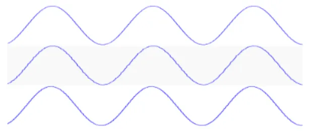
The loop of listing 1 will serve to illustrate both trans-formations. The loop maps a sine wave into an array and belongs to a music synthesizer. Conceptually, the example

loop transformed by Approximate Unrolling using linear interpolation looks like the one in listing 2, while the same loop approximated with nearest neighbor looks like the one in listing 3. The output of these loops is depicted in figure 1.

@ A p p r o x i m a t e double A [] = new double [ N ]; double stride = Math . PI * 2 / N ;

f o r ( i n t i = 0; i < N ; i ++ ) A [ i ] = M ath . sin ( i * s t r i d e ) ;

Listing 1: A loop mapping a sine wave into an array double A [] = new double [ N ];

double stride = Math . PI * 2 / N ; A [0] = M ath . sin (0) ; f o r ( i n t i = 2; i < N ; i += 2 ) { A [ i ] = M ath . sin ( i * s t r i d e ) ; A [ i - 1] = ( A [ i ] + A [ i - 2]) * 0.5 f ; } i f ( i == N ) A [i -1] = Math . sin (( i - 1) * s t r i d e ) ;

Listing 2: The loop of listing 1, transformed by Approximate Unrolling using linear interpolation double A [] = new double [ N ];

double stride = Math . PI * 2 / N ; f o r ( i n t i = 0; i < N ; i += 2 ) {

A [ i ] = M ath . sin ( i * s t r i d e ) ; A [ i + 1] = A [ i ]; }

Listing 3: The loop of listing 1, transformed using nearest neighborg interpolation

Figure 1: Sine waves generated by the motivation examples. The upper wave is generated by the loop of listing 1, while the middle and lower ones are generated by loops of listing 2 and 3, respectively.

As the modified loop of listing 2 shows, when using linear interpolation, Approximate Unrolling adds code to the loop’s body that interpolates the computations of the odd iterations as the mean of the even ones(the computations of iteration one are interpolated using the results of iterations zero and two, computations of iteration three are interpo-lated using the results of two and four and so on). Initially, Approximate Unrolling peels iteration zero of the loop. Then, it modifies the initialization and updates the state-ments to double the increment of the loop’s counter variable. As result of this, if the original loop performed an even num-ber of iterations, the last iteration would not be performed. To cover for this case, Approximate Unrolling also peels the last iteration.

The procedure with nearest neighbor is quite similar, Ap-proximate Unrolling only modifies the update statement to double the increment of the loop’s counter variable. It also adds code with the nearest neighbor interpolation at the end of the loop’s body.

i, n ∈ Z B ∈ {expression} [[B]] ∈ {true, f alse} t body = C I0, C ⊂ {statement} ξ = hB, i := i + n, Ci

Figure 2: Common definitions and rules used by both linear and nearest neighbor transformations

ForL

(F orL(I0, B, i := i + n) C, σ) → (I0; if (B) P re(ξ) else SKIP, σ)

ExL

(ExL(ξ), σ) → (i := i + 2 ∗ n; if (B) C; AprxL(ξ) else P ost(ξ), C, σ)

AprxL

(AprxL(ξ), σ) → (a[i − n] := (a[i] + a[i − 2 ∗ n]) ∗ 0.5; ExL(ξ), σ)

Pre

(P re(ξ), σ) → (C; ExtL(ξ), σ)

Post

(P ost(ξ), σ) → (i := i − n; if (B) C; i := i + n; else SKIP, σ)

Figure 3: Small step SOS of Approximate Unrolling using linear interpolation

ForN

(F orN(I0, B, i := i + n) C, σ) → (I0; ExN(ξ), σ)

ExN

(ExN(ξ), σ) → (if (B) C; AprxN(ξ), else SKIP, σ)

AprxN

(AprxN(ξ), C, σ) → (i := i + n; if (B)a[i] := a[i − 1]; i := i + n; ExN(ξ) else SKIP, σ)

Figure 4: Small step SOS of Approximate Unrolling using nearest neighbor

htarget for i ::= ‘for’ ‘(’ hexpressioni ‘;’ hexpressioni ‘;’ hupdate expressioni ‘)’ ht bodyi

hupdate expr i ::= hidentifier i ‘+=’ hinteger i

ht bodyi ::= ‘{’ hstatementi harray assigni hstatementi ‘}’

harray assigni ::= hexpressioni ‘[’ hindex expr i ‘]’ ‘=’ hexpressioni

hindex expr i := hexpressioni

Grammar 1: Grammar of for loops targeted by Ap-proximate Unrolling

2.2

Target Loops

Our optimization targets the subset of Java for loops that (i) have an update expression that increments or decrements a variable by a constant value (ii) contain an array assign-ment inside its body (iii) the indexing expression of the array assignment is value-dependent on the loop’s update expres-sion.

We now use Backus-Naur form to formalize the syntax of the loops abiding to (i) and (ii), while (iii) is formalized using data flow equations. For the sake of simplicity, we only show the case in which the variable is being incremented. It should not be difficult for the reader to derivate these rules for the case in which the variable is being decremented.

Grammar 1 shows the BNF rules defining the kind of loops Approximate Unrolling can target. In the grammar, the non-terminal rules hexpressioni, hidentif ieri, hintegeri and hstatementi, define the Java expressions, identifiers,

inte-ger literals and statements respectively. Rule htarget f ori describes the loops targeted by Approximate Unrolling. The rule introduces two other terminals. The first non-terminal: hupdate expri describes the expected update ex-pression or the loop, consisting in a variable being incre-mented by a literal value, while ht bodyi describes a list of statements containing at least one array assignment, which are described using the harray assigni non-terminal.

The hindex expri rule reduces to a Java expression and facilitates the formalization of condition (iii), which we do as follow: let L be a loop conforming to Grammar 1, let AL

be the set of expressions inside the body of L conforming to hindex expri and let UL represent the update expressions

conforming to hupdate expri for the same loop L. Also, let REACH(X) be the reaching definitions set [13] data-flow equation for a given expression. We say (iii) holds if:

∃ ai∈ AL: UL∈ REACH(ai) (1)

To recapitulate, loops targeted by Approximate Un-rolling are those loops conforming to grammar 1 for which equation (1) holds.

As example, the loop of listing 1, conforms to grammar 1. The rule hupdate expri reduces to ‘i++’, while rule ht bodyi reduces to a single harray assigni statement: ‘A[i] =...’. Finally, hindex expri reduces to ‘i’. Is also true that equa-tion (1) holds for the loop. There, AL ={‘i’}, UL =‘i++’

and REACH(i) = UL.

2.3

Transformation’s Operational Semantics

Figures 3 and 4 show the operational semantics for Ap-proximate Unrolling in small step operational style. The rules in figure 3 specify the transformations for the linear interpolation, while the rules in 4 the transformations for the nearest neighbor. Finally, figure 2 provides a group of

rules and definitions used to define the semantics of both transformations. As with the syntactic part, to keep the rules simple, we only describe the case in which the variable is incremented.

As defined in Figure 2, B is a boolean Java expression and I0, C are sets of Java statements. I0 represents the

initial-ization statements, while C the loop’s body. The tuple ξ is a syntactical sugar to make the rules more compact. We use the common definitions for rules SKIP, ASSIGNMENT, SEQUENCE and IF.

2.3.1

Rules For the Linear Transformation

In this subsection we describe the semantic rules of the linear transformation as follows:

ForL. The F orL rule interpret a loop using linear

inter-polation. The rule reduces to the interpretation of the loop’s initialization statement I0and if predicate B holds, rule P re

is interpreted.

Pre. As shown in listing 1 the loops approximated us-ing linear interpolation have iteration zero peeled. This rule represents such initial peeled iteration. It reduces to the interpretation of the loop’s body once, without any modifi-cations. Then, the exact part of the loop (described by rule ExtL) is called.

ExtL. This rule represents one loop’s exact iteration. The

odd iteration is skipped by doubling the incrementing of the counter variable (i := i + 2n), then if predicate B still holds, an exact iteration of the loop is executed. Next, the code approximating intermediate values is called in rule AprxL.

AprxL. Approximate the value of odd arrays slots. The

approximation is found as the mean of the previous and following values of the approximate slot, the value of the even iteration array slot is calculated as:

a[i − n] := (a[i] + a[i − 2n]) ∗ 0.5.

Notice that the counter’s variable i was incremented twice to skip the approximate iteration in the exact one, therefore the odd slot must be accessed now using index i − n and the previous even slot using index i − 2n.

Post As the initial iteration is peeled and the counter’s variable value is doubled to unroll the loop, when the amount of iterations in the original loop is an even number, the last iteration of the loop is not executed. To solve this, one last iteration is peeled and appended after the loop.

2.3.2

Rules For the Nearest Neighbor

Similarly to what we did for the linear transformation, in this section we describe the semantic rules for the nearest neighbor transformation.

ForL. The F orL rule transforms a loop using nearest

neighbor interpolation. The rule can be reduced to the ex-ecution of the initialization statements I0, followed by the

execution of ExN.

ExN This rule executes an exact iteration of the loop if

the predicate B holds, then it calls AprxN.

AprxNThe rule increment the counter variable,

approx-imates one array slot by setting its value equal to the one calculated before and then it increments the variable again. Finally ExN is called. Unlike linear interpolation, the rule

is supposed to approximate the value of the array assigned in the even iteration.

3.

IMPLEMENTATION

This section describes our experimental implementation of Approximate Unrolling in the C2 compiler of Hostpot.

The Hostpot V.M. is used by billions of devices today. It come packed with two compilers: C1 (or Client) and C2 (or Server). When a program starts to run, the bytecode is interpreted. The segments of code executed frequently (hot), are compiled using C1 or C2, depending on how ’hot’ the code is. C2 is slower, but creates faster code.

We choose to implement Approximate Unrolling di-rectly in the C2 because our initial source code manipula-tion techniques failed to improve performance as they forbid other optimizations. The fact that the optimization order influences the quality of the code (a. k. a Phase Ordering problem) is a well known issue[17] in compiler design. Imple-menting Approximate Unrolling in the compiler also re-duced the implementation’s overhead as otherwise we would have need to create data structures such as the value depen-dency graph already provided by the compiler. Also, imple-menting the optimization in the C2, we provide support for other JVM languages such as Scala. Finally, this implemen-tation showed that we could improve the performance of a production-ready compiler.

3.1

Approach overview

Approximate Unrolling is a machine independent op-timization. This kind of optimization operates by reshaping the Ideal Graph, which is the internal representation (IR) of the C2 compiler.

In a nutshell, our implementation for nearest neighbor works as follows: the Ideal Graph contains nodes represent-ing operations very close to assembler instructions. Nodes are linked by edges representing data dependencies . In the graph, there is a node type called Store that represents a storage to memory. Our transformation is performed after the compiler performs the ‘regular’ Loop Unrolling. During the unrolling, each node in the loop’s body gets duplicated, resulting in one extra node for each unrolled iteration. Let us consider StoreA, a node representing a value storage into memory owned by an array. Before the unrolling there is only one node, StoreA, after the unrolling there are node, StoreA and StoreB. If we find nodes like StoreA and StoreB in a loop body, we disconnect one of the Store nodes (say StoreA) of all its value-dependencies and connect to the value-dependencies of the other (say StoreB), resulting in both Store storing the same value in two different array slots. Then, we delete of all nodes on which StoreA was originally value-dependent, removing most computations of one iteration. For linear interpolation the process is very similar, the only difference is that some nodes are added and connected to StoreA to perform the mean calculation.

During the rest of the section we expand on this process, we first describe the internal representation of the Compiler, the Ideal Graph, then we go in details of our implementation and exemplify it using a toy loop. Our modified version of the Hostpot JVM is available on the webpage of the Ap-proximate Unrolling project1

3.2

The Ideal Graph

The C2’s internal representation is called the Ideal Graph (IG) [12]. It is a Program Dependency Graph [14]. All C2’s

1

machine independent optimizations work by reshaping this graph.

In the Ideal Graph (IG), nodes are objects and hold meta-data used by the compiler to perform optimizations. Nodes in this graph represent instructions as close as possible to assembler language (i.e. AddI for integer addition and MulF for float multiplication). The IG metamodel has nearly 380 types of nodes. We deal with five of them: Store, Counted-Loop, Phi, Add and Mul.

Store nodes represent storages into memory. They con-tain metadata indicating the type of variable holding the memory being written, making it easy to identify Store nodes writing to arrays. The Ideal Graph is in Static Sin-gle Assignment (SSA) form and the Phi nodes represent the φ functions of the SSA. CountedLoop represents the first node of all the loops that Approximate Unrolling can target. The CountedLoop type contains two important meta-data for our implementation: a list of all nodes representing the loop’s body instructions and a list with all nodes of the update expression. Finally Add and Mul nodes represents the addition and multiplication operations.

Nodes in the IG are connected by control edges and data edges. Yet, data edges are the most important ones for our implementation, and we will refer to this kind of node ex-clusively, unless noted otherwise. Data edges describe value dependencies, therefore the IG is also a directed Value De-pendency Graph [3]. If a node B receives a data edge from a node A, it depends on the value produced by A. Edges are pointers to other nodes and contain no information. Edges are stored in nodes as a list of pointers. The edge’s position in the list usually matters. For example, in Div (division) nodes the edge in slot 1 points to the dividend and the edge in slot 2 points to the divisor.

The Store requires a memory address and a value to be stored in the address. The memory edge eM is stored at

index 2 and the value edge eV at index 3. Edge eM links the

Store with the node computing the memory address where the value is being written, while eV links the Store with the

node producing the value to write.

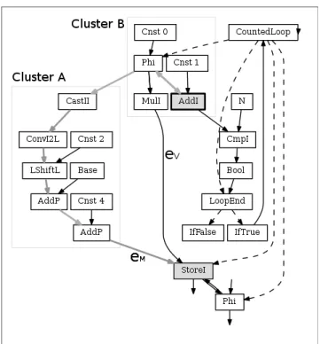
Let us consider the very simple example of listing 4,. The resulting IG for this loop is shown in figure 5. In the figure, the StoreI represents the assignment to A[i], the MulI node represents the i*i expression. The address is resolved by the nodes in the Cluster A (containing the LShift node). f o r ( i n t i = 0; i < N ; i ++ )

A [ i ] = i * i ;

Listing 4: Example loop for the implementation

3.3

Detecting Target Loops

Section 2.2 formally described the shape of loops targeted by the proposed optimization. This section describes how our implementation detects them in the IG.

Section 2.2 defined the loops Approximate Unrolling can target. Fortunately, Java for loops having a constant-increment update expression are also the target of other well known optimizations such as Range Check Elimination and Loop Unrolling. Therefore, the C2 recognizes them and marks their start using CountedLoop nodes. When our opti-mization kicks in, the compiler has already marked the loops with CountedLoop nodes, recognized the nodes belonging to the update expression and the ones belonging to the loop’s body. The compiler does this using the works of Click[11],

Figure 5: The ideal graph of the example loop of listing 4. Dashed arrows represent control edges and solid arrows represents data edges.

Vick, [40] and Tarjan [37]. Figure 5 shows the CountedLoop recognized by the C2 for the loop in listing 4. The nodes in the graph are those listed in the CountedLoop metadata. This metadata also indicates that the update expression con-tains solely the AddI node (in gray).

Once the loops with constant-increment update expression are detected, the next step consists in determining if there is an array who’s index expression value depends on the loop’s update expression. As we mentioned, the CountedLoop node maintains a list of all the nodes in its body. To determine if there is an array assignment within the loop, we look for a Store writing to memory occupied by an array. In the example of figure 5 we find the StoreI node (in gray).

Finally, we check if the array index expression value de-pends on the loop’s update expression. As the IG is a Value Dependency Graph, we look for a path of data edges be-tween the Store node representing the array assignment and any node belonging to the loop’s update expression. In the example of figure 5 this path is highlighted using bold gray edges. Thanks to the metadata stored in CountedLoop, we know that the update expression only contains the AddI node. Therefore, in the example, the path is composed of the following nodes: AddI → Phi → CastII → ConvI2L → LShiftL → AddP → AddP → StoreI.

3.4

Unrolling

Our implementation piggybacks in two optimizations al-ready present in the C2 compiler: Loop Unrolling and Range Check Removal. At the point Approximate Unrolling kicks in, the compiler has already unrolled the loop and per-formed Range Check Removal.

Figure 6: The ideal graph for the unrolled loop of listing 4 before approximating. Solid arrows represent data edges. 1 B8: # 2 movl [RCX + #16 + R9 << #2], R8 # int 3 movl R9, R10 # spill 4 addl R9, #3 # int 5 imull R9, R9 # int 6 movl R8, R10 # spill 7 incl R8 # int 8 imull R8, R8 # int 9 movl [RCX + #20 + R10 << #2], R8 # int 10 movl RDI, R10 # spill

11 addl RDI, #2 # int 12 imull RDI, RDI # int

13 movl [RCX + #24 + R10 << #2], RDI # int 14 movl [RCX + #28 + R10 << #2], R9 # int 15 addl R10, #4 # int 16 movl R8, R10 # spill 17 imull R8, R10 # int 18 cmpl R10, R11 19 jl,s 7

Listing 5: Assembler code generated for the example loop without using Approximate Unrolling

1 B7: # B8 <- B8 top-of-loop Freq: 986889

2 movl RBX, R8 # spill 3 B8: # 4 movl [R11 + #16 + RBX << #2], RCX # int 5 movl [R11 + #20 + R8 << #2], RCX # int 6 movl RBX, R8 # spill 7 addl RBX, #2 # int 8 imull RBX, RBX # int 9 movl [R11 + #24 + R8 << #2], RBX # int 10 movl [R11 + #28 + R8 << #2], RBX # int 11 addl R8, #4 # int 12 movl RCX, R8 # spill 13 imull RCX, R8 # int 14 cmpl R8, R9 15 jl,s B7

Listing 6: Assembler code for the example loop using Approximate Unrolling

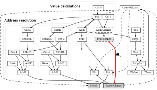
While unrolling, the compiler clones all the instructions of the loop’s body. Figure 6 shows the IG once the loop of listing 4 has been unrolled. The cloning process introduces two Store nodes: StoreI and StoreI-Cloned. Due to C2’s design, the cloned nodes belong to the even iteration of the loop. Once the loop is unrolled, Approximate Unrolling reshapes the graph to achieve the interpolated step by mod-ifying one of the two resulting iterations. Nearest Neighbor modifies the even iteration, while Linear interpolation re-shapes the odd iteration.

3.4.1

Nearest Neighbor Interpolation

As mentioned in section 3.2, a Store node takes two in-put data edges eM and eV. Edge eM links with the node

computing the memory address, while eV links with node

producing the value to write.

Approximate Unrolling performs nearest neighborhood interpolation by disconnecting the cloned Store node from the node producing the value being written (i.e. it deletes eV). In figure 6 this means to disconnect node MulI-Clone

(in gray) from node StoreI-Clone by removing edge eV.

This operation causes the node producing the value (in the example MulI-Clone) to have one less value dependency and potentially become dead if it has no other dependencies. A node without value dependencies means that its compu-tations are not being consumed and therefore is useless dead code. In this case, the node is removed from the graph. We recursively delete all nodes that do not have dependencies anymore, until no new dead nodes appear. In figure 6, we delete MulI-Cloned and then AddI-Cloned. This simplifica-tion of the IG translates into less instrucsimplifica-tions when the IG is transformed in assembler code.

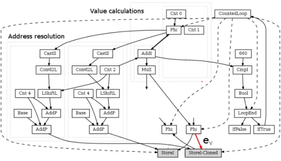
After the removal, Approximate Unrolling connects the node producing the value for the original Store into the cloned Store. Figure 7 shows the shape of the IG after Ap-proximate Unrolling has apAp-proximated the graph using nearest neighbor. Note that MulI-Clone and AddI-Clone

Figure 7: The ideal graph for the unrolled loop of listing 4 after Approximate Unrolling have modified the graph using nearest neighbor interpolation.

are deleted and that Store-Clone is connected by ev to the

same node as StoreI. The nodes producing the address re-main different.

Listing 5 shows the code generated by C2, without per-forming Approximate Unrolling: the compiler has un-rolled the loop twice, generating four storages to memory (lines 2, 3, 9, 10) and four multiplication instructions (imull, lines 5, 8, 12, 17). Listing 6 shows the code generated for the same loop using our transformation: there are still four stor-ages (lines 4, 5, 9, 10), but only two multiplications (Lines 8, 13).

3.4.2

Linear Interpolation

To unroll using linear interpolation, Approximate Un-rolling needs the first and last iteration of the loop peeled. Fortunately, this is also a requirement of other optimizations such Range Check Removal and we exploit this feature to peel the first and last iterations of the loop. The current im-plementation of the Range Check Removal creates two guard loops, one before the main loop and other after. These guard loops ensure that the main loop will not go off bounds of the array being assigned. We exploit these two guard loops for the linear interpolation.

Approximate Unrolling performs linear interpolation following a process similar to nearest interpolation. The dif-ferences are that it disconnects the value data edge evfrom

the original Store, rather than the cloned Store. This is because C2’s design implies that the cloned nodes belong to the even iteration, but linear interpolation approximates odd iterations. After the value data edge is disconnected, some nodes become dead. Here we use the same process to remove unused nodes. Finally, the interpolation is per-formed in the following way: (i) a Add node is created that receives as input the output of the cloned Store and a Phi node representing merge between the previous odd iteration of the loop and the current one (ii) a Mul node is created to multiply the result of this addition by 0.5 and this node is

connected to the the original Store effectively interpolating the loop’s even iteration.

4.

EVALUATION

To evaluate our approach, we build a version of the software-based musical synthesizer Osc3x 2_{. Using this synthesizer}

as case study, we run a series of experiments. The objective of our evaluation is twofold. First, we want to understand whether the accuracy loss caused by each optimized loop is significant or not. Second, we want to assess the benefits in performance and energy consumption of each optimized loop. We evaluate these concerns through the following re-search questions:

RQ1: Is the accuracy loss caused by the optimiza-tion to each loop acceptable?

If the accuracy loss goes to a point where the results are unacceptable there is no point in making the calculations faster. Therefore, we must carefully verify that our opti-mization reduces the accuracy only to acceptable levels. We introduce a metric in section 4.2, which is tailored to evalu-ate the accuracy of our case study.

RQ2: How big is the execution times reduction per loop?

On the other hand, without a significant increment in per-formance, reducing accuracy may not pay-off. Therefore, we must carefully assess these reductions to determine the ac-tual gains in performance. In section 4.3, we implement we use microbenchmarks to estimate the computation time of each loop.

RQ3: How big are the energy savings per loop? Just like with execution times, we expect to have energy savings in exchange of accuracy loss. We use JRALP to determine the energy consumption of each loop under study.

2_{https://www.image-line.com/support/FLHelp/html/}

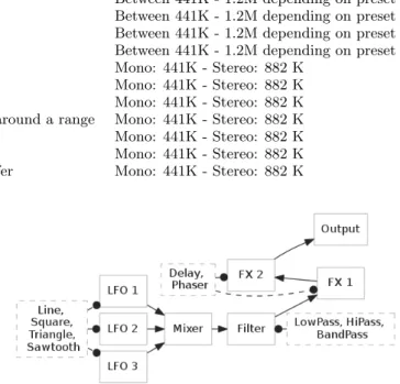
Table 1: Loops targeted by Approximate Unrolling in our case study.

Loop Function Executions in 20s (Min, Max)

A. Sine LFO Generates a sine wave. Between 441K - 1.2M depending on preset B. Triangle LFO Generates a triangular impulse Between 441K - 1.2M depending on preset C. Square LFO Generates an square impulse Between 441K - 1.2M depending on preset D. Sawtooth LFO Generates a sawtooth impulse Between 441K - 1.2M depending on preset E. Mixer Mix the LFO’s output in one signal Mono: 441K - Stereo: 882 K

F. Low Pass Filters out higher frequencies Mono: 441K - Stereo: 882 K G. High Pass Filters out lower frequencies Mono: 441K - Stereo: 882 K H. Band Pass Attenuates higher and lower frequencies around a range Mono: 441K - Stereo: 882 K I. Delay Creates a delay effect Mono: 441K - Stereo: 882 K J. Phaser Creates a phaser effect Mono: 441K - Stereo: 882 K K. Output Copies the signal to the sound card’s buffer Mono: 441K - Stereo: 882 K

4.1

Evaluation Program & Dataset

Our version of Osc3x is based on JSyn [8], a software-based musical synthesizer framework. We choose JSyn to evaluate our approach because the framework works by con-necting sound units that generate or manipulate signal us-ing loops that are good candidates for Approximate Un-rolling. The loops are usually a central piece of the Jsyn units.

As shown in figure 8, Osc3x works by mixing together the signal produced by three low frequency oscillators (LFO). The mixer’s output is then filtered using a digital biquad filter. We also added two sound effect (FX) units. The synthesizer can be configured by setting each oscillator type (Sine, Square, Triangle, Sawtooth), FX units effects (Delay, Phase), the filter type (LowPass, HiPass, BandPass) and the mixer’s LFO level. This is called a preset. The oscil-lators, mixers, FXs and filters are built-in with Jsyn, our implementation only connect them together.

For our experiments, we run Osc3x with 10 musical scores. The scores are well known tunes such as Star Wars and Su-per Mario Bros themes. Each score is played with 10 dif-ferent presets, which are designed to test all the synthesizer features.

The case study music synthesizer contains 11 loops that Approximate Unrolling can target. In all cases each loop was the central piece of code for each Jsyn unit conforming the synthesizer. Their function is described in table 1 and a letter from A to K to better represent them in figures 9, 10 and 11. The target loop are computational intensive, table 1 also shows the number of times each loop was executed to produce an arbitrary amount of 20 seconds of sound. Each loop execution counted for 10 iterations. The number of iteration is set by the JSyn engine to meet its real time requirements.

The code for our synthesizer, as well as all the microbench-marks, resulting data and rendered sound files can be found on the webpage of the Approximate Unrolling project3_.

4.2

RQ1: Accuracy Loss Assessment

To answer RQ1 we render each score using all the presets without approximating any loop. This results in 100 sound files that we use as baseline. Then, we play the same scores with the synthesizer in which we approximate one loop at a time. This produces 11 sets of 100 sound files. We then perform a pairwise comparison to assess the accuracy loss created by approximating each loop. This experiment was

3

https://github.com/approxunrollteam

Figure 8: Diagram showing how the JSyn units are connected to build our Osc3x synthesizer.

repeated twice for each loop in the synthesizer: once using the nearest neighbor and once with linear interpolation.

Notice that it is possible that a given preset causes the execution of the synthesizer not to cover the approximate loop, in such case, the resulting file is not taken into account. To compare two audio files we use the Perceptual Evalu-ation of Audio Quality (PEAQ) [42] metric. This is a stan-dard metric designed to objectively measure the audio qual-ity as perceived by the human ear. The metric was designed to compare sounds simulating the psychoacoustic of the hu-man ear, which is not equally sensible to all frequencies. PEAQ takes one reference and one test file and compares them. It assigns a scale of contiguous value to the to the test audio, depending on how well it matches the reference: 0 (non audible degradation), -1 (audible but not annoying), -2 (audible slightly annoying), -3 (annoying) -4 (completely degraded).

Results.

Figure 9 is a box plot showing the distribution of PEAQ measurements for each loop presented in Table 1 (we use the letters A to K to identify each loop). The gray boxes correspond to losses when using nearest neighbor transfor-mation while white boxes correspond to losses when using linear interpolation. Boxes corresponding to linear interpo-lation can be also identified because the letter assigned to the loop is followed by an ‘L’. This way, ‘AL’ means ‘Sine LFO interpolated with linear interpolation’.

Globally, the accuracy loss is very much acceptable and stable for each loop. The accuracy reduction for loops A, B, C, D (Sine, Sawtooth, Square and Triangle LFOs) is al-ways above the -1.5 line and in many cases over the -1 line,

Figure 9: PEAQ metric results for each approximate loop (0 to 1 - Not audible degradation; 1 to 2 - audible not annoying; 2 to 3 - slightly annoying; 3 to 4 - annoying; 4 & below - useless). Gray boxes represents loops approximated with nearest neighbor, while white boxes with linear interpolation.

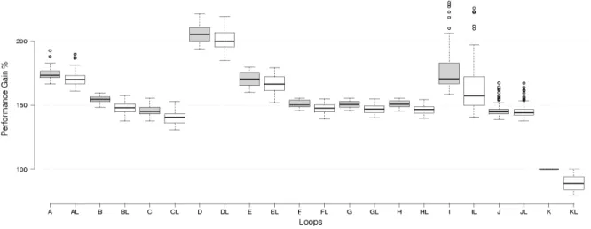
Figure 10: Performance improvement for each approximate loop. Like before, gray boxes nearest neighbor approximation and while white boxes linear interpolation.

Figure 11: Energy consumption behavior for each approximate loop. Once again, gray boxes nearest neighbor approximation and while white boxes linear interpolation.

meaning that this reduction is not significant and in many cases undetectable by the human listener. We believe there are three reasons for this good performance (i) the produced signal’s nature is benign for interpolation as indeed these are locally smooth functions (ii) there were no accumulation in the error (i.e. the results mapped to y[i] are independent of those mapped to y[i + 1]) (iii) the accuracy loss produced a harmonic distortion that was attenuated later by the syn-thesizer’s filters.

Loops F, G, H and I (representing the integrated LowPass, HighPass, BandPass filters and the Delay FX unit) appear as outliers in this experiment. The distortion was always audible and in some cases slightly annoying. We believe the main reason for this is the recursive nature of the functions governing both the filters and the delay. This accumulates error over time and eventually the resulting signal is more heavily distorted than in the case when non-recursive sig-nals are approximate using Approximate Unrolling. For example, the recursive equation (2) governs the biquad fil-ters units. Note that the resulting value y[n] depends on y[n − 1] and y[n − 2], which we believe is the cause for the bigger looses in accuracy of loops F,G and H as the error accumulates.

y[n] = b0x[v] + b1x[n − 1] + b2x[n − 2] − a1y[n − 1] − a2y[n − 2]

(2) In general, loops interpolated with the linear interpolation degrade accuracy less than those approximated using nearest neighbor with exception of the loop implementing the Square LFO. This occurs because the governing equation for this unit (y[t] = sgn(sin(t))) had the property that in most cases y[t] = y[t+1]. Therefore, the nearest neighbor approximated loop version output is frequently the same that the original one.

Loops E, J and K, representing the LFO Mixer, the Phaser FX unit and the Output also yield good results ranging from non-audible to non-annoying. The computations in these loops did not accumulate error either.

4.3

RQ2: Execution Times Reduction

To evaluate the execution times of the optimized versions of the loops, we generate one microbenchmark per loop.We run the same microbenchmark with Approximate Un-rolling turned on and off in the Virtual Machine and com-pared the execution times.

Determining whether there is an effective gain in terms of performance is a challenging task in Java [2]. We run our microbenchmarks using the statistical methodology in-troduced by George [15] to ensure that the measurements of each run were consistent. All runs where performed in an Intel i7 i7-6600U CPU, 2.60GHz with 16GB RAM running Linux Ubuntu 16.04.

Results.

Figure 10 shows the results obtained by running our mi-crobenchmark set. In all cases, the performance boost using linear interpolation was slightly smaller. This is because of the mean calculation performed in this variant of Approxi-mate Unrolling. However, compared to the computations skipped, the median computation is not so expensive and there not much difference in the performance of both opti-mizations.

All loops, except the D and K loops, run between 140%

and 180%. These is a remarkable benefit of our transforma-tion: we can succesfully increase the performance with little impact (or in some cases none) on the quality of the signal. Loop D runs 200% faster than the original version. This is because its body is mainly composed of arithmetical op-erations only, which our implementation is very efficient re-moving.

It is interesting to notice that the optimized loop K (Out-put) actually runs slower. The accurate loop K simply copies the value of an array to another array. Therefore, the oper-ations removed from the body are not more time consuming than the operations added by the nearest neighbor transfor-mation and are even less time consuming than all computa-tions added in the case of the linear interpolation.

4.4

RQ3: Energy savings

We evaluate our energy savings by estimating the total energy consumption of our microbenchmarks using JRALP [19], a Java library that exposes to Java programs the the In-tel’s Running Average Power Limit (RAPL) Technoolgy [1]. We first run the microbenchmark set and estimate energy consumption without optimizing any loop with Approxi-mate Unrolling. In a second step, we repeated the exper-iment, this time turning the proposed optimization on and compared the energy consumption estimates of both runs.

Results.

The results displayed in figure 11 indicate a clear reduc-tion in energy consumpreduc-tion for most loops. In general, most loops are able to reduce their consumption within 50% - 70 % range. Also, the transformation based on linear inter-polation is less energy effective than nearest neighbor as it introduces a few more computations. Again, loop K was the counter example, as the optimization introduced more operations that the one it was able to remove.

5.

DISCUSSION

Section 4 shows promising results as they indicate that Approximate Unrolling can actually reduce the execu-tion times and energy consumpexecu-tion of optimized loops with-out a significant impact in the signal’s quality.

We choose to keep the data set small (11 loops), enabling us to provide a per-case analysis on the impact of the trans-formation on each loop and to understand the reasons be-hind the improvement (or not) in each case. The lessons learned on this case study drive the future work, as we now have a better understanding of which loops should gain more of the optimization. Loop K got its performance reduced because Approximate Unrolling interpolations were ac-tually more expensive than the original loop. On the other hand, the LFO loops ran significantly faster and with less energy, without significant impact on the signal’s quality. We learned that this was due to the non-recursiveness and smoothness of the function being mapped to the array, as well as the capacity of the system being approximate (the Osc3x synthesizer) to absorb the accuracy loss.

As with other approximate computing techniques, Ap-proximate Unrolling is effective in domains where some degree of inexactitude can be allowed, e.g. as video and sound, numerical simulations and games. We have evalu-ated Approximate Unrolling using a single domain of application. This certainly raises the question of the ap-plicability of Approximate Unrolling outside the field of

sound. However, sound signals share many properties with other time series data such as sensor readings, stock share values and even video. Therefore, we believe Approximate Unrolling could be exploited in other domains as well.

Our results suggest that the situations in which Approx-imate Unrolling will work best are those in which the data stored close to each other in memory are also logically re-lated to each other in the application’s data model. This is the case in numerous data representations, like sound, trian-gle strips, sensor data, market trends, etc. For example, in sensor data (such as sound recoding and weather) two con-secutive array elements will represent two readings close to each other in time; in 3D visualizations, triangles topologi-cally close to each other will be stored in contiguous array slots.

Threads to validity.

We did extensive testing of our code and reviewed our mi-crobenchmarks using best practices for microbenchmarking [15, 2]. However, Java microbenchmarking is a very diffi-cult craft [2] and is possible to overlook a details skeweding the measurement. Also, the Hotspot’s C2 is a very complex piece of code. We introduced a modification to this software and there may be bugs. We hope that if such is the case, they have only a marginal quantitative impact, and not distort the qualitative essence of our findings. Our infrastructure is publicly available on Github.

6.

RELATED WORK

The quest for energy savings and performance has made Approximate Computing an attractive research direction in the last few years[25], [41], [29]. The approaches are numer-ous and diverse, as they use hardware, software or a mixture of both.

Hardware-oriented approximation techniques have proposed hardware components with approximation capabilities, such as FPUs that dynamically adapts the mantissa width [38], approximate adders [16, 33], memory designs that exploit voltage scaling [10, 18] or that allow bit flipping [20]. Also, general circuit design techniques has been proposed to ex-ploit the accuracy-performance trade-off [5, 27, 39]. Another trend is to take advantage of an existing non-determinism of the hardware [21, 32, 35] or expose it to the developers to let them exploit it [7, 36].

On the other hand, software-oriented techniques proposes ways to approximate existing algorithms automatically [34, 24, 22, 28, 31] or provides support for programming using approximation [4, 6, 23, 30, 9].

Closest to our technique is Loop Perforation[34], which skip some iteration of the loop or terminate it early. Loop Perforation and Approximate Unrolling differs in the scope where they can best applied, as well in the trans-formation made to the code. Loop Perforation works better in patterns that can completely skip some task, like Monte-Carlo simulations, computations iteratively improving an al-ready obtained result or explorations to filter or select ele-ments in a given search space. Approximate Unrolling do not skips any iteration of the loop, instead, it replaces the computations of some iterations by approximate ones. Approximate Unrolling best results are obtained when applied in loops mapping values to arrays and works good even if no previous value was mapped before. By construc-tion, it behaves better than Loop Perforation in situations

when no value of the array can be left undefined.

Another related technique to Approximate Unrolling is the Paraprox framework [28]. Paraprox works by detect-ing and proposdetect-ing approximate alternative to patterns in parallel applications. One of the detected patters (stencil) also works on the assumption that nearby array elements are similar in image and video applications. Paraprox ex-ploits this to skip memory accesses. Approximate Un-rolling and Paraprox diverge in the sense that Paraprox uses the neighbor similarity to avoid memory accesses, while Approximate Unrolling uses it to avoid computations. The stencil pattern in Paraprox is also fine-tuned for Ma-trix arrays (images, videos), which is not the representation of sound or times series. This set apart both approaches w.r.t. the type of data each one is better suited for.

There are a number of approaches allowing the program-mer to provide multiples alternatives to the same algorithm [6, 4]. In this context, Approximate Unrolling can be used as a way to provide one of such alternatives where ac-curacy can be exchanged for performance or energy savings. Similarly, several languages have been designed to indicate the parts of a program that can be approximate. Examples of this are EnerJ[30], FlexJava[26] and Rely[9]. Separat-ing the parts of a program that can be approximate is an orthogonal concern to Approximate Unrolling. In our experiments we used EnerJ annotations to select one loop to approximate out of all the loops our optimization could target in the entire program, allowing us to assess the impact of a single loop each time and showing that our technique is indeed complementary with these approximate languages.

7.

CONCLUSIONS & FUTURE WORK

In this paper we have described Approximate Unrolling, an a transformation that approximates the computation in-side certain loops. We formally described the shape of the loops selected for Approximate Unrolling, as well as the transformations it performs to reduce execution times and energy consumption at the expenses of accuracy loss. We have also proposed an implementation of this transforma-tion inside the OpenJDK Hotspot C2 Server compiler.

The empirical assessment of this transformation on the loops of the JSyn sound library demonstrated the ability of Approximate Unrolling to effectively trade accuracy for resource gains. We learned that not all loops respond equally well to the approximation and we gained some in-sights on the causes for this. Hence, our future work will consist in including these findings into the optimization, im-proving the detection process using a cost function that fa-vors loops whose bodies (i) contains more instructions than the ones introduced by Approximate Unrolling (ii) have a minimal number of instructions depending on a value cal-culated in a previous iteration (iii) represents an smooth function. Then, the selection will filter out those loops be-low a given threshold of the cost function.

Another direction in the future is to assess the applicabil-ity of Approximate Unrolling in other domains. We fo-cused this work on a single case study to gain precise insights about the nature of loops that can benefit from Approxi-mate Unrolling. Yet, in future work we will evaluate the impact of approximating more loops and more iterations in each loop.

8.

REFERENCES

[1] Intel ˆA˝o 64 and IA-32 Architectures Developer’s Manual.

[2] Aleksey Shipilev. Necessar(il)y Evil dealing with benchmarks, ugh, July 2013.

[3] J. R. Allen, K. Kennedy, C. Porterfield, and

J. Warren. Conversion of Control Dependence to Data Dependence. In Proceedings of the 10th ACM

SIGACT-SIGPLAN Symposium on Principles of Programming Languages, POPL ’83, pages 177–189, New York, NY, USA, 1983. ACM.

[4] J. Ansel, C. P. Chan, Y. L. Wong, M. Olszewski, Q. Zhao, A. Edelman, and S. P. Amarasinghe. PetaBricks: a language and compiler for algorithmic choice. In ACM Conference on Programming Language Design and Implementation (PLDI), 2009.

[5] L. Avinash, C. C. Enz, J.-L. Nagel, K. V. Palem, and C. Piguet. Energy parsimonious circuit design through probabilistic pruning. In Design, Automation and Test in Europe (DATE), 2011.

[6] W. Baek and T. M. Chilimbi. Green: A framework for supporting energy-conscious programming using controlled approximation. In ACM Conference on Programming Language Design and Implementation (PLDI), 2010.

[7] J. Bornholt, T. Mytkowicz, and K. S. McKinley. Uncertain\textlessT\textgreater: A First-Order Type for Uncertain Data. In International Conference on Architectural Support for Programming Languages and Operating Systems (ASPLOS), 2014.

[8] P. Burk. JSyn - A Real-time Synthesis API for Java. In Proceedings of the International Computer Music Conference, pages 252–255. International Computer Music Association, 1998.

[9] M. Carbin, S. Misailovic, and M. C. Rinard. Verifying Quantitative Reliability for Programs that Execute on Unreliable Hardware. In ACM Conference on

Object-Oriented Programming, Systems, Languages, and Applications (OOPSLA), 2013.

[10] I. J. Chang, D. Mohapatra, and K. Roy. A

Priority-Based 6t/8t Hybrid SRAM Architecture for Aggressive Voltage Scaling in Video Applications. IEEE Transactions on Circuits and Systems for Video Technology, 21(2):101–112, 2011.

[11] C. Click. Global Code Motion/Global Value Numbering. In Proceedings of the ACM SIGPLAN 1995 Conference on Programming Language Design and Implementation, PLDI ’95, pages 246–257, New York, NY, USA, 1995. ACM.

[12] C. Click and M. Paleczny. A Simple Graph-based Intermediate Representation. In Papers from the 1995 ACM SIGPLAN Workshop on Intermediate

Representations, IR ’95, pages 35–49, New York, NY, USA, 1995. ACM.

[13] K. D. Cooper and L. Torczon. Engineering a Compiler. Morgan Kaufmann, 2005.

[14] J. Ferrante, K. J. Ottenstein, and J. D. Warren. The Program Dependence Graph and Its Use in

Optimization. ACM Trans. Program. Lang. Syst., 9(3):319–349, July 1987.

[15] A. Georges, D. Buytaert, and L. Eeckhout.

Statistically Rigorous Java Performance Evaluation.

In Proceedings of the 22Nd Annual ACM SIGPLAN Conference on Object-oriented Programming Systems and Applications, OOPSLA ’07, pages 57–76, New York, NY, USA, 2007. ACM.

[16] V. Gupta, D. Mohapatra, S. P. Park,

A. Raghunathan, and K. Roy. IMPACT: Imprecise adders for low-power approximate computing. In International Symposium on Low Power Electronics and Design (ISLPED), 2011.

[17] S. Kulkarni and J. Cavazos. Mitigating the Compiler Optimization Phase-ordering Problem Using Machine Learning. In Proceedings of the ACM International Conference on Object Oriented Programming Systems Languages and Applications, OOPSLA ’12, pages 147–162, New York, NY, USA, 2012. ACM.

[18] A. Kumar, J. Rabaey, and K. Ramchandran. SRAM supply voltage scaling: A reliability perspective. In International Symposium on Quality Electronic Design (ISQED), 2009.

[19] K. Liu, G. Pinto, and L. Yu David. Data-Oriented Characterization of Application-Level Energy Optimization. 2015.

[20] S. Liu, K. Pattabiraman, T. Moscibroda, and B. G. Zorn. Flikker: Saving Refresh-Power in Mobile Devices through Critical Data Partitioning. In International Conference on Architectural Support for Programming Languages and Operating Systems (ASPLOS), 2011. [21] C. Luo, J. Sun, and F. Wu. Compressive Network

Coding for Approximate Sensor Data Gathering. In IEEE Global Communications Conference

(GLOBECOM), 2011.

[22] L. McAfee and K. Olukotun. EMEURO: A Framework for Generating Multi-purpose Accelerators via Deep Learning. In International Symposium on Code Generation and Optimization (CGO), 2015.

[23] S. Misailovic, M. Carbin, S. Achour, Z. Qi, and M. C. Rinard. Chisel: Reliability- and Accuracy-aware Optimization of Approximate Computational Kernels. In ACM Conference on Object-Oriented Programming, Systems, Languages, and Applications (OOPSLA), 2014.

[24] S. Misailovic, D. Kim, and M. Rinard. Parallelizing Sequential Programs With Statistical Accuracy Tests. Technical Report MIT-CSAIL-TR-2010-038, MIT, Aug. 2010.

[25] S. Mittal. A Survey of Techniques for Approximate Computing. ACM Comput. Surv., 48(4):62:1–62:33, Mar. 2016.

[26] J. Park, H. Esmaeilzadeh, X. Zhang, M. Naik, and W. Harris. FlexJava: Language Support for Safe and Modular Approximate Programming. In Proceedings of the 2015 10th Joint Meeting on Foundations of Software Engineering, ESEC/FSE 2015, pages 745–757, New York, NY, USA, 2015. ACM.

[27] A. Ranjan, A. Raha, S. Venkataramani, K. Roy, and A. Raghunathan. ASLAN: Synthesis of Approximate Sequential Circuits. In Design, Automation and Test in Europe (DATE), 2014.

[28] M. Samadi, D. A. Jamshidi, J. Lee, and S. Mahlke. Paraprox: Pattern-based Approximation for Data Parallel Applications. In International Conference on Architectural Support for Programming Languages and

Operating Systems (ASPLOS), 2014.

[29] A. Sampson. Approximate Computing: An Annotated Bibliography, 2016.

[30] A. Sampson, W. Dietl, E. Fortuna,

D. Gnanapragasam, L. Ceze, and D. Grossman. EnerJ: approximate data types for safe and general low-power computation. In ACM Conference on Programming Language Design and Implementation (PLDI), 2011. [31] E. Schkufza, R. Sharma, and A. Aiken. Stochastic

Optimization of Floating-Point Programs with Tunable Precision. In ACM Conference on

Programming Language Design and Implementation (PLDI), 2014.

[32] S. Sen, S. Gilani, S. Srinath, S. Schmitt, and S. Banerjee. Design and implementation of an ”approximate” communication system for wireless media applications. In ACM SIGCOMM, 2010. [33] M. Shafique, W. Ahmad, R. Hafiz, and J. Henkel. A

Low Latency Generic Accuracy Configurable Adder. In Design Automation Conference (DAC), 2015. [34] S. Sidiroglou-Douskos, S. Misailovic, H. Hoffmann,

and M. C. Rinard. Managing performance vs. accuracy trade-offs with loop perforation. In ACM SIGSOFT Symposium on the Foundations of Software Engineering (FSE), 2011.

[35] P. Stanley-Marbell and M. Rinard. Approximating

Outside the Processor. 2015.

[36] P. Stanley-Marbell and M. Rinard. Lax: Driver Interfaces for Approximate Sensor Device Access. In USENIX Workshop on Hot Topics in Operating Systems (HotOS), 2015.

[37] R. Tarjan. Testing flow graph reducibility. [38] J. Y. F. Tong, D. Nagle, and R. A. Rutenbar.

Reducing power by optimizing the necessary precision/range of floating-point arithmetic. IEEE Transactions on Very Large Scale Integration (VLSI) Systems, 8(3), 2000.

[39] S. Venkataramani, K. Roy, and A. Raghunathan. Substitute-and-simplify: A Unified Design Paradigm for Approximate and Quality Configurable Circuits. In Design, Automation and Test in Europe (DATE), 2013.

[40] C. A. Vick. SSA-based reduction of operator strength. Thesis, Rice University, 1994.

[41] Q. Xu, T. Mytkowicz, and N. S. Kim. Approximate Computing: A Survey. IEEE Design Test, 33(1):8–22, Feb. 2016.

[42] M. ˚A˘aalovarda, I. Bolkovac, and H. Domitrovi ¨A ˘G. Estimating perceptual audio system quality using PEAQ algorithm. In ICECom (18; 2005), 2005.