HAL Id: hal-00761668
https://hal.archives-ouvertes.fr/hal-00761668
Submitted on 25 Jun 2019
HAL is a multi-disciplinary open access
archive for the deposit and dissemination of
sci-entific research documents, whether they are
pub-L’archive ouverte pluridisciplinaire HAL, est
destinée au dépôt et à la diffusion de documents
scientifiques de niveau recherche, publiés ou non,
Investigation on the Effort Transmission in Planar
Parallel Manipulators
Sébastien Briot, Victor Glazunov, Vigen Arakelian
To cite this version:
Sébastien Briot, Victor Glazunov, Vigen Arakelian. Investigation on the Effort Transmission in
Pla-nar Parallel Manipulators. Journal of Mechanisms and Robotics, American Society of Mechanical
Engineers, 2013, 5 (1). �hal-00761668�
Sébastien Briot
Institut de Recherches en Communications et Cybernétique de Nantes (IRCCyN), Nantes, France
Victor Glazunov
Mechanical Engineering Research Institute Russian Academy of Sciences Moscow, Russia [email protected]
Vigen Arakelian
Institut National des Sciences Appliquées (INSA), Rennes, France Département de Génie Mécanique et Automatique [email protected]
Investigation on the Effort
Transmission in Planar
Parallel Manipulators
In the design of a mechanism, the quality of effort transmission is a key issue. Traditionally, the effort transmissivity of a mechanism is defined as the quantitative measure of the power flowing effectiveness from the input link(s) to the output link(s). Many researchers have focused their work on the study of the effort transmission in mechanisms and diverse indices have been defined. However, the developed indices have exclusively dealt with the studies of the ratio between the input and output powers and they do not seem to have been devoted to the studies of the admissible reactions in passive joints. However, the observations show that is possible for a mechanism to reach positions in which the transmission indices will have admissible values but the reaction(s) in passive joint(s) can reach excessively high values leading to the breakdown of the mechanism. In the present paper, a method is developed to ensure the admissible values of reactions in passive joints of planar parallel manipulators. It is shown that the increase of reactions in passive joints of a planar parallel manipulator depends not only on the transmission angle but also the position of the instantaneous centre of rotation of the platform. It allows the determination of the maximal reachable workspace of planar parallel manipulators taking into account the admissible reactions in its passive joints. The suggested method is illustrated vie a 5R planar parallel mechanism and a planar 3-RPR parallel manipulator.
I Introduction
Parallel manipulators have many advantages in terms of acceleration capacities and payload-to-weight ratio [1], but one of their main drawbacks concerns the presence of singularities [2]– [5]. It is known that in the neighbourhood of the singular positions the reactions in joints of a manipulator considerably grow up.
In order to have a better understanding of this phenomenon, many researchers have focused their works on the analysis of the effort transmission in parallel manipulators. One of the evident criterions for evaluation of effort transmission is the transmission angle (or pressure angle which is equal to 90 degrees minus the transmission angle) [7]–[9]. The pressure angle is well known for characterizing the transmission quality in lower kinematic pairs, such as cams [10], but this idea was also used for effort transmission analysis in the parallel manipulators [7], [9].
To evaluate the effort transmission quality, several indexes have been introduced. One of the first attempts was proposed in [6]. This paper presents a criterion named the Transmission Index (TI) that is based on transmission wrench screw. The TI varies between 0 and 1. If it is equal to 0, the considered link is in a dead position, i.e. it cannot move anymore. If it is equal to 1, this link has the best static properties.
In the same vein as [6], the study [11] generalizes the TI for spatial linkages and defines the Global TI (GTI). The authors also prove that the GTI is equal, for prismatic and revolute joints, to the cosine of the pressure angle.
The conditioning index was also proposed [12] for characterizing the quality of transmission between the actuators and the end-effector. This index is based on the Jacobian matrix or its “norm”, which relate the actuator velocities (efforts, resp.) to the platform twist (wrench, resp.) by the following relations:
t Jq and w J τ , where J is the Jacobian matrix, t the T
platform twist, q the input velocities, the actuator efforts, and
w the wrench applied on the platform.
All these indices have been used in many works for design and analysis of parallel mechanisms [14]–[21]. However, it is also known that because of the non homogeneity of the terms of the Jacobian matrix, the conditioning index is not well appropriated for mechanisms having both translational and rotational degrees of freedom (DOF) [13]. Moreover, all the previously mentioned indices do not take into account the real characteristics of the actuators, i.e. the fact that their input efforts are bounded between [– max
i
, max
i
] [13].
In order to solve this problem, in study [22] a numerical analysis method has been developed. It has been proposed to characterize the force workspace of robots taking into account a given fixed wrench applied on the platform and actuator efforts comprised in the boundary interval [–imax,imax]. However, this
workspace depends on the given direction and norm of the external force/moment and will change with the variation of the applied wrench. Moreover, for many robot applications, the external wrench direction is not known, contrary to its norm. Therefore, in [23], a way to compute the maximal workspace
taking into account the actuator effort limitations for a given norm of the external force and moment was proposed. This approach is based on the computation of the transmission factors of matrix J–
T, which are obtained geometrically through the mapping of a
cube by the Jacobian matrix.
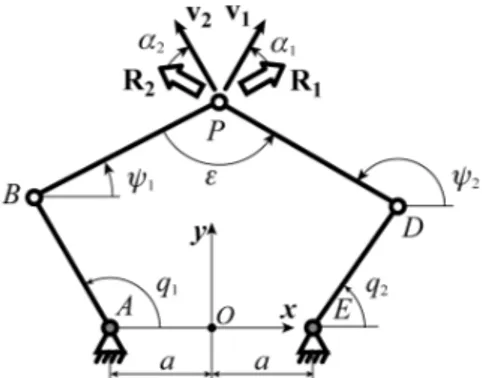
All the previously mentioned approaches analyse the quality of the effort transmission by taking into account the input torque limitations only. However, there are such positions of parallel manipulators for which the limitations of input torques can be satisfied and the limitation of reactions in passive joints not at all. To have a better understanding of this phenomenon, let us consider a simple example via a planar 5R manipulator (Fig. 1). Close to such singularity a small effort w applied on the end-effector of the manipulator will create a large reaction R1 in the
passive joint B. But in this pose, the actuator torques 1 will stay
under acceptable values, as it depends only on the small component F1 of the reaction R1. Thus, for the mentioned case,
the transmission indices will have acceptable values but they will not give any information about the inadequately high values of reactions in passive joints of the mechanism.
Therefore, the development of criteria for limitation of the passive joints’ reactions is also an important consideration in effort transmission field. It is a complementary condition to the transmission indices for characterizing the quality of effort transmission especially in the neighbourhood of singularity.
This paper focuses on the study of the effort transmission in planar parallel mechanisms (PPM) from the above point of view. It aims at proposing a new criterion for taking into account the passive joint reactions and at finding the relationships between this criterion and the previously developed indices, especially the transmission angle.
First, the expressions of the maximal platform joint reactions as a function of the parameters of the wrench applied on the platform is presented, i.e. the maximal force norm and the absolute value of the moment. Then, it is disclosed that the maximal values of platform joint reactions depend not only the value of the transmission angle but also the position of the instantaneous centre of rotation of the platform. Moreover, the obtained results allow one to define the ranges for the admissible values of the transmission angles and distance to the instantaneous centre of rotation that ensure a good effort transmission quality. Finally, two illustrative examples and simulation results are presented.
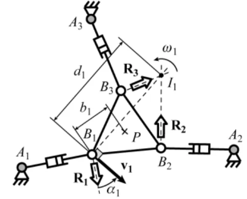
II. A criterion for evaluation of the passive joints reactions
For any PPM, the reaction forces Ri in the platform passive joints
(denoted as Bi in Fig. 2, i = 1, …, 3) can be related to the external
wrench wT = [fT, C]T (f is the external force, and C the scalar
value of the external moment applied on the platform) applying the Newton-Euler equations at any point Q:
3 1 i i
f R and 3 1 T QBi i i C
d R (1) where T [ , ]QBi yQBi xQBi
d , with xQBi and yQBi are the coordinates
of vector QBi along x and y axes (the position of point Bi may
vary if the passive joints linked to the platform are prismatic
Fig. 1. Planar 5R manipulator close to a Type 2 singular pose.
Fig. 2. Determination of the pressure angle for the planar 3-RPR robot.
joints). It should be mentioned that in Fig. 2 and the followings, the double arrows indicates the direction of the platform reaction forces, not their norm. Considering that Ri = Ri ri, where ri is a
dimensionless unit vector and ||Ri|| = Ri, and applying the
Newton-Euler equations at point B1, it comes that:
1 2 1 3 1 2 3 0 T T B B B B T R R R 1 2 3 2 3 w1 w2 w3 r r r w d r d r s s s R A R (2) 1 , i T T T i i B B i w
s r d r being unit screws corresponding to the
direction of the platform joint reaction wrenches.
Matrix A used in equation (2) is defined in [1][3] as the parallel Jacobian matrix than can be found through the differentiation of the loop closure equations of the robot with respect to the platform coordinates. As a result, this matrix is always invertible if the robot is not in a Type 2 singularity.
The reactions R of the passive joints can be found from (2):
T
R A w (3)
where matrix A–1 can be expressed in the form [2]: 1 t1 t2 t3 A s s s ,with T [ T, ] i i i t s v (4)
where sti is a screw corresponding to the direction of the platform
twist when leg i is disconnected. Moreover, it should be noted that:
- vi is a dimensionless vector parallel to the platform
translational velocity vector vBi expressed at point Bi, i.e. vBi =
- i is a scalar that is related to the platform rotational velocity
i by i = λi [7] (Fig. 2). Therefore, the dimension of i is
in m-1. On Fig. 2, point I1 corresponds to the position of the
instantaneous centre of rotation of the platform when leg 1 is disconnected.
Without loss of generality, let us consider the norm R1 of the
reaction force in the joint attaching the leg 1 to the platform (located at B1). Developing (3), it comes that:
1 T 1( TB P1 ) ( T 1 TB P1 ) 1
R v f1 Cd f v1 d f C
. (5) For a given norm f of the external force f and a given value C of the external moment, and for any direction of vector f, the maximal value R1max of R1 appears when
1max 1 , 2 2 1 1 1 1 1 1 max( ) 2 cos C R R f b b C f 1 1 v v (6) where b1 is the distance between the application point of theexternal wrench, denoted as P, and point B1. 1 is the angle
between vectors v1 and d1 B P1 (Fig. 3).
Generalizing the approach to the other legs (i = 1, 2, 3):
2 2
max max( ), 2 cos
i C i i i i i i i i i
R R f b b C
f v v . (7)
Equation (7) characterizes the effort transmission between the external wrench applied on the platform and the reaction of the platform joint located at Bi. For a given mechanism configuration
and a given value of Rimax, it is thus possible to find the
admissible ranges for f and C, i.e. for the parameters of the external wrench applied on the platform. Moreover, in order to avoid the breakdown of the platform joint located at Bi,
technological requirements must imply that the admissible value of Ri should not be superior to a given value Radm, i.e.
max
i adm
R R .
It is shown in the following section that (7) can be related to the value of the pressure angle (the pressure angle is equal to 90 deg minus the transmission angle) but, also, to the value of the distance of the platform instantaneous centre of rotation Ii when
leg i is disconnected.
III. Relationships between the maximal passive joint reaction and the pressure angle
By combining (2) and (4), it comes that T T 1
w1 t1 1 1 s s r v . Moreover, it was shown in [7] that the pressure angle of the leg 1, depicted as 1 (see Fig. 2), may be expressed as the acute angle
between the directions of vectors r1 and v1[24]. Therefore, if B1 does not coincide with I1:
1 1 cos T 1 1 1 1 r v r v , i.e. cos 1 T 1 1 1 1 r v r v (8)
By definition, r1 is a unit vector. As a result,
cos1
1
1
v .
Moreover, from the definition of a planar displacement for a rigid body, v1 d11 , where d1 is the distance from the platform
instantaneous centre of rotation I1 to point B1 (Fig. 2). Introducing
these expressions into (6), it comes that
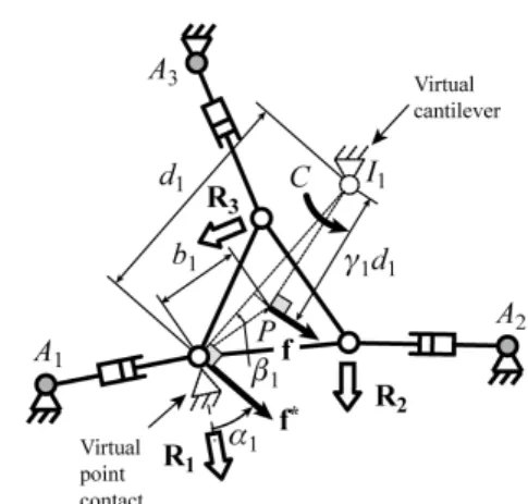
Fig. 3. Instantaneous system equivalent to the planar 3-RPR robot platform.
2 1 1 1 1 1 1 1max 1 1 / 2cos / / cos b d b d f C d R , for d1>0 (9a) 1max 1( 1 ) R f b C , for d1=0 (9b)Generalizing the approach to the other legs (i = 1, 2, 3):
max / cos i i i i f C d R , for di > 0 (10a) max ( ) i i i R f b C , for di = 0 (10b)
where i 1
b di/ i
22cosi b di/ i, di is the distancebetween point Bi and the instantaneous centre of rotation of the
platform when leg i is disconnected, i is the pressure angle of the
leg i, bi is the distance between P and Bi, and i is the angle
between vectors vi and di BiP (and as a result between vectors
BiP and BiIi – Fig. 3), dBiP, vi and i being defined at (1) and (4).
It should be mentioned that the distance between point P and Ii is
equal to idi.
Equation (10) shows that, for a given set of external force and moment applied on the platform and for di > 0, the reactions in
passive joints depend not only on the pressure angle but also the position of the instantaneous centre of rotation of the platform when one of the leg is disconnected. To the best of our knowledge, this property has not been rigorously formulated and demonstrated before. It allows not only giving a qualitative evaluation of the effort transmission in PPM but also disclosing the geometrical interpretation of the problem: from the equation (10a), it can be shown that the mechanical system under study can be instantaneously replaced by a virtual cantilever attached to the ground at Ii (Fig. 3) lying on a virtual point contact at Bi, of
which direction is parallel to the vector Ri. The external force f is
applied on the point P of the cantilever.
As i is a criterion used for the kinetostatic design of robots
[9], [14], [18],[21], it is of interest to find its boundaries with respect to the technological requirements that imply that the admissible reaction Ri in passive joints should not be superior to a
The following of the paper focused on finding the ranges on i
and di, di > 0, i.e. the parameters of the equivalent cantilever
system, for which this inequality RimaxRadm is respected.
The case di = 0 is discarded as the pressure angle cannot be
defined. However, it can be shown that the joint reaction stays under acceptable value if and only if i(f biC)Radm.
Introducing (10a) into the inequality RimaxRadm leads to:
21 i/ i 2cos i i/ i admcos i / i
f b d b d R C d . (11)
Please note that, as by definition, f, cos i, di and Radm have
positive values, a necessary condition for the existence of (11) is: 0RadmcosiC d/ i cos i
adm i
C d
R . (12)
If not, the left term of (11) will always be superior to Radm. Let
us now square the left and right sides of equation (11) and multiply them by 2 i d (from (10a), di > 0):
2 2 2 2 2 2 2cos cos 2 cos i i i i i i adm i i adm i f d b b d d R C d C R (13)The obtained expression can be rewritten as:
0p di( )i , (14) where, ( ) 2 i i i i i i i p d u d v d w, 2 cos2 2 i adm i u R f ,
2
2 cos cos i adm i i i v C R b f , 2 2 2 i i w C f b .The inequality (14) has different solutions, depending on the vanishing and signs of terms ui, vi and wi. There are three main
cases ui > 0, ui < 0 and ui = 0. Let us consider these cases.
A. ui > 0
ui > 0 implies that f Radmcosi. In this case, the polynomial
pi has got two roots but only one corresponds to the real
mechanism, i.e. to a solution of (11). The other root is solution of:
2 2 2 2 2cos 2 cos 2 2 cos i i i i i i adm i i adm i f d b b d d R C d C R (15)In order to obtain a root of (14) with physical values, it is necessary that the condition 2 4 0
i i i
v u w is respected, i.e
2 2 2
2
2
2 2 4 2 2
cos 2 cos cos
sin 0 adm i i adm i i i i i R f b C R b f b f f C (16)
Developing and simplifying, it can be shown that this polynomial in cos i has roots with real values if and only if:
2 sin2 2 4 0
adm i i i
R b f w . (17)
For the analysis of this inequality, two following cases must be considered: wi ≤ 0 and wi > 0.
A1. wi > 0
The condition wi > 0 implies that C > f bi. Here, (16) has no
real roots, i.e. (16) is true for any value of i. Thus, the condition
for (11) to be true is that
1
max , / cos i i adm i d d C R . (18) where
2
1 4 2 i i i i i i d v v u w u is the root of (14) solution of (11). A2. wi ≤ 0The condition wi ≤ 0 implies that C ≤ f bi . (16) is true if its
roots are bounded by
2 2 2 cos sin cos i i i i adm i C f b C R b (19a) or 2 2 2 cos sin cos i i i i adm i C f b C R b (19b)
After mathematical simplifications, it can be proven that if (19b) is true, then, cos i adm i adm C f R b R . (20)
which is in contradiction with ui > 0. Therefore, the only
condition for (16) to be true is that
2 2 2 cos sin cos i max i i i , adm i adm C f b C f R b R (21) However, it can be demonstrated, by studying the sign of the
function cos sin 2 2 2
i i i i gC f b C fb, that 2 2 2 cos i sin i i adm i adm C f b C f R b R , for ui > 0 and wi ≤ 0. (22)
Thus (21) implies that ui > 0, which is true. Then, (16) is always
true is this section. As a result, the only condition for (11) to be true is (18).
B. ui < 0
ui < 0 implies that f Radmcosi. Introducing this into (11)
leads to 0 ≤ i ≤ 1, i.e. the cantilever allows decreasing the applied
force f. Here also, two cases of coming from the analysis of (17) should be studied, i.e.: wi ≤ 0 and wi > 0.
B1. wi > 0
If wi > 0, i.e. C > f bi, from (12) it can be shown that:
cos cos i i adm i adm i C fb d R R . (23)
As in section II.B ui < 0, which is equivalent to Radm cos i < f,
from (23) it comes cos i i adm i fb b R , thus bi . (24) di
If (24) is true, the expression of i at (10a) is bounded by
0 i i i i i i i b d d b d d . (25)
i i
i
i i
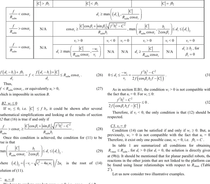
cos adm i i i f d b C f d b fb f R d d . (26) Thus, cos adm i fR , or equivalently ui > 0, (27)which is impossible in section B. B2. wi ≤ 0
If wi ≤ 0, i.e. C ≤ f bi, it could be shown after several
mathematical simplifications and looking at the results of section A2 that (16) is true if and only if
2 2 2 cos sin cos i i i i adm adm i C f b C f R R b . (28)
Once this condition is achieved, the condition for (11) to be true is that
2 max , cos 2cos i i i adm i i C b d d R . (29) where
2
2 4 2 i i i i i i d v v u w u is the root of (14) solution of (11). C. ui = 0We have to analyze one last case: ui = 0, i.e. cos i f R/ adm.
Here also, this condition leads to 0 ≤ i ≤ 1, i.e. the cantilever
allows decreasing the applied force f. In such a case, the solution
of (14) is solution of 0v di iwi with vi2f
cosi ib fC
and 2 2 2
i i
w C f b .
Three cases will appear: vi > 0, vi < 0 and vi = 0.
C1. vi > 0
In this case, RimaxRadm can be satisfied if and only if
2 2 2 2 cos i i i i i i w f b C d v f b f C . (30) C2. vi < 0In this case, RimaxRadm can be satisfied if and only if
2 2 2 0 2 cos i i i i i i w f b C d v f b f C . (31)As in section II.B1, the condition wi > 0 is not compatible with
the fact that ui = 0. For wi ≤ 0:
2 2 2 0 2 cos i i i f b C f b f C . (32)Therefore, if vi < 0, the only condition is that (12) should be respected.
C3. vi = 0
Condition (14) can be satisfied if and only if wi ≥ 0. But, as
previously, wi > 0 is not compatible with the fact that ui = 0.
Therefore, it exist only one possible case, wi = 0, i.e. fbi . C
In table 1 are summarized all conditions for obtaining
max
i adm
R R , for di > 0 (for di = 0, the solution is directly given
at (9b)). It should be mentioned that for planar parallel robots, the reactions in the other joints that are not linked to the platform can be found using linear relationships with respect to Rimax (Table
21).
Let us now consider two illustrative examples.
IV. Illustrative examples
Let us now consider, for given external wrenches, the evolution of the maximal joint reactions within the workspace of two given planar robots: the DexTAR robot, which is a planar five-bar mechanism developed at the ETS [25], and a 3-RPR robot, which is the planar model of the PAMINSA manipulator developed at the INSA of Rennes [26].
A. The DexTAR robot
The DexTAR is a five-bar mechanism [27] (Fig. 4) of which dimensions are:
- lAB = lDE = lAB = lDE = 0.23 m
1 In this table, the joints depicted in grey correspond to the actuated ones.
Table 1. Conditions for limiting the maximal values of the revolute joint linked to the platform, for di > 0.
i C fb C fbi C fbi cos i adm f R i max
i 1, cos adm i C d d R cos i adm f R N/A 2 2 2 cos sin cos i i i i adm i C f b C R b ,max ,
2 cos 2cos i i i adm i i C b d d R cos i adm f R N/A vi > 0 vi < 0 vi = 0 vi > 0 vi < 0 vi = 0 max , cos i i adm i i C w d R v N/A N/A i admcos i
C d R N/A di , for bi0 i
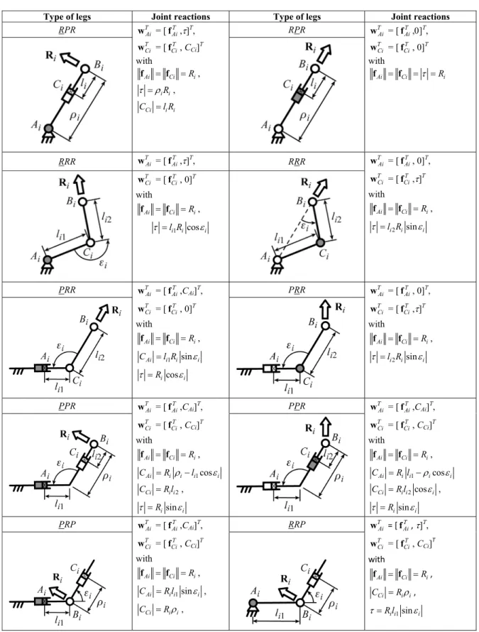
Table 2. Norm of the reaction effort inside of the leg joints of planar parallel robots.
Type of legs Joint reactions Type of legs Joint reactions
RPR T Ai w = [ T Ai f ,]T, T Ci w = [ T Ci f , CCi]T with Ai Ci Ri f f , i iR , Ci i i C l R RPR T Ai w = [ T Ai f ,]T, T Ci w = [ T Ci f , 0]T with Ai Ci Ri f f RRR w = [TAi f ,AiT ]T, RRR w = [TAi f , 0]TAi T, T Ci w = [ T Ci f ,]T with Ai Ci Ri f f , 2 sin i i i l R T Ci w = [ T Ci f , 0]T with Ai Ci Ri f f , 1 cos i i i l R PRR T Ai w = [ T Ai f ,CAi]T, T Ci w = [ T Ci f , 0]T with Ai Ci Ri f f , 1 sin Ai i i i C l R cos i i R PRR T Ai w = [ T Ai f , 0]T, T Ci w = [ T Ci f ,]T with Ai Ci Ri f f , 2 sin i i i l R PPR T Ai w = [ T Ai f ,CAi]T, T Ci w = [ T Ci f , CCi]T with Ai Ci Ri f f , 1cos Ai i i i i C R l 2 Ci i i C R l , sin i i R PPR T Ai w = [ T Ai f ,CAi]T, T Ci w = [ T Ci f , CCi]T with Ai Ci Ri f f , 1 cos Ai i i i i C R l 2cos Ci i i i C R l , sin i i R PRP T Ai w = [ T Ai f ,CAi]T, T Ci w = [ T Ci f , CCi]T with Ai Ci Ri f f , 1sin Ai i i i C R l , Ci i i C R , RRP T Ai w = [ T Ai f ,]T, T Ci w = [ T Ci f , CCi]T with Ai Ci Ri f f , Ci i i C R , 1sin i i i R l
Fig. 4. Kinematic chain of the planar five-bar robot. - a = 0.1375 m
In the following of the paper, it is considered that the leg 1 is composed of the segments AB and BP and that leg 2 is composed of segments ED and DP. The active joints are located at points A and E.For five-bar mechanisms, it can be shown that the matrix
AT of (2) is equal to [1]: 1 2 1 2 cos cos sin sin T 1 2 A r r . (33)
Moreover, disconnecting leg 1 (2, resp.) from the end-effector, for a fixed position of the actuator 2 (1, resp.), the direction v1 (v2,
resp.) of the translational velocity vector of the end-point of leg 2 (1, resp.) is orthogonal to the direction of the segment DP (BP, resp.) (Fig. 4). Therefore,
2 2 sin cos 1 v . (34) As a result,
1 1 1 2 1 1 1 2cos cos sin
cos sin cos
T T 1 1 1 1 2 2 2 2 r v r v r v r v . (35)
where is the angle between segments BP and DP (Fig. 4). Please note that:
- is denoted as the transmission angle of the robot [9]; - fixing angle is equivalent to fixing the shape of the
triangle BPD and the robot can be shown as a 1-DOF planar four-bar mechanism (Fig. 5).
Taking only into account the each revolute joint can admit a maximal force Radm, and as for such mechanisms no moments are
applied on the controlled point, the only condition for non breakdown of the mechanism under a force f applied at P is given by f Radmcos. Knowing f and Radm, this remains to fixing the
maximal value max of .
For a fixed angle max, four possible values of are possible
(Fig. 5):
(a) assembly mode 1, 1
1 sin cos
(b) assembly mode 2, 2 1
(c) assembly mode 3, 3 1
(d) assembly mode 4, 4 1
Fig. 5. The four equivalent 4-bars mechanisms, for a fixed value of max.
1
1 sin cos max
,
2 1
, 3 , 1 4 . (36) 1 Therefore, four four-bar mechanisms can be studied, depending on the assembly mode of the five-bar robot (Fig. 5). Therefore, the constant pressure angle loci, and as a result, the constant joint reaction loci, can be found algebraically by studying the displacement of points P of the four-bar mechanisms. These borders are portions of sextic curves [1].
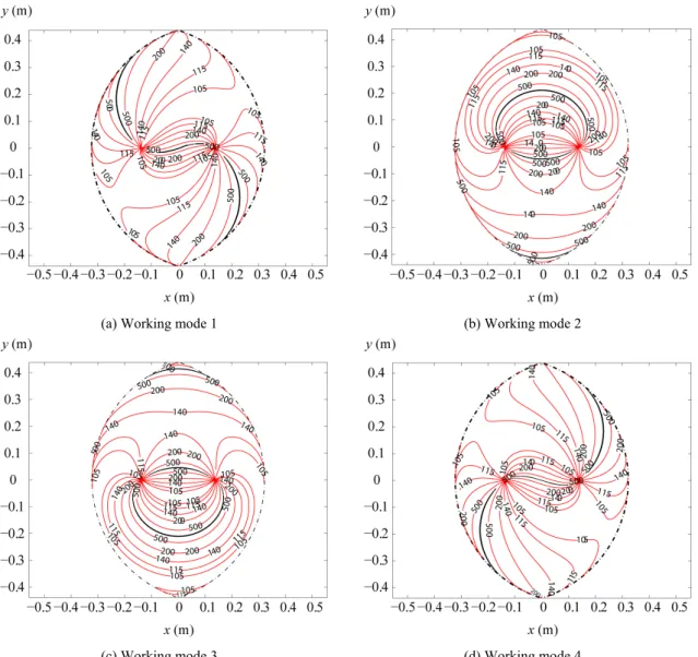
The variations of the joint reaction within the workspace of the DexTAR robot, on which is applied a force equal to 100 N, are presented in Fig. 6 for the four working modes of the robot. On this picture, the dotted black lines correspond to the Type 1 singularities and the full black lines to the Type 2 singularities [4], i.e. the maximal workspace boundaries. It can be shown that, the closer the robot from Type 2 singular configurations, the higher the joint reactions.
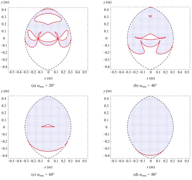
In [25], it is shown that the DexTAR is able to pass through Type 1 singularities [4]. For one given assembly mode, a position of the end-effector is able to be attained by two working modes. Taking this result into account, the borders of the force workspace
for a given assembly mode are computed. As previously, these borders can also be found algebraically, by studying the displacement of points P of the four-bar mechanisms. For one given assembly mode, a point of the sextic curves will belong to the border of the force workspace if the pressure angle of the mechanism at this end-effector position is always superior or equal to max for any of the working modes. If not, this point can
be reached by at least one of the working modes, i.e. it is not a workspace boundary. Some examples of the force workspace, for several values of , are presented in Fig. 7. Obviously, the smaller max, the smaller the workspace. When max is large, the
(a) Working mode 1 (b) Working mode 2
(c) Working mode 3 (d) Working mode 4
Fig. 6. Variation of the robot joint reaction (in Newton) within the workspace for f = 100 N.
workspace has only one aspect. For max small, several aspects
will appear.
B. The 3-RPR robot
The PAMINSA (Fig. 8) is a parallel manipulator with 4 DOF (Schoenflies motions) of which translation along the vertical axis is decoupled from the displacement in the horizontal plane. When the vertical translational motion is locked up, the PAMINSA is fully equivalent to a 3-RPR manipulator (Fig. 8b) with equilateral platform and base triangles, of which circumcircles have the following radii:
- for the base, Rb = 0.35 m
- for the platform, Rp = 0.1 m
For 3-RPR robots, it can be shown that the matrix AT of (2)
expressed at point Bi is equal to [26]:
1 2 3 T C C C 1 2 3 w1 w2 w3 r r r A s s s . (37)
with T sin cos
i qi qi r and 1 0 C , 2 3 sin cos T p C R r , 2
3 sin / 3 3 cos / 3 T p C R r , if B3 i = B1 (38a)
1 sin 3 cos T p C R r , 1 C2 , 0(a) max = 20° (b) max = 40°
(c) max = 60° (d) max = 80°
(a) PAMINSA prototype
(b) equivalent model of the planar displacements Fig. 8. Kinematics of the PAMINSA.
3 sin 2 / 3 3 cos 2 / 3 T p C R r , if B3 i = B2 (38b)
1 sin 4 / 3 3 cos 4 / 3 T p C R r , 1
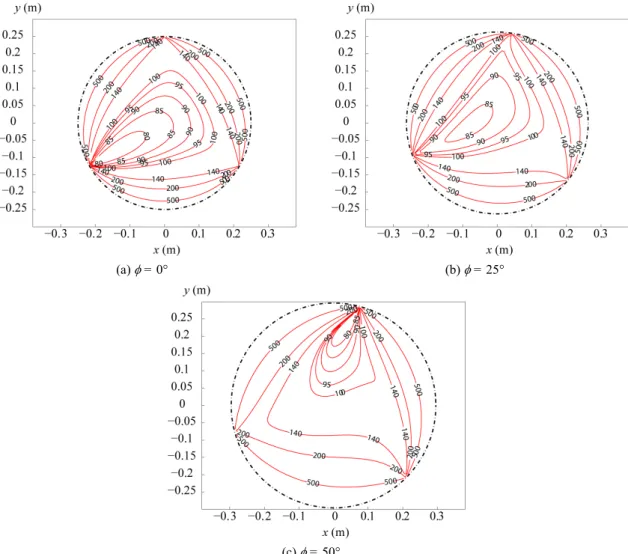
2 sin / 3 3 cos / 3 T p C R r , 2 C3 , if B0 i = B3 (38c) For this mechanism, the way to compute the pressure angle and the distance between the observed joint and the platform instantaneous centre of rotation is explained in [7].The variations of the joint reaction at point B1 within the
workspace for several platform orientations are presented in Fig. 9 for f = 100 N and C = 5 Nm. The dotted lines correspond to the Type 2 singularities that appear if [26]:
- for a given orientation of the platform, the point P is located on a circle C() centred in O, of radius equal to
2 2 2 cos
b p b p
R R R R
- for orientations cos (1 / )
p b
R R
, the robot is in
singular configuration for any position of P.
It can be observed that, the closer from Type 2 singularities, the higher the joint reaction. Moreover, the lowest values of the joint reactions appear in the centre of the workspace.
Let us analyze the force workspace of the robot. On the contrary of the DexTAR for which the obtained expressions are symbolic, and the force workspace boundaries can be obtained algebraically, for this robot, a numerical method has to be used. The method consists in discretising the workspace using polar coordinates (r, ). For one given angle , the algorithm tests for all rising values of r that the manipulator can support the applied wrench (see tables 1 and 2). In the case where the manipulator cannot support the applied wrench, the boundary of the force workspace is defined by the previous computational point.
In the remainder of this example, we take only into account the maximal admissible value Radm of the reactions of the revolute
joints located at Bi. It is applied on the platform a force of norm f
= 100 N, and a moment of norm C = 5 Nm. The shape of the force workspace, for one given assembly mode and for several values of Rmax and platform orientation is shown in Fig. 10.
It can be observed that, the greater the value of , i.e. the closer from the orientation for which the robot is in singular configuration for any position of the platform centre, the smaller the workspace.
V. Conclusions
This paper extends the previous works on the quality of the effort transmission in iso-static planar closed-loop mechanisms. The traditional transmission indices only show the ratio between input and output powers but they don’t show an unacceptable high increase of the reactions in the passive joints. In this study, it is disclosed that the increase of reactions in passive joints depends not only on the transmission angle but also the position of the instantaneous centre of rotation of the platform. This is the first time that such a kinetostatic property is rigorously formulated and clearly demonstrated. The obtained results allow expanding the knowledge about the effort transmission quality. They are complementary conditions to the traditional transmission indices and allow avoiding a breakdown close to the singularity. In this aim, the boundaries for the admissible values of the transmission angle and of the distance to the instantaneous centre of rotation are computed. The Dextar and the 3-RPR robot have been studied as illustrative examples. The effort transmission in these manipulators has been studied as well as their reachable workspaces taking into account the limitation of the efforts in passive joints.
Finally, it should be noted that in this paper, the disclosed properties have been only devoted to the study of planar parallel mechanisms. It is quite possible that such a concise and accurate criterion can be also obtained for spatial case. In our future work we will try to extend this approach to spatial parallel mechanisms, but it is a real challenge.
References
[1] Merlet, J.P. (2006) Parallel robots. Springer, 2nd Ed.
[2] Bonev, I.A., Zlatanov, D. and Gosselin, C.M. (2003). Singularity analysis of 3-DOF planar parallel mechanisms via screw theory. ASME Journal of Mechanical Design, 125(3):573–581.
[3] Daniali, M.H.R, Zsombor-Murray, P.J. and Angeles, J. (1995) Singularity analysis of planar parallel manipulators. Mechanism and Machine Theory, 30(5), 665–678.
[4] Gosselin, C.M. and Angeles, J. (1990). Singularity analysis of closed-loop kinematic chains. IEEE Transactions on Robotics and Automatics, 6(3): 281–290. [5] Zlatanov, D., Bonev, I.A. and Gosselin, C. M. (2002).
Constraint singularities of parallel mechanisms. IEEE International Conference on Robotics and Automation, Washington, D.C., USA, May 11-15.
[6] Sutherland, G., and Roth, B. (1973) A transmission index for spatial mechanisms. ASME Journal of Engineering for Industry. 589–597.
[7] Arakelian, V., Briot, S., Glazunov, V. (2008). Increase of singularity-free zones in the workspace of parallel manipulators using mechanisms of variable structure. Mechanism and Machine Theory, 43(9):1129–1140. [8] Alba-Gomez, O., Wenger, P. and Pamanes, A. (2005). A
Consistent kinetostatic indices for planar 3-DOF parallel manipulators, application to the optimal kinematic inversion. Proceedings of the ASME 2005 IDETC/CIE Conference, September 24-28, Long Beach, California. [9] Balli, S. and Chand, S. (2002). Transmission angle in
mechanisms. Mechanism and Machine Theory, 37: 175-195.
[10] Angeles, J. and López-Cajún, C., (1991) Optimization of cam mechanisms. Kluwer Academic Publishers B. V., Dordrecht
(a) = 0° (b) = 25°
(c) = 50°
Fig. 9. Variations of the joint reaction (in Newton) at point B1 within the workspace for several platform orientations , for f = 100 N
and C = 5 Nm.
(a) = 0°, Rmax = 200 N (b) = 0°, Rmax = 110 N
(c) = 25°, Rmax = 200 N (d) = 25°, Rmax = 110 N
(e) = 50°, Rmax = 200 N (f) = 50°, Rmax = 110 N
[11] Chen, C. and Angeles, J. (2007). Generalized transmission index and transmission quality for spatial linkages. Mechanism and Machine Theory, 42(9), 1225-1237. [12] Gosselin, C.M. and Angeles, J. (1991). A global
performance index for the kinematic optimization of robotic manipulators, Journal of Mechanical Design, 113(3):220–226.
[13] Merlet, J.-P. (2006). Jacobian, manipulability, condition Number, and accuracy of parallel robots, ASME Journal of Mechanical Design, 128(1): 199–206.
[14] Rakotomanga, N., Chablat, D., and Caro, S. (2008). Kinetostatic performance of a planar parallel mechanism with variable actuation. 11th International Symposium on Advances in Robot Kinematics, Kluwer Academic Publishers, Batz-sur-mer, France, June.
[15] Ranganath, R., Nair, P.S., Mruthyunjaya, T.S. and Ghosal, A. (2004). A force–torque sensor based on a Stewart Platform in a near-singular configuration. Mechanism and Machine Theory 39(9): 971–998.
[16] Stocco, L., Salcudean, S., and Sassani, F. (1998) Fast constrained global minimax optimization of robot parameters. Robotica, 16:595–605.
[17] Hayward, V., Choksi, J., Lanvin, G., and Ramstein, C. (1994). Design and multi-objective optimization of a linkage for a haptic interface. Advances in Robot Kinematics: 352–359.
[18] Frisoli, A., Prisco, M., Salsedo, F., and Bergamasco, M. (1999) A two degrees-of-freedom planar haptic interface with high kinematic isotropy. Proceedings of the 8th IEEE International Workshop on Robot and Human Interaction (RO-MAN'99): 297–302.
[19] Liu, X.-J., Wu, C., and Wang, J. (2012) A New approach for singularity analysis and closeness measurement to singularities of parallel manipulators. ASME Journal of Mechanisms and Robotics, 4.
[20] Takeda, Y. and Funabachi, H. (1995). Motion transmissibility of in-parallel actuated manipulators. Transactions JSME series C, 38(4): 749–755.
[21] Takeda, Y. and Funabachi, H. (1996). Kinematic and static characteristics of in-parallel actuated manipulators at singular points and in their neighborhood. Transactions JSME series C, 39(1): 85–93.
[22] Hubert, J. and Merlet, J.-P. (2009). Static of parallel manipulators and closeness to singularity. Journal of Mechanisms and Robotics, 1(1).
[23] Briot, S., Pashkevich, A. and Chablat, D. (2010). Optimal technology-oriented design of parallel robots for high-speed machining applications. Proceedings of the 2010 IEEE International Conference on Robotics and Automation (ICRA 2010), May 3-8, Anchorage, Alaska, USA.
[24] Terminology for the mechanism and machine science (2003), Mechanism and Machine Theory, 38.
[25] Campos, L., Bourbonnais, F., Bonev, I.A. and Bigras, P. (2010). Development of a five-bar parallel robot with large workspace. Proceedings of the International Design Engineering Technical Conferences & Computers and Information in Engineering Conference IDETC/CIE, August 15-18, Montréal, Québec, Canada.
[26] Briot, S., Arakelian, V. and Guégan, S. (2008). Design and prototyping of a partially decoupled 4-DOF 3T1R parallel manipulator with high-load carrying capacity. Journal of Mechanical Design, 130(12).
[27] Chablat, D., Wenger, P., and Angeles, J. (1998). The isoconditioning loci of a class of closed-chain manipulators. Proceedings of the IEEE International Conference on Robotics and Automation, May, pp. 1970– 1976.