HAL Id: hal-00796353
https://hal.archives-ouvertes.fr/hal-00796353
Submitted on 4 Mar 2013
HAL is a multi-disciplinary open access
archive for the deposit and dissemination of
sci-entific research documents, whether they are
pub-lished or not. The documents may come from
teaching and research institutions in France or
abroad, or from public or private research centers.
L’archive ouverte pluridisciplinaire HAL, est
destinée au dépôt et à la diffusion de documents
scientifiques de niveau recherche, publiés ou non,
émanant des établissements d’enseignement et de
recherche français ou étrangers, des laboratoires
publics ou privés.
Probabilistic lifetime assessment of RC structures under
coupled corrosion-fatigue deterioration processes
Emilio Bastidas-Arteaga, Philippe Bressolette, Alaa Chateauneuf, Mauricio
Sánchez-Silva
To cite this version:
Emilio Bastidas-Arteaga, Philippe Bressolette, Alaa Chateauneuf, Mauricio Sánchez-Silva.
Proba-bilistic lifetime assessment of RC structures under coupled corrosion-fatigue deterioration processes.
Structural Safety, Elsevier, 2009, 31, pp.84-96. �10.1016/j.strusafe.2008.04.001�. �hal-00796353�
Probabilistic lifetime assessment of RC structures under coupled
corrosion-fatigue deterioration processes
Emilio Bastidas-Arteaga
a,b, Philippe Bressolette
b, Alaa Chateauneuf
b,
Mauricio S´
anchez-Silva
aa
Department of Civil and Environmental Engineering. Universidad de los Andes, Carrera 1 N. 18A-70 Edificio Mario
Laserna. Bogot´a, Colombia
b
Laboratorie de G´enie Civil - Universit´e Blaise Pascal - BP 206-63174 Aubi`ere cedex, France
Abstract
Structural deterioration is becoming a major problem when considering long term performance of infrastructures. The existence of a corrosive environment, cyclic loading and concrete cracking cause structural strength degradation. The interaction of these conditions can only be taken into account when modeling the coupled action. In this paper, a new model to assess lifetime of RC structures subject to corrosion-fatigue deterioration processes, is proposed. Separately, corrosion leads to cross section reduction while fatigue induces the nucleation and the propagation of cracks in steel bars. When considered together, pitting corrosion nucleates the crack while environmental factors affect the kinematics of crack propagation. The model is applied to the reliability analysis of bridge girders located in different chloride-contaminated environments. Overall results show that the coupled effect of corrosion-fatigue on RC structures affects strongly its performance leading to large reduction in the expected lifetime.
Key words: corrosion-fatigue, chloride ingress, cyclic load, lifetime assessment, reinforced concrete, reliability.
1. Introduction
Long-term performance of infrastructure systems is dominated by structural deterioration. Structural deterioration is loss of capacity due to physical, chemical, mechanical or biological actions. Since a corrosive environment and cyclic loading are two of the main causes of reinforced concrete (RC) deterioration, a significant amount of research has been devoted to these two specific damage mechanisms [1] [2] [3]. Corrosion is the most common form of steel deterioration and consists in material disintegration as a result of chemical or electrochemical action. Most metals corrode on contact with water (or moisture in the air), acids, bases, salts, and other solid and liquid chemicals. Metals will also corrode when exposed to gaseous materials like acid vapors, formaldehyde gas, ammonia gas, and sulfur containing gases [3]. Depending upon the case, corrosion can be concentrated locally to form a pit, or it can extend across a wide area to produce general wastage. On the other hand, fatigue is the damage of a material resulting from repeatedly stress applications (e.g. cyclic loading). Fatigue is conditioned by factors such as high temperature, i.e. creep-fatigue, and the presence of aggressive environments, i.e. corrosion-fatigue [1] [2].
The damage to RC structures resulting from the corrosion of reinforcing is exhibited in the form of steel cross section reduction, loss of bond between concrete and steel, cracking, and spalling of concrete cover [4] [5]. The corrosion of steel reinforcement has been usually associated to chloride ingress and carbonation [4]; however, recent studies have shown that other deterioration processes like biodeterioration might contribute significantly to this process [6]. In RC structures, the coupled effect of corrosion and fatigue has not been studied in as much detail as their separated effects. Coupled corrosion-fatigue deterioration results from the combined action of cycling stresses in corrosive environments. Localized corrosion leading to pitting may
provide sites for fatigue crack initiation. Corrosive agents (e.g., seawater) increase the fatigue crack growth rate [7], whereas the morphology of metals/alloys at micro-level governs the pit nucleation sites [8]. Under these conditions, the formation and growth of pits is influenced by both a corrosive environment and cyclic loads and become a coupled damage mechanism.
Examples of structures that experience this type of damage are bridges, chimneys, towers and offshore structures situated close to the sea or exposed to the application of de-icing salts. The effects of gradually accumulating corrosion on the low cycle fatigue of reinforcing steel have been recorded experimentally by Apostolopoulos et al. [9] showing that corrosion implies an appreciable reduction in the ductility, the strength and the number of cycles to failure.
Large research efforts have been made to predict the corrosion-fatigue life of structural members consti-tuted by aluminum, titanium and steel alloys. Goswami and Hoeppner [10] proposed a seven-stage conceptual model in which the electrochemical effects in pit formation and the role of pitting in fatigue crack nucle-ation were considered. Other research studies focused on particular stages of the process. For instance, a transition model from pit to crack based in two criteria: stress intensity factor and the competition between pit growth and crack growth, was proposed by Kondo [11], and further discussed by Chen et al. [12]. In order to take into consideration the entire progressive damage process and the uncertainties in each stage, Shi and Mahadevan [13] proposed a mechanics-based probabilistic model for pitting corrosion fatigue life prediction of aluminum alloys.
The objective of this paper is to develop a probabilistic lifetime prediction model for RC structures under the coupled effect of corrosion and fatigue. The model assesses the total corrosion-fatigue life as the sum of three critical stages: (1) corrosion initiation and pit nucleation; (2) pit-to-crack transition, and (3) crack growth. The first considers the time from the end of construction until the generation of a pit. The length of this stage is estimated by considering Frick’s diffusion law and electrochemical principles. The second stage includes the pit growth until crack nucleation. In this stage the interaction between electrochemical and mechanical processes is taken into account. The latter stage covers the time of crack growth until it reaches a critical crack size. The critical crack size is defined as the crack size at which the RC member reaches a limit state of resistance.
The model proposed is exposed in section 2. Section 3 presents a discussion about time-dependent relia-bility analysis. Finally, an application to bridge girders is exposed in section 4.
2. Coupled corrosion-fatigue model
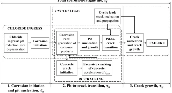
The corrosion-fatigue damage process in RC structures is conceptually depicted in Figure 1. The process takes into account the interaction between: (1) chloride ingress, (2) RC cracking and (3) cyclic load. Chloride ingress leads to steel depassivation, and takes part in the kinematics of the corrosion process. Besides, corrosion as a result of chloride ingress induces a high localized corrosion (i.e., pitting corrosion) leading to reinforcing steel crack nucleation [3]. Concrete cracking generated by the accumulation of corrosion products in the steel/concrete interface plays an important role in the steel corrosion rate. Its importance depends of both the width of the crack in the concrete and the aggressiveness of the environment. On the other hand, cyclic loading is important in the transition from pit to crack and crack growth.
The corrosion-fatigue deterioration process is basically divided in two stages: (1) pit formation and growth; and (2) fatigue crack growth. Pit formation and growth involves electrochemical processes depending pre-dominantly on environmental factors. Crack growth is estimated in terms of Linear Elastic Fracture Mechan-ics (LEFM) and depends mostly upon both cyclic loads and material properties. Goswami and Hoeppner [10] proposed to separate conceptually the corrosion-fatigue life into the following stages: (1) electrochemical stage and pit nucleation, (2) pit growth, (3) competitive mechanisms between pit growth and fatigue crack nucleation, (4) chemically, ”short” crack growth, (5) transition from ”short crack” to ”long crack”, (6) long crack growth, and (7) corrosion fatigue crack growth until instability. However, assuming initial immunity of RC structures and the fact that some of these stages proposed by Goswami and Hoeppner are transitional stages, the total corrosion-fatigue life, τT, will be divided in the following stages (Figure 1):
(i) corrosion initiation and pit nucleation, τcp, (ii) pit-to-crack transition, τpt, and
2.1. Corrosion initiation and pit nucleation This stage is divided into two sub-stages: (i) time to corrosion initiation, τini, and (ii) time to pit nucleation, τpn.
The first describes the time from the end of construction until the depassivation of the corrosion protective layer of reinforcing steel, and subsequently, corrosion initiation. For RC structures, the length of this stage depends mainly upon the concrete characteristics and the thickness of the cover. It is calculated by using the Frick’s second law under the assumption that concrete is an homogenous and isotropic material [14]:
∂C
∂τ = Dcl
∂2C
∂x2 (1)
where C is the chloride ion concentration, Dcl is the chloride diffusion coefficient in concrete, τ is the time and x is depth in the diffusion direction. If the following initial conditions are defined: (1) at time τ = 0, the chloride concentration is zero; (2) the chloride concentration on the surface is constant. The solution to eq. 1 leads to the chloride ion concentration C(x, τ ) at depth x after time τ :
C(x, τ ) = Cs 1 − erf ✓ x 2√Dclτ ◆$ (2)
where Cs is the surface chloride concentration and erf() is the error function. The threshold concentration
Cth is defined as the chloride concentration for which the rust passive layer of steel is destroyed and the
corrosion begins. When C(x, τ ) is equal to Cth and the depth x is equal to the bar cover c, i.e. x = c, the
time to corrosion initiation, τini, becomes: τini= c2 4Dcl erf−1 ✓ 1 −CCth s ◆$−2 (3) Pit nucleation is the result of an electrochemical processes induced by corrosion. Computing time to
pit nucleation, τpn, is a non-trivial task because its value depends on several environmental, material and
loading factors whose interaction is not well understood yet. The pit depth at time τ , p(τ ) (Figure 2b), can be calculated as [3]:
p(τ ) = 0.0116α Z
icorr(τ )dτ (4)
where p(τ ) is given in mm, α is the ratio between pitting and uniform corrosion depths, and icorr(τ ) is the
time-variant corrosion rate which is given in µA/cm2. Time to pit nucleation is estimated by defining a
threshold, p0, for the pit depth, p(τ ). For example, according to Harlow and Wei [15] this value is p(τpn) =
p0 =1.98×10⁻⁶m. During a brief time period after steel depassivation, i.e. τini+ 1yr≥ τ > τini, it is
reasonable to assume that icorr(τ ) remains constant (i.e. icorr(τ ) = iini) and is equal to [16]: iini= 37.8(1 − wc)
−1.64
c (5)
where wc is the water-cement ratio and c is given in mm. Consequently, by making p(τpn) = p0 in eq. 4,
substituting eq. 5 in eq. 4 and by integrating, the time to pit nucleation, τpn, can be written: τpn=
2.281cp0
α (1 − wc)
1.64 (6)
Equation 6 gives a simple relationship to estimate τpnbased on electrochemical principles. Other proposals
to obtain τpncan be found in the literature [13], however, this discussion is beyond the scope of this paper.
2.2. Pit-to-crack transition
The time of transition from pit to crack, τpt, is defined as the time at which the maximum pit depth
reaches a critical value leading to crack nucleation. Crack nucleation depends on the competition between the processes of pit and crack growth. To estimate this transition period, two criteria can be taken into account [11] [12]:
(i) Rate competition criterion: the transition takes part when the crack growth rate, da/dτ , exceeds the pit growth rate, dp/dτ , as illustrated in Figure 2a.
(ii) Fatigue threshold criterion: the transition occurs when the stress intensity factor of the equivalent
surface crack growth for the pit, ∆Keq, reaches the threshold stress intensity factor for the fatigue
crack growth, ∆Ktr.
In this study, the fatigue threshold criterion was not taken into consideration because experimental observations indicate that this criterion is not appropriate to estimate fatigue crack nucleation at low loading frequencies [12]. Therefore, the rate competition criterion where pit growth rate is described by electrochemical mechanisms and fatigue crack growth rate is estimated in terms of LEFM will be discussed in the following sections. This discussion will focus on:
(i) Pit growth rate
(ii) Fatigue crack growth rate
(iii) Computation of pit-to-crack transition 2.2.1. Pit growth rate
After pit nucleation and as a result of a localized galvanic corrosion, pit growth can be estimated in terms of a change in the volumetric rate by using the Faraday’s law [11] [15]:
dV
dτ =
M icorr
nF ρ (7)
where M is the molecular weight of iron, (i.e. M = 55.85 g/mol), icorr is the corrosion rate, n is the valence
of iron, (i.e. n = 2), F is the Faraday’s constant, (i.e. F = 96500 C/mol), and ρ is the density of iron, (i.e.
ρ = 8000 kg/m3). Corrosion rate is the effective galvanic current between the particles and the steel matrix.
The relationship between corrosion rate and temperature is taken into account by using the Arrhenius equation: icorr= ip0exp ✓ −∆H RT ◆ (8)
where ip0 is the pitting current coefficient, ∆H is the activation enthalpy, R is the universal gas constant
(R = 8.314/mol K), and T is the absolute temperature. It is clear, from eq. 8, that the corrosion rate increases when temperature is raised. Nevertheless, given the complexity of the corrosion process in RC,
the relationship between icorr and T is not simple [17]. For instance, it has been found that the corrosion
kinetics of different RC structures under conditions of constant temperature can vary widely [17]. This variability results from the interaction between temperature and other factors such as conductivity and relative humidity. In addition, corrosion rate in RC is a function of environmental aggressiveness. Thus, the corrosion rate becomes a time-variant function depending mostly upon: concrete pH, oxygen, water and chlorides availability. In this context, Bastidas-Arteaga et al. [18] proposed a time-variant corrosion
rate function, icorr(τ ), which takes into account environmental hostility. This function is based on a fuzzy
inference system under the following assumptions:
(i) during the period corresponding to the initial corrosion age, the initial corrosion rate function, iini(τ ) is estimated as [16]: iini(τ ) = 2 6 4 37.8(1 − wc)−1.64
c if τini+ 1yr ≥ τ > τini
32.13(1 − wc)−1.64 c (τ − τini) −0.3 if τ > τ ini+ 1yr 3 7 5; (9)
(ii) during the period corresponding to the maximum corrosion age, icorr leads to a maximum corrosion
rate, imax. The value of imax depends principally on the availability of water, oxygen and salts at the corrosion cell as a result of severe concrete cracking.
If the membership function for the initial corrosion age is µini(τ ) and for the maximum corrosion age
is µmax(τ ), the time-variant corrosion rate considering concrete cracking and environmental aggressiveness
takes the form: icorr(τ ) =
µini(τ )iini(τ ) + µmax(τ )imax µini(τ ) + µmax(τ )
(10) Figure 2b depicts the time-variant corrosion rate functions. It is observed that the initial corrosion rate function (i.e. dotted line) decreases after τini+ 1 yr. This is caused by the formation of rust products on the steel surface that reduce the diffusion of iron ions away from the steel surface. Moreover, the accumulation of corrosion products reduces the area ratio between the anode and the cathode [16]. The time-variant corrosion
rate (i.e. continuous line) follows the initial corrosion rate function until the time for several concrete
cracking. After the time of severe cracking, τsc, there is a transition towards the maximum corrosion rate.
The advantage of this fuzzy approach is that the corrosion rate can be estimated based on local conditions, experts’ knowledge and empirical models or observations. For example, for a given site, an expert can define the shape of the membership functions or the value of the maximum corrosion rate taking into account its knowledge about concrete quality, material properties, environmental hostility, RC behavior in similar conditions etc. Finally, it is important to clarify that the function can be permanently updated based on field measurements and experimental data.
Pit formation and shape are random phenomena which depend mainly on material properties, fabrication processes and electrochemical factors [10]. Currently this dependence is not well understood. Some authors assume that pit growth follows the shape of a hemisphere or a prolate spheroid [15] [11]. For simplicity, a spherical shape of the pit is assumed herein (Figure 2b) and its radius, p(τ ), can be estimated from eq. 4. Then, the volumetric rate of pit growth (eq. 7) can be directly rewritten in terms of pit growth rate by deriving eq. 4 with respect to time:
dp
dτ = 0.0116αicorr(τ ) (11)
2.2.2. Fatigue crack growth rate
The fatigue crack growth rate is estimated by means of the Paris-Erdogan law: da
dN = Cp(∆K)
m (12)
where a is the crack size, N is the number of cycles, ∆K is the alternating stress intensity factor, and Cpand
m are material constants. It is know that there is a strong correlation between Cpand m, and their values
are highly depending on the environmental aggressiveness. For RC structures, Salah el Din and Lovegrove
[19] reported experimental values for Cp and m corresponding to medium and long crack growth stages,
leading to: da dN = 2 4 3.83 × 10⁻²⁹(∆K)20.863 if ∆K ≤ 9 MPa√m 3.16 × 10⁻¹²(∆K)3.143 otherwise 3 5 (13)
and the stress intensity factor, ∆K, is computed as:
∆K(a) = ∆σY (a/d0)√πa (14)
where ∆σ is the stress range, i.e. ∆σ = σmax− σmin, d0is the initial diameter of the bar and Y (a/d0) is a dimensionless geometry notched specimen function, which can be approximated by [20]:
Y (a/d0) = 1.121 − 3.08(a/d0
) + 7.344(a/d0)2− 10.244(a/d0)3+ 5.85(a/d0)4 [1 − 2(a/d0)2]3/2
(15) The dotted line in Figure 2a follows the shape of the fatigue crack growth rate as function of time, which starts growing after corrosion initiation and pit nucleation.
2.2.3. Computation of pit-to-crack transition
In order to find the time for pit-to-crack transition, τpt, an equivalent stress intensity factor for the pit,
∆Kpit must be estimated. ∆Kpit is found by substituting a in eq. 14 by the pit depth p(τ ) (eq. 4):
∆Kpit(τ ) = ∆σY (p(τ )/d0)pπp(τ) (16)
Then, the equivalent crack growth rate becomes: da
dτ = Cp[∆Kpit(τ )] m
f (17)
where f is the frequency of the cyclic load. Therefore, the time of pit-to-crack transition is obtained by
equating the pit growth rate (eq. 11) with the equivalent crack growth rate (eq. 17), and solving for τpt in:
0.0116αicorr(τpt) = Cp(∆Kpit(τpt))mf (18)
In order to calculate τpt, eq. 18 must be solved numerically. Figure 2a illustrates the graphical solution
2.3. Crack growth
Crack growth modeling is concerned with the time from the crack initiation until the crack size has reached a value that defines the failure of the cross section. The size of the initial crack on the steel reinforcement, a0, is estimated as the pit depth when the transition from pit to crack is reached, i.e. a0= p(τpt) (eq. 4).
The size of the critical crack, ac, is defined as the crack size at which the RC member reaches a limit state
of resistance (e.g. bending capacity). This time is obtained as:
τcg= 1 f 2 6 6 4 Z a1 a0 da 3.83 × 10⁻²⁹(∆K)20.863 + Z ac a1 da 3.16 × 10⁻¹²(∆K)3.143 if a0< a1 Z ac a0 da 3.16 × 10⁻¹²(∆K)3.143 otherwise 3 7 7 5 (19)
where a1is the crack size at which the crack growth rate changes from medium to long crack growth. The
transition between medium and long crack growth occurs when the crack size reaches a threshold stress intensity factor -i.e. ∆K(a1) = 9 MPa√m [19].
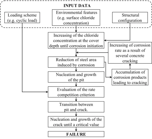
The flowchart that summarizes the entire procedure is presented in Figure 3. The corrosion initiation process depends upon both environmental features and structural configuration. After corrosion initiation, the accumulation of corrosion products in the concrete/steel interface increases the corrosion rate as a result of concrete cracking. By considering the interaction between pit growth and cyclic load, the rate competition criterion is evaluated, and consequently, the time of pit-to-crack transition is assessed. Finally, once crack growth has become the preponderating process, the crack growth induces failure in the cross section.
This model allows the evaluation of the total structural lifetime including: corrosion initiation, pit-to-crack transition and pit-to-crack propagation. Its robustness lies in the implicit integration of various parameters and processes affecting the RC lifetime, which is very convenient for reliability analysis.
3. Time-dependent reliability analysis
The cumulative distribution function (CDF) of the total corrosion-fatigue life, FτT(τ ), is defined as [21]:
FτT(τ ) = Pr{τT ≤ τ} =
Z
τcp+τpt+τcg≤τ
f (x) dx (20)
where x is the vector of the random variables taken into account and f (x) is the joint probability density function of x. If structural failure is achieved when the crack size reaches a critical value inducing failure of the cross section, the limit state function becomes:
g (x,τ ) = ac(x) − aτ(x,τ ) (21)
where aτ(x,τ ) is the crack size at time τ and ac(x) is the critical crack size defined in terms of a limit state of resistance. For example, if the limit state of bending capacity is chosen, since the crack growth induces a reduction in the bending capacity of the structural member, the ultimate bending capacity is reached when ac is achieved. By taking into account eq. 21, the failure probability, pf, can be estimated as:
pf= Z
g(x,τ )≤0
f (x) dx (22)
Corrosion-fatigue deterioration process is a time-dependent problem where conditional probabilities are involved. Given the complexity of the problem, closed form solutions for both the CDF of the total corrosion-fatigue lifetime and the failure probability are difficult to obtain. To solve this problem, it is necessary to use Monte-Carlo simulations or analytical approximations such as FORM/SORM.
4. Application to bridge girder
This section presents an illustrative example describing the coupled effect of corrosion-fatigue of a simply supported RC bridge girder subject to cyclic loading. The span of the girder is 10 m with the geometrical characteristics of the cross section and the steel reinforcement shown in Figure 4. The girder has been designed according to EUROCODE 2 [22]. Besides the dead load, a truck wheel load is applied on the
girder. The design load, Pk, corresponds to a wheel load located in the center of the span. Table 1 presents
In order to study the implications of the traffic frequency, f , the values of 50, 500, 1000 and 2000 cycles/day are considered. It is important to stress that these frequencies are in the range defined by the EUROCODE 1 for heavy trucks [22]. The effect of environmental hostility on structural reliability, was considered by taken into consideration four levels of aggressiveness (Table 2). Each level is characterized by: (1) a chloride
surface concentration, Cs, (2) a maximum expected value of the corrosion rate, imax, and (3) a concrete
cover, c. The chloride surface concentration is treated as a random variable for which the mean depends largely on proximity to sea and is computed based on the work of McGee [23]. The maximum expected values of the corrosion rate are based on the EN206 [24]. The cover is defined according to EUROCODE 2 [22]. Table 2 summarizes the characteristics of each level of environmental aggressiveness.
The basic considerations and assumptions of the study are:
– Section confinement is taken into account by using the Kent and Park model [25] and stress-strain rela-tionship for steel follows an elasto-plastic model.
– The elasticity modulus and the tensile strength of concrete are given in terms of the compression strength according to EUROCODE 2 [22].
– A limit crack width of 0.5 mm is used as a threshold for severe concrete cracking, τsc.
– The water/cement ratio is calculated by using the Bolomey’s formula [16].
– A threshold pit depth, p0, of 1.98×10⁻⁶m is utilized to estimate the time to pit nucleation. – The deterioration process is continuous, -i.e. there is no maintenance.
The reliability analysis was carried out using Monte-Carlo simulations. The probabilistic models for the variables are given in Table 3. It is worthy to notice the high variability of surface chloride concentration
and the chloride diffusion coefficient. In the case of Cs, data reported by McGee [23] were obtained from
a field-based study of 1158 bridges in the Australian state of Tasmania. This work appears to be the most comprehensive study for bridges in different environmental conditions. The chloride diffusion coefficient is in-fluenced by many factors such as mix proportions (i.e. water-cement ratio, cement type), curing, compaction and environment (i.e. relative humidity and temperature), among others. Therefore, the high variability of the chloride diffusion coefficient results from the variability of the factors influencing Dcl.
The stress range induced by the cyclic load, ∆σ, was computed by evaluating the equilibrium conditions between the internal forces and external actions. Tension at bottom reinforcement was defined as critical since this reinforcement is subject to both pitting corrosion and cyclic tension forces. Tension force inducing
fatigue varies between Tmincorresponding to the dead load, and Tmax resulting from the combined action
of to dead and live loads. Based on these considerations, the stress range, ∆σ, is computed as: ∆σ (P ) = Tmax(P ) − Tmin
As
(23) where As is the initial cross section area of the reinforcement in tension (i.e. at the bottom).
4.1. Distributions of life stages
4.1.1. Corrosion initiation and pit nucleation
For all levels of aggressiveness, the goodness-of-fit test indicates that both τiniand τpnfollow a lognormal distribution. The Kolmogorov-Smirnov test (KS-test) with a level or significance of 5% was chosen as selec-tion criterion. As expected, the mean, µτini, and standard deviation, στini, decrease when the environmental
aggressiveness is increased (Figure 5). The high standard deviations result from the high COVs of Cs and
Dcl (Table 3). The impact of the high variability of Cs and Dcl on the PDF of τini, is studied by varying
their COVs, as shown in Figure 6. For all the considered COVs, µτini diminishes when µCs increases, and
tends to larger values when the COVs of Cs and Dclare augmented. It is also observed that the relationship
between µCs and µτini is not linear and there is a limit (e.g. µCs = 2 kg/m
3) from which an increase of
µCs does not produce significant variation of µτini. In addition, it should be noted that the COV(Cs) has a
higher impact on µτini than the COV(Dcl), particularly, for smaller values of µCs (Figure 6b).
For the time to pit nucleation, the mean of τpn varies between 3.9 − 5.4 days with a COV(τpn) of 0.25
for all levels of aggressiveness. Therefore, given both the higher magnitude and variability of the time to corrosion initiation, it can be concluded that the time to pit nucleation is negligible.
4.1.2. Pit-to-crack transition
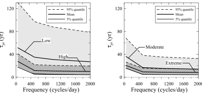
For all levels of aggressiveness and traffic frequencies, the KS-test has shown that the time to transition from pit to crack follows a lognormal distribution. Figure 7 presents the mean and 90% confidence interval
of τpt, for several traffic frequencies. Values between 8.3 − 51.4 years and 3.2 − 42.8 years are obtained for µτpt and στpt, respectively. In all cases, the mean and confidence interval of τpt reduce for higher values of
traffic frequency. This decrease is expected because the crack growth rate is function of f , and therefore, the intersection between dp/dτ and da/dτ occurs early when f is increased. It can also be observed that the
mean and the dispersion of τpt are smaller when environmental aggressiveness is increased. This reduction
is explained by fact that high levels of environmental aggressiveness are related with high values of imax.
Thus, when the imax leads to high values, the fatigue crack growth rate is increased producing an early
crack nucleation.
Since a crack is nucleated at the end of this stage, and the initial crack size is an input data to compute the
length of the following stage, Figure 8 depicts the PDFs of a0, for both various levels of aggressiveness and
several traffic frequencies. In all cases, the goodness-of-fit test shows that a0follows a lognormal distribution
with µa0varying between 1.6− 9 mm and σa0of 0.98−5.99 mm. The overall behavior indicates that both the
mean and standard deviation tend to higher values when the level of aggressiveness is increased (Figure 8a). This increase is expected because given the preponderance of pitting corrosion on fatigue for higher levels of aggressiveness, the transition occurs for higher initial crack sizes. From the relationship between the mean and standard deviation of a0and traffic frequency is possible to notice that both µa0and σa0 decrease when
f is increased (Figure 8b). This reduction is due to the fact that the augmentation of the traffic frequency turns the fatigue into the preponderating process, and subsequently, accelerates the pit-to-crack transition. 4.1.3. Crack growth
In all cases considered, the KS-test gives as a result that τcg follows a lognormal distribution with µτcg
varying between 1.6 − 48.6 years and στcg between 0.31 − 11.14 years. Figure 9 depicts the relationship
between the mean and the 90% confidence interval of τcg and the traffic frequencies. The overall behavior
indicates that the mean and dispersion of τcgdiminishes when traffic frequency is increased. This behavior
is explained by the fact that failure, i.e. eq. 21, is reached in a shorter period when the frequency tends to higher values (i.e. eq. 19). Furthermore, it can be noted that the mean and dispersion decrease when the level of aggressiveness is increased. This decrement is related to the fact that the size of the initial crack leads to larger values for higher levels of environmental aggressiveness, and therefore, the time to reach failure is lower.
For all traffic frequencies and levels of environmental aggressiveness, the KS-test shows that the size of the
critical crack at which the RC member reaches the bending limit state, ac, follows a Weibull distribution
with mean and standard deviation of 11.86 and 0.97 mm, respectively. This non dependency of f and environmental aggressiveness is expected because the bending limit state depends mainly on the effective cross section of the bar.
4.2. Total corrosion-fatigue lifetime
The goodness-of-fit test demonstrates that τT follows a lognormal distribution with mean varying between
35.8 − 448.8 years and standard deviation between 49 − 264.7 years. The PDFs of τT for various levels of
aggressiveness and f = 500 cycles/day are depicted in Figure 10a. As expected, µτT and στT decrease
when the level of aggressiveness is increased. Figure 10b presents the mean of τT for both, various levels
of aggressiveness and traffic frequencies. In general, the critical time, τT, occurs earlier when the traffic
frequency is augmented.
The relationship between the mean of τT and the level of aggressiveness is plotted in Figure 11a. It should
be noted that the mean of τTwithout considering fatigue damage (i.e. f = 0 cycles/day), is also included. The
increase of traffic frequency induces an appreciable reduction of µτT, in particular, in environments with low
aggressiveness. By taking as a reference the case without considering fatigue damage, it is possible to estimate the additional lifetime reduction induced by the coupled action of corrosion and fatigue (Figure 11b). The additional reduction of τT is high for smaller levels of aggressiveness and bigger traffic frequencies. It can be also noticed that considering the coupled effect of corrosion and fatigue can represent an additional lifetime reduction from 4 − 43%. Considering the effect of corrosion and fatigue does not produce an appreciable additional lifetime reduction for both smaller traffic frequencies and very aggressive environments. However, for traffic frequencies between 500−2000 cycles/day, the coupled effect of corrosion-fatigue induces additional
lifetime reductions between 21−43% of τT. These results strengthen the importance of including the coupled
corrosive environments under cyclic loading.
The percentage of participation of each stage in the total corrosion-fatigue life is estimated by the ratios of the mean values (Figure 12). In all cases the participation is meanly due to τcp, followed by τpt and τcg. Whereas for τcp, the participation decreases when the level of aggressiveness is increased, for τpt and τcg, it grows when the level of environmental aggressiveness is augmented. This behavior seems logical because an increment in the level of environmental aggressiveness accelerates the time to corrosion initiation and, subsequently, augments the participation of τpt and τcg. By considering the relationship between τcp and f , the percentage of participation of τcp increases when the traffic frequency grows. Contrary, for τpt and τcg, their percentages decrease when f leads to higher values. This behavior is explained by the fact that larger traffic frequencies reduce the length of the crack nucleation and propagation stages. To conclude, given the larger impact of the time to corrosion initiation and pit nucleation on the total corrosion-fatigue life (i.e. 47
to 92% of τT), the maintenance efforts must be directed towards controlling this stage of the process.
The failure probability of the girder, pf is plotted in Figure 13. It can be observed that the importance of traffic frequency on the failure probability for higher frequencies is minor. For instance, for a time window of 100 years, a moderate level of aggressiveness, without considering fatigue damage, a failure probability
of 2.7×10⁻² is obtained; for the same conditions but different frequencies, failure probability becomes
1.6×10⁻¹, 3.4×10⁻¹, 3.5×10⁻¹ and 3.7×10⁻¹ for traffic frequencies of 50, 500, 1000 and 2000 cycles/day,
respectively. That means, the failure probability is increased by 6, 12.5, 13.1 and 13.5 times for the traffic frequencies of 50, 500, 1000 and 2000 cycles/day, respectively. Whereas this difference varies considerably between 50 and 500 cycles/day, for values between 500 and 2000 cycles/day the increment is not significant. From these results it is possible to affirm that, although the coupled effect of corrosion and fatigue causes
a significant increase of pf, there is a limit after which the increase of f does not produce an appreciable
change in pf.
The influence of reinforcement, As, on failure probability for a traffic frequency of 1000 cycles/day is
plotted in Figure 14. If pf t represents the target failure probability -i.e. pf t = 10−4, and a lifetime of 50 yr is chosen, it can be observed from Figure 14 that the reinforcement resulting from the design does not
assures pf t. For the case of low aggressiveness (Figure 14a), increasing As can guarantee this condition.
Nevertheless, although increasing As tends to amplify the time to reach pf t, for the other levels the failure probability is lower than pf t. Therefore, to ensure pf tduring the lifetime of the structure, it is necessary to implement other countermeasures such as inspection and maintenance programs for corrosion control.
5. Conclusions
The combined action of corrosion and fatigue influences strongly the structural performance of RC struc-tures and reduces substantially their lifetime. In this paper, a new model that couples these two phenomena is developed and the consequences on the life-cycle of RC structures are assessed. The model takes into ac-count the interaction between the following processes: (1) corrosion induced by chloride ingress, (2) concrete cracking resulting from the accumulation of corrosion products and (3) reinforcement fatigue produced by cyclic loading. The corrosion-fatigue deterioration process is divided within the following three stages: (1) corrosion initiation and pit nucleation, (2) pit-to-crack transition and (3) crack growth. Corrosion initiation is induced by chloride ingress causing the nucleation of a pit. Pit-to-crack transition is achieved when the crack growth produced by cyclic loading becomes the preponderating process. A crack is nucleated at the end of this stage. Finally, crack growth ends when the crack size causes the structural failure.
In order to illustrate the model, a bridge girder located in several chloride-contaminated environments was studied. The time-dependant reliability analysis of the girder included the random nature of the material parameters, the loading scheme and the environmental conditions; the solution was found by using Monte-Carlo simulation. After the analysis, it was noted that the failure probability depends highly on the maximum corrosion rates, surface chloride concentration and traffic frequency.
The results also show that the time to corrosion initiation is highly influenced by the coefficient of variation of the chloride surface concentration. The mean of the time to pit nucleation had a smaller value in comparison to the mean of the time to corrosion initiation; therefore, it is possible to affirm that the length of this sub-stage can be neglected. It was also observed that pit-to-crack transition and crack growth occur early when both the level of aggressiveness and traffic frequency are increased. Regarding external loading, it was remarked that for traffic frequencies between 500 − 2000 cycles/day, the coupled effect of corrosion-fatigue becomes paramount by leading to additional lifetime reductions between 21 − 43%. However, there
is a limit after which the increase of traffic frequency does not produce an appreciable change in the failure probability.
Finally, it was observed that if the target failure probability is set as 10−4, for a structure with a lifetime of 50 years, the structural configuration selected does not reach this value for all environmental conditions considered. Therefore, to guarantee the operation above a predefined target failure probability it is necessary to implement countermeasures such as inspection and maintenance programs for corrosion control.
References
[1] Schijve J. Fatigue of structures and materials in the 20th Century and the state of the art. Int J Fatigue 2003;25:679–702. [2] Suresh S. Fatigue of Materials. 2nd ed. Cambridge: Cambridge University Press; 1998.
[3] Jones DA. Principles and prevention of corrosion. New York: Macmillan Publishing Co; 1992. [4] Clifton JR. Predicting the service life of concrete. ACI Mater J. 1993;90:611–7.
[5] Fang C, Lundgren K, Chen L, Zhu C. Corrosion influence on bond in reinforced concrete. Cem Concr Res 2004;34:2159–67. [6] Bastidas-Arteaga E, S´anchez-Silva M, Chateauneuf A, Ribas Silva M. Coupled reliability model of biodeterioration, chloride
ingress and cracking for reinforced concrete structures. Struct Saf 2007, in press.
[7] Gangloff RP. Environmental cracking corrosion fatigue. in: Baboian R, editor. Corrosion Tests and Standards: Application and Interpretation. 2nd ed. West Conshohocken: ASTM International; 2005, p. 302–21.
[8] Rajasankar J, Iyer NR. A probability-based model for growth of corrosion pits in aluminium alloys. Eng Fract Mech 2006;73:553–70.
[9] Apostolopoulos C, Dracatos P, Papadopoulos M. Low cycle fatigue behavior of corroded reinforcing bars S500s tempcore. In: Proceedings of the 6th international conference, high technologies in advanced metal science and engineering, St. Petersburg: Russia; 2004. p. 177–184.
[10] Goswami TK, Hoeppner DW. Pitting corrosion fatigue of structural materials. In: Chang CI, Sun CT, editors. Structural integrity in aging aircraft. New York: ASME; 1995, p. 129–39.
[11] Kondo Y. Prediction of fatigue crack initiation life based on pit growth. Corr 1989;45:7–11.
[12] Chen GS, Wan KC, Gao M, Wei RP, Flournoy TH. Transition from pitting to fatigue crack growth modeling of corrosion fatigue crack nucleation in a 2024-T3. aluminum alloy. Mater Sci Eng 1996;A219:126–32.
[13] Shi P, Mahadevan S. Damage tolerance approach for probabilistic pitting corrosion fatigue life prediction. Eng Fract Mech 2001;68:1493–507.
[14] Tuutti K. Corrosion of steel in concrete. Swedish Cement and Concrete Institute 1982.
[15] Harlow DG, Wei RP. A probability model for the growth of corrosion pits in aluminium alloys induced by constituent particles. Eng Fract Mech 1998;59:305–25.
[16] Vu KAT, Stewart MG. Structural reliability of concrete bridges including improved chloride-induced corrosion models. Struct Saf 2000;22:313–33.
[17] L´opez W, Gonz´alez JA, Andrade C. Influence of temperature on the service life of rebars. Cem Concr Res 1993;23:1130–40. [18] Bastidas-Arteaga E, S´anchez-Silva M, Chateauneuf A. Structural reliability of RC structures subject to biodeterioration, corrosion and concrete cracking. In: 10th International Conference on Applications of Statistics and Probability in Civil Engineering, ICAPS 10, Tokyo:Japan; 2007.
[19] Salah el Din AS, Lovegrove JM. Fatigue of cold worked ribbed reinforcing bar – A fracture mechanics approach. Int J Fatigue 1982;4:15–26.
[20] Murakami Y, Nisitani H. Stress intensity factor for circumferentially cracked round bar in tension. Trans Jpn Soc Mech Engng. 1975;41:360–9.
[21] Zhang R, Mahadevan S. Reliability-based reassessment of corrosion fatigue life. Struct saf 2001;23 77–91.
[22] European standard. Eurocode 1 and 2: Basis of design and actions on structures and design of concrete structures. AFNOR. april 2004.
[23] McGee R. Modelling of durability performance of Tasmanian bridges. In: Melchers RE, Stewart MG, editors. Applications of statistics and probability in civil engineering. Rotterdam: Balkema; 2000. p. 297–306.
[24] Geocisa and Torroja Institute, Contecvet: A validated users manual for assessing the residual service life of concrete structures. Manual for assessing corrosion-affected concrete structures. Annex C Calculation of a representative corrosion rate. EC Innovation Program IN309021. British Cement Association, UK, 2002.
[25] Kent DC, Park R. Flexural members with confined concrete. J Struct Div ASCE 1971; 97:1969–90. [26] Melchers RE. Structural reliability-analysis and prediction. Chichester: Ellis Horwood; 1999.
[27] Hong HP. Assessment of reliability of aging reinforced concrete structures. J Struct Eng ASCE 2000; 126:1458–65. [28] Thoft-Christensen P. Stochastic Modelling of the Crack Initiation Time for Reinforced Concrete Structures. In: ASCE
2000 Structures Congress, Philadelphia, USA 2000. p. 1–8.
[29] Stewart MG. Spatial variability of pitting corrosion and its influence on structural fragility and reliability of RC beams in flexure. Struct Saf 2004;26:453–470.
List of Tables
– Table 1. Design load and material constants.– Table 2. Description of the studied environments.
– Table 3. Probabilistic models of the variables used in the model.
List of Figures
– Fig. 1. Scheme of corrosion-fatigue deterioration process in RC structures. – Fig. 2. (a) Rate competition criterion. (b) Time-variant corrosion rate. – Fig. 3. Flowchart of the proposed model.
– Fig. 4. Configuration of the bridge girder.
– Fig. 5. PDFs of τini for various levels of aggressiveness.
– Fig. 6. Relationship between µτini and µCs in terms of: (a) COV(Dcl), and (b) COV(Cs).
– Fig. 7. Mean and 90% confidence interval of τpt for several traffic frequencies.
– Fig. 8. PDFs of a0 for: (a) various levels of aggressiveness and f = 50 cycles/day; (b) low level of
aggressiveness and various traffic frequencies.
– Fig. 9. Mean and 90% confidence interval of τcg for several traffic frequencies.
– Fig. 10. (a) PDFs of τT for various levels of aggressiveness and f = 500 cycles/day; (b) mean of τT for
both, various levels of aggressiveness and traffic frequencies.
– Fig. 11. (a) Mean of τT for various traffic frequencies. (b) Additional lifetime reduction induced by the
coupled action of corrosion and fatigue.
– Fig. 12. Percentage of participation of each phase in the total corrosion-fatigue life. (a) Low aggressiveness. (b) Extreme aggressiveness.
– Fig. 13. Time-dependent structural reliability of the considered bridge girder.
– Fig. 14. Influence of positive steel reinforcement area on failure probability for several levels of aggres-siveness: (a) low, (b) moderate.
Table 1
Design load and material constants.
Variable Value Description
Pk 150 kN Characteristic punctual design load
Est 200000 N/mm2 Elastic modulus of steel
f0
ck 30 MPa Characteristic concrete compression strength
fyk 500 MPa Characteristic steel strength
γc 22 kN/m3 Specific weight of concrete
γp 18 kN/m3 Specific weight of pavement
νc 0.2 Concrete Poisson ratio
ρst 8000 kg/m3 Density of steel
Table 2
Description of the studied environments.
Level of Description Cs [23] imax [24] c[22]
aggressiveness kg/m3
µA/cm2
mm Low structures located at 2.84 km or more from the coast; sea spray
carried by the wind is the main source of chlorides.
0.35 0.5 40
Moderate structures located between 0.1 and 2.84 km from the coast whithout direct contact with seawater.
1.15 2 45
High structures situated to 0.1 km or less from the coast, but with-out direct contact to seawater. RC structures subject to de-icing salts can also be classified in this level.
2.95 5 50
Extreme structures subject to wetting and drying cycles; the processes of surface chloride accumulation are wetting with seawater, evaporation and salt crystallization.
7.35 10 55
Table 3
Probabilistic models of the variables used in the model.
Variable Distribution Mean COV Source
P Lognormal 115 kN 0.20 f0 c Normal 40 MPa 0.15 [26] fy Normal 600 MPa 0.10 [26] Cth Uniform 0.90 kg/m3 0.19 [16] Cs Low Lognormal 0.35 kg/m3 0.50 [23] Moderate Lognormal 1.15 kg/m3 0.50 [23] High Lognormal 2.95 kg/m3 0.50 [23] Extreme Lognormal 7.35 kg/m3 0.70 [23] Dcl Lognormal 63 mm2/yr 0.75 [27] ρrust Normal 3600 kg/m3 0.10 [28] tpor Lognormal 12.5×10⁻⁶m 0.20 [28] α Gumbel 5.65 0.22 [29]
CYCLIC LOAD CHLORIDE INGRESS RC CRACKING Chloride ingress: pH reduction, steel depassivation Cyclic load: crack nucleation and propagation Pit-to-crack transition FAILURE Corrosion initiation Pit nucleation and growth Crack nucleation and crack growth Excessive cracking of concrete: acceleration of icorr Concrete crack initiation Corrosion rate: generation of corrosion products 1. Corrosion initiation and pit nucleation,
v
cp2. Pit-to-crack transition,
v
pt 3. Crack growth,v
cgTotal corrosion-fatigue life,
v
TFig. 1. Scheme of corrosion-fatigue deterioration process in RC structures.
vpn
d
a
/d
v
and
d
p
/d
v
Time
da/dv dp/dv vpt vcpCorros
ion
ra
te
Time
Vu and Stewart, (2000), iini(v)
Bastidas-Arteaga et al, (2007), icorr(v)
imax
d0 d0
p*v +
Uncorroded
bar Pit shape
vsc
vini
vini
a
b
Increasing of the chloride concentration at the cover depth until corrosion initiation
Reduction of steel area induced by corrosion
Accumulation of corrosion products leading to cracking Nucleation and growth
of the pit
Increasing of corrosion rate as a result of
several concrete cracking
Evaluation of the rate competition criterion
Transition between pit and crack. Nucleation and growth of the
crack until a critical value
FAILURE
Structural configuration Loading scheme
(e.g. cyclic load)
Environmental features (e.g. surface chloride
concentration)
INPUT DATA
Fig. 3. Flowchart of the proposed model.
d d’ b = 400 mm h = 1000 m m hs= 200 mm hp= 160 mm lb= 2000 mm Slab Pavement c b’’ h’’ 8 d0=25 mm 4 d0=20 mm d0= 10 mm Stirrups:
0 200 400 600 800 1000
Time (yr)
0 0.002 0.004 0.006f
vin i(
v
)
0 20 40 60 80Time (yr)
0 0.02 0.04 0.06f
vin i(
v
)
Moderate
o"="42705"yr u = 279.2 yrLow
o"="5:508"yr u = 368.3 yrExtreme
o"="4803"yr u = 51.4 yrHigh
o"="8308"yr u = 123.2 yrFig. 5. PDFs of τinifor various levels of aggressiveness.
a
b
0 2 4 6 8Mean of C
s(kg/m
3)
0 200 400 600M
ea
n
o
f
v
in i(
y
r)
COV = 0.30 COV = 0.50 COV = 0.75 0 2 4 6 8Mean of C
s(kg/m
3)
0 200 400 600M
ea
n
of
v
in i(
y
r)
COV = 0.30 COV = 0.50 COV = 0.700 400 800 1200 1600 2000
Frequency (cycles/day)
0 40 80 120v
pt(
yr
)
95% quantile Mean 5% quantile Low High 0 400 800 1200 1600 2000Frequency (cycles/day)
0 40 80 120v
pt(
y
r)
95% quantile Mean 5% quantile Moderate ExtremeFig. 7. Mean and 90% confidence interval of τptfor several traffic frequencies.
0 4 8 12 16
a (mm)
0 0.2 0.4 0.6f
a0(v
)
Low Moderate High Extremea
b
0 2 4 6a (mm)
0 0.2 0.4 0.6f
a0(v
)
f =50/day f =500/day f =1000/day f =2000/day o"="4075"mm u = 1.55 mm o"=";028"mm u = 5.99 mm o"="9056"mm u = 4.58 mm o"="4075"mm u = 1.55 mm o"="30:;"mm u = 1.16 mm o"="3082"mm u = 0.98 mm o"="3096"mm u = 1.07 mm o"="6092"mm u = 2.92 mmFig. 8. PDFs of a0for: (a) various levels of aggressiveness and f = 50 cycles/day; (b) low level of aggressiveness and various
0 400 800 1200 1600 2000
Frequency (cycles/day)
0 20 40 60v
cg(
y
r)
95% quantile Mean 5% quantile Low High 0 400 800 1200 1600 2000Frequency (cycles/day)
0 20 40 60v
cg(
y
r)
95% quantile Mean 5% quantile Moderate ExtremeFig. 9. Mean and 90% confidence interval of τcg for several traffic frequencies.
500 400 300 200 100 0 2000 0 1000 500 Low Moderate High Extreme
M
ea
n
of
v
T(yr)
Tr
af
fic
fr
eq
ue
nc
y
(c
yc
le
s/d
ay
)
Level
of
aggre
ssiven
ess
0 100 200 300 400 500Time (yr)
0 0.01 0.02 0.03f
vT(v
)
Low Moderate High Extreme o"="39.7 yr u = 49.3 yr o"="397.0 yr u = 268.7 yr o"="213.5 yr u = 206.4 yr o"="76.3 yr u = 100.8 yra
b
Fig. 10. (a) PDFs of τT for various levels of aggressiveness and f = 500 cycles/day; (b) mean of τT for both, various levels of
0 400 800 1200 1600 2000
Frequency (cycles/day)
0 10 20 30 40 50A
d
d
it
io
n
al
r
ed
u
ct
io
n
o
f
v
T(%)
Low Moderate High Extremea
b
Level of aggressiveness
0 200 400 600o
vT(y
r)
f =0/day f =50/day f =500/day f =1000/day f =2000/dayLow Moderate High Extreme
Fig. 11. (a) Mean of τT for various traffic frequencies. (b) Additional lifetime reduction induced by the coupled action of
corrosion and fatigue.
a
b
Frequency (cycles/day)
0 20 40 60 80 100P
er
ce
n
ta
g
e
o
f
p
ar
ti
ci
p
at
io
n
vcp vpt vcg 50 500 1000 2000Frequency (cycles/day)
0 20 40 60 80 100P
er
ce
nt
age
of
pa
rt
ic
ip
at
io
n
vcp vpt vcg 50 500 1000 2000Fig. 12. Percentage of participation of each phase in the total corrosion-fatigue life. (a) Low aggressiveness. (b) Extreme aggressiveness.
0 40 80 120
Time (yr)
0 0.2 0.4 0.6 0.8 1F
ai
lu
re
p
ro
b
ab
il
it
y
f = 0 /day f = 50 /day f = 500 /day f = 1000 /day f = 2000 /dayHigh
Extreme
0 100 200 300 400Time (yr)
0 0.2 0.4 0.6 0.8 1F
ai
lure
pr
oba
b
il
it
y
f = 0 /day f = 50 /day f = 500 /day f = 1000 /day f = 2000 /dayLow
Moderate
Fig. 13. Time-dependent structural reliability of the considered bridge girder.
0 20 40 60 80 100
Time (yr)
1x10⁻⁵ 1x10⁻⁴ 1x10⁻³ 1x10⁻² 1x10⁻¹F
ai
lu
re
p
ro
b
ab
il
it
y
(
p
f)
8 bars10 bars 12 bars 14 barsa
p
f t 0 10 20 30 40Time (yr)
1x10⁻⁵ 1x10⁻⁴ 1x10⁻³ 1x10⁻² 1x10⁻¹F
ai
lu
re
p
ro
b
ab
il
it
y
(
p
f)
8 bars10 bars 12 bars 14 barsp
f tb
Fig. 14. Influence of positive steel reinforcement area on failure probability for several levels of aggressiveness: (a) low, (b) moderate.