∆
-TSR: a description of spatial relationships between objects
for image retrieval
∗
Nguyen Vu Hoang
1,2, Val´erie Gouet-Brunet
2, Marta Rukoz
1,3, Maude Manouvrier
11: LAMSADE - Universit´e Paris-Dauphine - Place de Lattre de Tassigny - F75775 Paris Cedex 16 2: CEDRIC/CNAM - 292, rue Saint-Martin - F75141 Paris Cedex 03
3: Universit´e Paris Ouest Nanterre La D´efense - 200, avenue de la R´epublique - F92001 Nanterre Cedex
[email protected] , [email protected] , [email protected], [email protected]
August 10, 2009
Abstract
This article presents ∆-TSR, a new image content representation exploiting the spatial relationships existing between its objects of interest. This approach provides two types of descriptions: with ∆-TSR3D,
images are represented by geometric relationships between triplets of objects using triangle angles, while ∆-TSR5D enriches ∆-TSR3D by exploiting the orientation of the objects. The approach is generalized to
polygonal spatial relationships, from triplets to tuples of objects. All these descriptions are invariant to translation, 2D rotation, scale and flip. A semi-local representation of the relationships is also proposed, making the description robust to viewpoint changes, if required by the application. ∆-TSR can be applied not only to symbolic images (where objects are represented by labels or icons) but also to contents represented by low-level visual features such as interest points. In this work, we evaluate ∆-TSR for image and sub-image retrieval under the query-by-example paradigm, on contents represented with interest points in a bag-of-features representation. We show that ∆-TSR improves two state-of-the-art approaches, in terms of quality of retrieval as well as of execution time. The experiments also highlight its effectiveness and scalability against large image databases.
Keywords: CBIR, spatial relationships, local image descriptors, fast retrieval
1
Introduction
Under the query-by-example paradigm, Content-Based Image Retrieval (CBIR) aims at retrieving a ranked list of similar images from an example and a set of images. One variant concerns the retrieval of sub-images or objects of interest identical or similar to a query sub-image or object. This scenario is a challenging problem due to the difficulty of representing, matching and localizing objects in potentially large-scale collections and on under viewpoint changes, partial occlusion and cluttered background. Literature on image content representation is very large, see for example [4] for a survey. In this work, we investigate approaches that focus on the representation of the spatial layout in image contents. The spatial relationships between image objects are a key point of image understanding. They offer a strong semantic which comes to enrich the low-level techniques of image visual content representation. To address this topic, many solutions have been proposed for describing
∗This work is done within the French Federation WISDOM (2007-2010) and is supported by the French project ANR MDCO DISCO (2008-2010).
the spatial relationships between the objects, which can be symbolic (e.g. a tree or a person) as well as low-level features (e.g. salient points); we revisit them in section 1.1. In this work, we present ∆-TSR, which is a description of the triangular spatial relationships between objects. The main characteristics of this approach and the paper outline are summarized in section 1.2.
1.1
State of the Art
First, we summarize several propositions for describing the spatial relationships between symbolic objects in section 1.1.1. Second, because we evaluate our approach for sub-image retrieval in images where the contents are represented with sets of salient points, we give a panorama of the existing techniques representing spatial relationships between these particular objects in section 1.1.2.
1.1.1 Spatial relationships between objects in images
Among the more known categories, we can mention the directional [2, 8], topological [5], geometrical [7] and orthogonal [3] relationships. In particular, the geometrical ones lend themselves well to invariance to certain geometrical image transformations, in particular to rotation. In these approaches, the objects are represented by their centroid and metric measures between these points are exploited to characterize the relationships between couples or triplets of objects. Our work is inspired by the geometrical approach TSR (Triangular
Spatial Relationship) which characterizes the spatial relationships between object triplets by angles built from
the triangle formed by the object centroids [7, 16]. Let Oibe an object represented by the spatial coordinates of
its centroid and by a code Liof its label; two objects with different coordinates may have the same label. In the
following, for the sake of simplicity, we use indistinctly Oifor the object and for its centroid. In TSR approach,
the triangle formed by three objects O1, O2 and O3 is represented by one of the six possible quadruplets (L1,
L2, L3, θ) where, L1, L2 and L3 are the label codes of O1, O2 and O3 respectively, and θ is the smallest angle
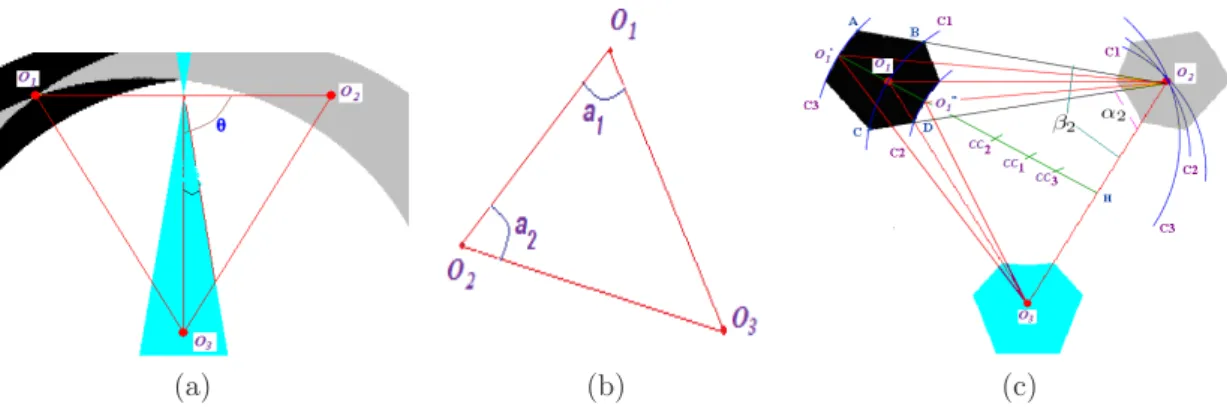
subtended at the midpoint resulting from O3 to the side O1O2 of the triangle – see Fig. 1(a). The objects are
then ordered by their labels in order to always consider the same arrangement of object triplet. An image is thus encoded by the set of quadruplets representing the triangular spatial relationships between all the possible triplets of objects. This representation is invariant to rotation, translation, scaling and flipping. To minimize the storage space and speed up the search time, the continuous domain [0◦, 90◦] associated with θ is split into
Dθ classes and each quadruplet is represented by a unique and distinct single key defined by Equation 1:
K = Dθ(L1− 1)(NL)2+ Dθ(L2− 1)NL+ Dθ(L3− 1) + (Cθ− 1) (1)
Where Cθ ∈ [1, Dθ] is the class number to which a specific value of θ belongs, NL the number of object
labels in the database and (L1, L2, L3) ∈ [1, NL]3⊂ N3 with L1≥ L2≥ L3.
The discretization of the continuous domain of θ allows to take into account the possible variations of θ and to consider mismatch between the quadruplets representing the same objects with the same spatial relationships during matching/retrieval process. The set of keys makes thus possible to seek images and sub-images similar to a query image. Nevertheless, the number of stored keys per image is (NO× (NO− 1) × (NO− 2)/6) = O(NO3),
with NO the number of objects in the database. Keys are therefore stored in a B-tree. Via this structure, the
authors indicate that search time is in O(NQlogbNK), where NQis the number of TSR quadruplets in the query
image Q, NK is the total number of keys in the B-tree of order b.
This approach has two drawbacks. By one hand, the tolerance interval of θ is included into the key formula of Equation 1. As a result, if the user wants to change the interval values, all keys have to be recalculated and restored. By the other hand, because of θ ’s definition, even a little variation of θ can produce a large variation zone of triangles defined as similar, as shown in Fig. 1(a). This figure represents the variation zone of an equilateral triangular O1O2O3 with a tolerance interval of θ equal to 10◦. The black zone represents the
possible variations of O1, the grey zone the possible variations of O2and the blue one, the variation zone of O3:
if O2and O3 are fixed, all triangles formed by O2, O3and all the points O1 of the black zone are considered as
similar triangles in the TSR approach.
1.1.2 Image description with Bags of Features
There exist many solutions for image description based on sets of sparse local features, see for example the recent survey on local invariant feature detectors [20]. More recently, other approaches have exploited a bag-of-features representation of the local descriptors (BoF), introduced by [19]. This concept comes from text retrieval and consists in building a visual vocabulary (a codebook) from quantized local descriptors and in representing the image by a vector of fixed size involving the frequency of each visual word of this vocabulary. The concept is usually applied to object recognition, after having trained descriptors to be tolerant to inter and intra-class variability when dealing with recognition of classes of objects. This representation has the advantage of locally describing the image content while only involving one feature vector per image. Moreover, it generates a very sparse feature space that can be accessed quickly with inverted files.
The main drawbacks of the BoF representation are that it disregards all information about the spatial layout of the local features and that the discriminative power of local descriptors is limited due both to quantization and to the large number of images. Usually, spatial information is reintroduced a posteriori at the last stage of retrieval on remaining matching features, by performing geometric verification or registration, as in [12] with the Hough transform or in [15] with an improved version of RANSAC. This step is particularly computational expensive, given that it is applied on a lot of features which do not verify required spatial relationships. To address this problem, the authors of [22] proposed a novel scheme to bundle the well-known SIFT features into local groups by using MSER (Maximally Stable External Region) detection. These bundled features are repeatable and much more discriminative than an individual SIFT feature. In matching bundled features, the authors define the matching score for measuring similarity of two bundled features. This score consists of membership term and a geometric term and it can be parameterized by a weighting parameter.
Incorporating spatial information a priori into the content description is another very relevant solution. Enriching the description with such information has the advantage of better filtering the local features to retrieve but it may remain quite challenging because of the potential expensive combinatorial description involved. Several kinds of solutions have been proposed for this category of solutions. In [18], the authors increase the visual words vocabulary with “doublets”, i.e. pairs of visual words which co-occur within a local spatial neighborhood. Similar ideas were proposed in [17] with correlograms describing pairwise features in increasing neighborhoods. In [24], an invariant descriptor is proposed to model the spatial relationship of keypoints (visual words), by computing the average of the spatial distribution of a cluster center (called keyton) relative to all the keypoints of another cluster center. The relative spatial distribution is computed by separating the image’s plane in co-centered circles using a keypoint as origin, each co- centered circle representing a relative distance and being broken into four equal parts. In [9] the authors propose a higher-level lexicon, i.e. visual phrase lexicon, where a visual phrase is a meaningful spatially co-occur pattern of visual words. This higher-level lexicon is less ambiguous than the lower-level one. Due to the spatial dependency of the visual data, a likelihood ratio test method is proposed to evaluate the significance of a visual word set. In addition, to overcome the complexity in searching for the meaningful patterns (the total number of possible word-sets is exponential to the cardinality of visual words lexicon), they develop an improved frequent item set mining (FIM) algorithm based on the new criteria to discover significant visual phrases in a very efficient way. In [11] the authors propose to extract progressively higher-order features, representing spatial relationships between pixels or patches, during the first-order feature (bag-of local feature descriptors) selection for object categorization. Their idea is to avoid exhaustive extraction of higher-order features and then exhaustive computation. The second-order features used are non-parametric spatial histograms describing how co-occurrences of first-order features vary in distance or with distance approximately in log scale with four directional bins (above, below, to the left and to the right).
Other approaches describe the spatial layout into a hierarchy of features. In [1], the geometry and visual appearance of objects is described as a hierarchy of parts (the lowest level being represented with local features), with probabilistic spatial relations linking parts to subparts. Similarly in [10], the pyramid match kernel of Grauman and Darrel [6] is adapted to create a spatial pyramidal image where images are recursively decomposed into sub-regions represented by BoF. The authors of [14] propose a hierarchical model that can be characterized as a constellation of BoF and that is able to combine both spatial and spatio-temporal features of videos. In [26], the authors address the tasks of detecting, segmenting and parsing deformable objects in images. A probabilistic object model is proposed, called the Hierarchical Deformable Template (HDT), which represents the object appearance at different scales over a hierarchy of structures, from elementary to more complex structures: low-level patches (gray values, gradients and Gabor filters), short-range shapes (triplets of points described by their relative angles and scales), mid-level regions (mean and variance of regions and patches) and long-range shapes characterized with triangular relationships. This set of structures were initially proposed in [25] but in [26], the learning model proposed is more sophisticated: a probability distribution is defined over the hierarchy to quantify the variability in shape and appearance of the object at multiple scales. Experimental evaluations of this model were performed mainly for detection and segmentation on public image databases (Weizmann Horse dataset and Cows). The model was also compared to state-of-the-art techniques for these tasks: among approaches that do not employ a priori information, the proposed approach provides the best results (94.7 % of segmentation accuracy).
While all the previous approaches were designed for learning of object classes for image categorization, [21] introduces, for CBIR, some spatial information into the visual description by first applying a spatial clustering on salient points in the image, providing a set of “visual constellations” that gather the points of the same neighborhood and secondly by characterizing each constellation with a classical bag-of-features representation. Note that this last approach was evaluated in terms of quality of the images retrieved, but time retrieval was not considered.
Among the different approaches presented above, the approach proposed in [26] is the only one that also exploits triplets of points as visual structures, similarly to our solution ∆-TSR. But the objectives of the authors are clearly different: in our approach, we are able to perform image or sub-image retrieval in collections of images, with a dynamic selection of the part to retrieve and without any a priori knowledge on the object or image part to be searched. Additionally, the coding of these triplets is different, with the aim of fast online retrieval of image parts in large collections, under the query-by-example paradigm.
1.2
Contributions and outline of the paper
The objective of this work is to propose an efficient and effective representation of the spatial layout of objects for image or sub-image retrieval in large collections of images, under the query-by-example paradigm. The proposed approach is called ∆-TSR and is implemented in this paper on objects which are local visual features based on salient points represented in a BoF model; it is presented in section 2. ∆-TSR uses the same idea of TSR, i.e. representing image layout by the triangular relationships between its objects. However, the adopted coding has a filtering capacity higher than TSR, leading to superior performances in terms of quality of retrieval as well as of online retrieval time. On several image data sets varying from 600 to 6000 images, we demonstrate its relevance both in terms of quality of the description (Section 3) and of retrieval time (Section 4), facing TSR and a classical bag-of-features representation of visual content. Finally, Section 5 concludes.
2
Approach ∆-TSR
In section 2.1, we present the main principles of the proposed approach for describing spatial relationships between triplets of objects in images. This approach can be enriched according to several solutions described
(a) (b) (c)
Figure 1: (a) Variation zone in T SR (b) Triangular relationship of 3 objects O1, O2, O3in ∆-TSR (c) Variation
zone in ∆-TSR and its geometrical demonstration.
in section 2.2. We also generalize it to any tuples of objects in section 2.3 and then present the associated similarity measure in section 2.4. Finally, we explain our proposal for efficiently indexing this description with an access method in section 2.5.
2.1
Spatial relationship description
Taking up the idea of representing the spatial relationships between triangles of objects from the TSR approach [16], we propose a new image description called ∆-TSR3D. This approach is applicable to objects which can be
either symbolic objects represented by a point (e.g. their centroid) or low-level visual features such as interest points. Each image I of the database is represented by a set ∆-TSR3D(I) containing the signatures of all the
triangular relationships between its objects (ordered by their labels) such as:
∆-TSR3D(I) = {Sa(Oi, Oj, Ok)/Oi, Oj, Ok∈ I; i, j, k ∈ [1, NI]; Li≥ Lj≥ Lk} (2)
with NI the number of object in image I. The other variables are the same as those defined at Equation 1.
The triangular relationship between three objects Oi, Ojand Ok, is represented by a 3-dimensional signature:
Sa(Oi, Oj, Ok) = (K1, K2, K3) ; ∀i, j, k ∈ [1, NI] (3) with K1= (Li− 1)(NL)2+ (Lj− 1)NL+ (Lk− 1) K2= ai; K2∈ [0◦, 180◦] K3= aj; K3∈ [0◦, 180◦]
ai, aj are the angles of vertices Oi, Oj respectively – see Figure 1(b). They must satisfy the following
conditions1: (ai, aj∈ N) ∧ (ai, aj∈ [0◦, 180◦]) Li= Lj=⇒ ai≥ aj Lj= Lk=⇒ ai≥ 180◦− ai− aj
K1 coding can encompass a large number of triangles: with NL = 1000 (number of labels used in most of
the experiments of sections 3 and 4), K1 can represent 1 billion of triangles, easily manageable with integer
type. While the same key K can be associated with different triangles by setting a tolerance interval in TSR [16], in our approach each signature is associated with a single triangle and its symmetric. Moreover, instead of computing a key which depends on the tolerance interval (coded by Dθand Cθin the key formula of TSR – see
Eq. 1), our 3-dimensional signature Sa is independent from the tolerance interval, called δ
a. Thus, changing 1Note that, in order to take less memory and to accelerate the process, we choose ai and aj in N instead of R. Moreover, our experiments using real type provided no improvement.
δa has no impact on the image description and indexing. In return, δa is used to define the similarity between
triangles. We consider as similar triangles of triangle TQ all the triangles TI whose angles verify the tolerance
constraints defined by:
α1 = max(ai(TQ) − δa, 0◦) ≤ ai(TI) ≤ β1= min(ai(TQ) + δa, 180◦)
α2 = max(aj(TQ) − δa, 0◦) ≤ aj(TI) ≤ β2= min(aj(TQ) + δa, 180◦)
ak(T ) = 180◦− aj(T ) − ai(T ); ∀T = TQ, T I
α3 = max(ak(TQ) − δa, 0◦) ≤ ak(TI) ≤ β3= min(ak(TQ) + δa, 180◦)
(4)
These constraints can be demonstrated geometrically; we demonstrate the validity of the variation zone for
O1. Let us consider an equilateral triangle O1O2O3 represented in Fig. 1(c). The black zone represents the
possible variation zone of O1when O2and O3are fixed, and with δa = 10◦. H represents the midpoint of O2O3,
O10 corresponds to the point such as O2\O10O3 = α1 and O100 to the point such as O2\O100O3 = β1. Let C1,
C2, C3 be the arcs of circles circumscribing triangles O1O2O3, O10O2O3 and O1”O2O3. Every point P on arcs
C1 is such that \O2M O3 = \O2O1O3. Therefore, all arcs of circles with a center CC on the median O1H and
which pass through the area bounded by arcs of circles C2 and C3 contain M such that α1≤ \O2M O3β1. This
represents the set E1of points O1 that validates the first constraint of tolerance above – see the first line in Eq.
(4). All triangles similar to O1O2O3 must also satisfy the second constraint of tolerance. Let O2B and O2D
be the lines such that \BO2O3= β2 etDO2\O3= α2. Then, all points O1 in the area bounded by these 2 lines
verify α2 ≤ \O1O2O3 ≤ β2. This corresponds to the set E2 of points validating the second constraint. In the
same way, we can find set E3of points validating the third condition of tolerance. As a result, the intersection
of E1, E2 and E3represents a (black) region containing all points O1which allow to construct a triangle similar
to the initial triangle O1O2O3. As O1O2O3 is equilateral, areas of variation of the 3 vertices are identical. For
another type of triangle, we can also define its areas of geometrical variations.
Note that if angles are not considered in the signature, we obtain a signature ∆-TSR1D, similar to those
proposed in [17, 18] (see section 1.1.2), but which considers co-occurrences of triplets instead of doublets of objects, such as:
∆-TSR1D(I) = {S`(Oi, Oj, Ok)/Oi, Oj, Ok∈ I; i, j, k ∈ [1, NI]; Li≥ Lj ≥ Lk} (5)
with: S`(O
i, Oj, Ok) = (K1) ; ∀i, j, k ∈ [1, NI] (6)
2.2
Improvements of the description
∆-TSR3D can be improved or adapted according to the application. We present two possible improvements in
sections 2.2.1 and 2.2.2.
2.2.1 Description ∆-TSR5D
In ∆-TSR3D, the objects of interest are exclusively represented by their centroids. For a large palette of objects,
it is possible to consider an orientation: if the object is symbolic, we can consider the orientation of its largest segment or the average orientation computed on points inside the object; with salient points, a main orientation can be computed from the local gradient around the point, as in the SIFT description for example [12].
By representing an object by its centroid plus its orientation, we propose the representation ∆-TSR5D,
which is also invariant to translation, 2D rotation, scale and flip. The triangular relationship of 3 objects
Oi, Oj, Ok whose digital labels are Li, Lj, Lkcan be represented by a 5-tuple (K1, K2, K3, K4, K5), where triplet
(K1, K2, K3) corresponds to Sa(Oi, Oj, Ok) of Equation 3. Let γlbe the orientation’s angle associated with Ol
(with respect to x axis for simplicity). K4 and K5 represent the relative orientation of Oi and Oj with respect
to Ok, in order to maintain invariance to 2D rotation. The associated description, So, is described by:
So(O
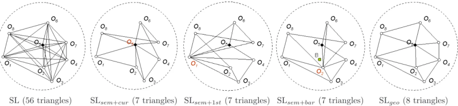
SL (56 triangles) SLsem+cur (7 triangles) SLsem+1st (7 triangles) SLsem+bar (7 triangles) SLgeo (8 triangles)
Figure 2: Illustration of the pruning strategies on a semi-local neighborhood centered on object O5 and
con-taining 8 objects. The value in parentheses is the number of triangles involved. For SLsem, the red point is the
pivot (O5for SLsem+cur, O1for SLsem+1st and O2for SLsem+bar). In the SLsem+bar triangulation, the squared
green point “B” is the barycenter of the 8 centroids.
with K1= (Li− 1)(NL)2+ (Lj− 1)NL+ (Lk− 1) K2= ai; K2∈ [0◦, 180◦] K3= aj; K3∈ [0◦, 180◦] K4= |γi− γk|; γi, γj, γk∈ [−180◦, 180◦] K5= |γj− γk|; K4, K5∈ [0◦, 360◦]
After δa, a second threshold δo is introduced for considering similarity search with K4 and K5, K4(TI)
varying in [K4(TQ) − δo, K4(TQ) + δo] and K5(TI) in [K5(TQ) − δo, K5(TQ) + δo].
Finally, the image’s global signature, noted ∆-TSR5D(I), is obtained similarly to ∆-TSR3D(I):
∆-TSR5D(I) = {So(Oi, Oj, Ok)/Oi, Oj, Ok ∈ I; i, j, k ∈ [1, NI]; Li ≥ Lj≥ Lk}
2.2.2 Selection of relevant triplets of objects
∆-TSR1D, ∆-TSR3D and ∆-TSR5D may involve triplets of objects located far away from each other in the
image. Such a representation is adequate for global image content description and retrieval, but is not for sub-image or object of interest retrieval. Here, a semi-local description of the spatial layout, that privileges smaller triangles of objects, is largely sufficient for sub-image querying and ensures more robustness to changes of viewpoint for retrieval of objects of interest represented with several triangles; objects described with BoF typically enter in this category. Let r be a radius of neighborhood; for sake of simplicity, r is a predefined parameter fixed for all objects, but it can be adapted given an idea of object’s scale, such as with the SIFT points which are extracted at specific scales. The following strategy of triangle selection is applied for each object Oi of image I:
Strategy SL: Semi-local pruning of triplets
1. Find all objects Oj in the neighborhood of Oi, i.e. dL2(Oi, Oj) ≤ r where dL2 stands for the Euclidean distance;
2. Build all the triangular relationships from the list of items {Oj} found.
One interesting consequence of this strategy is that the number of triangles of the image signature (C3
NI
by default, where NI is the number of objects in I) is considerably reduced to an average amount of NI × Cn¯3
relationships are build in a semi-local neighborhood. In each neighborhood, we can reduce the complexity of the description even more by adding other strategies of pruning, such as the two following ones:
Strategy SLsem: Pruning based on semantics
This strategy is also semi-local and keeps a triangulation that is deduced from the object’s labels, as follows: 1. Find all objects Oj in the neighborhood of Oi, as in strategy SL;
2. Sort list {Oj} by increasing order of their labels Li ;
3. Select in list {Oj} a particular object Op(pivot), according to a criteria of selection defined below. Remove
Opfrom {Oj};
4. From this list of size |{Oj}|, build all the triangular relationships (Op,Ojl,Ojm) where l = 1, .., |{Oj}|,
m = 1 if l = |{Oj}| and m = l + 1 otherwise.
We propose three alternatives for selecting pivot Op: • Strategy SLsem+cur: Consider Oi as Op;
• Strategy SLsem+1st: Take Op as the first object of list {Oj} (remember that the list is sorted on the
labels);
• Strategy SLsem+bar: Take Op as the object closest to the spatial barycenter of items in {Oj}. This
strategy is not purely based on semantics since it exploits the geometry of the objects by the way of their barycenter.
Whatever the criteria of selection of Op, strategy SLsem ensures that the size of the image signature is
reduced to an average of NI× (¯n − 1) triplets. Inside each neighborhood, we obtain a minimal set of triangles,
potentially overlapping, that connects every object Oj to three other objects at least.
Strategy SLgeo: Pruning based on geometry
Differently to strategy SLsem, this strategy provides a triangulation of the objects in the semi-local
neigh-borhood, that is directly deduced from their geometry, as follows: 1. Find all objects Oj in the neighborhood of Oi, as in strategy SL;
2. From all the possible triangles built on set {Oj}, select the subset that form a Delaunay triangulation.
A Delaunay triangulation is chosen for this strategy, because it maximizes the minimum angle of the involved triangles, thus reducing their stretching and then increasing their robustness to viewpoint changes by preserving locality. Such a triangulation ensures that the size of the image signature is reduced to an average of NI×[2(¯n−
1) − ¯e] triplets, where ¯e is the average number of objects on the convex envelope. Inside each neighborhood, we
obtain a minimal set of disjoint triangles, that form a partition of the convex envelope associated with objects
{Oj}.
Strategies SL, SLsem and SLgeo are illustrated in Figure 2 on a set of 8 objects. They are evaluated and
2.3
Generalization of ∆-TSR: ∆-PSR
“PSR” is the abbreviation for “Polygonal Spatial Relationships”, which generalizes ∆-TSR to polygonal supports of description of the spatial layout. If image I contains NI objects, we consider d objects O1, ..., Od of I
(3 ≤ d ≤ NI), which are organized to verify L1≥ ... ≥ Ld−1≥ Ld. Then, the relationship between these objects
is represented by a closed polygon composed of vertices (O1, ..., Od) where consecutive vertices are connected.
Let ai be the angle associated with each of these vertices, and γithe orientation of Oi. Note that if Li= Lj for
two objects Oiand Oj, they are sorted according to these angles and orientations. According to the information
considered, the corresponding signatures of polygons are defined as follows: S`(O 1, ..., Od) = (K1) Sa(O 1, ..., Od) = (K1, K2, ..., Kd) So(O 1, ..., Od) = (K1, K2, ..., Kd, Kd+1, ..., K2d−1) (8) with K1= Pd
i=1(Li− 1) × (NL)d−i K2= a1; K2 ∈ [0◦, 180◦] K3= a2; K3 ∈ [0◦, 180◦] ... Kd= ad−1; Kd∈ [0◦, 180◦] Kd+1= |γ1− γd|; Kd+1∈ [0◦, 360◦] Kd+2= |γ2− γd|; Kd+2∈ [0◦, 360◦] ... K2d−1= |γd−1− γd|; K2d−1∈ [0◦, 360◦] (9)
Note that the higher d and NL, the higher the value of K1. Classical types of data being constrained, this
coding may increase the complexity of the implementation for representing this key numerically. Finally, the global signature ∆-PSR associated with image I follows model ∆-PSR(I) = {S∗(A
d)}, knowing
that Ad is any subset of d objects of I. It is ∆-PSR1D(I) with S`, ∆-PSRdD(I) with Sa and ∆-PSR(2d−1)D(I)
with So. The number of subsets might be reduced if pruning rules SL and SL
sem defined in section 2.2.2 are
considered.
2.4
Similarity measure
With ∆-PSR, the similarity between two images can be established by the ratio of similar signatures between them. Let PQ be a polygon composed of vertices O1,...,Od of image query Q and PI a polygon composed of
vertices O0
1,...,O0d of an image I, such as objects Oi and O0i have the same label Li (i ∈ [1, NI]). Each image
of the database is represented by a collection of signatures S∗(P
I) thus the image retrieval problem becomes
the problem of matching between the polygon signatures S∗(P
Q) and S∗(PI) such that K1(PQ) = K1(PI)
taking into account the tolerance intervals δa and δo. To enhance this purpose, we propose a similarity measure
between images, SIM , based on a similarity measure between polygon signatures, sim. These measures vary in the interval [0, 1] and increase with the similarity.
Signature similarity measure (sim): the similarity between S∗(P
Q) and S∗(PI) is defined by Equation 10,
with (S∗(P Q), S∗(PI)) ∈ {(Sa(PQ), Sa(PI)), (So(PQ), So(PI))}. sim(S∗(PQ), S∗(PI)) = sima(S∗(PQ), S∗(PI))+ simo(S∗(PQ), S∗(PI))
if S∗(PI)validates the tolerance intervals 0 otherwise
with sima and simodefined as: sima(S∗(P Q), S∗(PI)) = 1 if δa= 0 1 d−1( Pd i=2(1 − |Ki(PQ)−Ki(PI)| δa )) if δa6= 0 simo(S∗(P Q), S∗(PI)) =
0 if orientation is not taken into account 1 if δo= 0 1 d−1( P2×d−1 i=d+1(1 − |Ki(PQ)−Ki(PI)| δo )) if δo6= 0
Image similarity measure (SIM): let ∆-PSR(I) and ∆-PSR(Q) be the global signatures associated with images Q and I respectively, and SP(Q,I) the set of couples (S∗(P
Q), S∗(PI)) involving most similar polygons
PQ of Q and PI of I, such as:
SP (Q, I) =
(S∗(PQ), S∗(PI)) ∈ {(Sa(PQ), Sa(PI)), (So(PQ), So(PI))} /
S∗(PQ) ∈ ∆-PSR(Q) ∧ S∗(PI) ∈ ∆-PSR(I) ∧ sim(S∗(PQ), S∗(PI)) 6= 0 ∧ sim(S∗(PQ), S∗(PI)) = max
∀S∗(P0
I)∈∆-PSR(I)
(sim(S∗(PQ), S∗(P0 I)) ∧ sim(S∗(PQ), S∗(PI)) = max
∀S∗(P0 Q)∈∆-PSR(Q) (sim(S∗(PQ), S0 ∗(PI)) (11)
The similarity between images Q and I is then defined as follows:
SIM (Q, I) =
Pcard(SP (Q,I))
k=1 sim(SPk(Q, I))
card(∆-PSR(Q)) (12)
where SPk(Q, I) is the kthitem of SP (Q, I). The resulting images are ordered based on the SIM similarity
measure.
2.5
Associated access method
As explained in section 2.4, the similarity image retrieval process requires comparing all the descriptors signa-tures of the query image with the descriptors signasigna-tures of each image stored in the database to calculate their similarity measure. Like in [16], we propose to use a structure indexing all polygon signatures. Each polygon signature is associated with its corresponding image. To find the polygon signatures similar to a signature
S∗(P
Q) = (K1(PQ), .., K2d−1(PQ)) the search process is the following one:
1. Search for all the signatures having a key K1 equal to K1(PQ);
2. Select signatures S∗(P
I), found in step 1, that validate the tolerance intervals on angles (δa);
3. Select signatures of step 2 that validate the orientation tolerance intervals (δo);
4. Compute sim(S∗(P
Q), S∗(PI)).
If the polygon signatures are ordered, in such a way that S∗(P
I) > S∗(PQ) if and only if ∃i / Ki(PI) >
Ki(PQ) ∧ ∀j < i Kj(PI) = Kj(PQ), then the searching process becomes to search the set of signatures
S∗
I in the interval [BIi, BIf] where BIi = (K1, K2 − δa, .., Kd − δa, Kd+1 − δo, .., K2d−1 − δo) and BIf =
structure B-tree to index the composite searching key S∗(P ). In this way the searching time is O(N
APlogbNP)
where NAPis the average number of polygon in the images, NP is the number of polygon in the database and b is
the order of the B-tree. Since the searching key S∗(P ) is multidimensional, we have also experimented indexing
using the classical multidimensional structure R-tree. However the results do not present any improvement regarding the B-tree ones, as shown in Section 4.1.
3
Qualitative evaluation of ∆-TSR
This section and section 4 are dedicated to the evaluation of ∆-TSR for sub-image / object of interest retrieval by example in a collection of images. The sets of objects Oi representing the image contents are visual words
that correspond to interest points in a BoF representation. We compare the performances of ∆-TSR to TSR [16] and to the classical BoF representation of an image [19].
3.1
Framework of the evaluation
MaterialAll the approaches were developed in Java. The tests were performed on a PC with an Intel Core 2 2.17GHz and 4GB RAM, running under Windows XP.
Databases
For the main experiments, we consider two databases of images: one of 6000 images, noted DB6000, and the
second with 600 images, noted DB600, which is a subset of DB6000. Each image contains an object from the
well-known data set COIL-1002, synthetically inserted on a photograph as background (images of 352 × 288 pixels
with heterogeneous content downloaded from Internet). In DB6000, we consider 6000 different backgrounds and
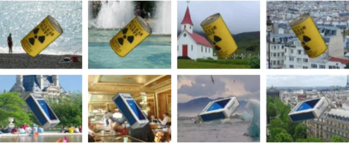
100 objects under 6 different 3D poses, inserted with a specific 2D rotation per pose on 10 backgrounds; there are 60 images per object and 10 images per 2D rotation/3D pose, as illustrated in Figure 3. DB600is obtained
by considering 20 random objects under 3 different 3D poses / 2D rotations and 10 backgrounds, leading to 30 images per object.
Figure 3: Samples of DB6000: two objects with different backgrounds and 3D poses / 2D rotations.
Visual words as labeled objects
As objects Oiused in all the evaluated techniques, we have chosen interest points in a bag-of-features
representa-tion, that attaches a category (a visual word) to each point. Points were extracted with the Harris color detector
and locally described with color differential invariants [13]; other descriptors, SIFT for example [12], could also be considered without challenging the relevance of the approach. In DB6000, the number of extracted points
varies between 300 and 600 points per image. The visual vocabulary was classically obtained using k-means as clustering algorithm [19], and its size (NL) was varied from 250 to 2000 words during the experiences.
Implementation of compared techniques
The TSR technique implemented follows work [7, 16] presented in section 1.1.1. It is applied on visual words and each key K is indexed in a B-tree. To be able to compare this approach with the semi-local version of ∆-TSR (see section 2.2.2), we have also adapted TSR to deal with a subset of all the possible triangles, and then adapted the similarity measure: this version is called TSRsl. The bag-of-features representation implemented follows the
classical one initially proposed in [19]: as associated image signature, we employ the standard weighting known as “term frequency-inverse document frequency” (tf-idf) to compute the histogram of the visual vocabulary. Each signature is indexed according to an inverted file to accelerate retrieval. Image signatures are compared with their normalized scalar product (cosine of angle). Note that a great effort was made to implement these state-of-the-art techniques optimally.
Criteria of evaluation
All the techniques are evaluated both in terms (1) of quality of the responses by computing Precision and Recall (P/R) curves (results presented in this section by displaying these curves or at least mAP, i.e. mean Average Precision for secondary results) and (2) of time retrieval by measuring CPU time and IO access (see Section 4). These measures are averaged over all the images of the tested database (DB600or DB6000) taken as queries.
Note that here, to precisely evaluate our contribution on the description of the spatial layout of visual contents, we did not end retrieval by performing a a posteriori geometric registration of the matched features to re-rank the responses, whatever the evaluated approach.
3.2
Comparison of ∆-TSR with literature
In this section, we compare ∆-TSR3D (section 2.1) to ∆-TSR5D (section 2.2.1), to TSR and to the classical
BoF representation of an image. We also evaluate its variant ∆-TSR1D that only describes co-occurrences of
objects without exploiting their geometry.
All the descriptions are built on a visual vocabulary of size NL= 1000. Because the evaluation is performed
for sub-image / object retrieval on databases of images containing 3D objects (see section 3.1), we evaluate TSR, ∆-TSR1D, ∆-TSR3D, ∆-TSR5Din their semi-local representation (strategy SL presented in section 2.2.2), noted
TSRslfor TSR. Preliminary experiments have to be done to fix the parameters associated with these approaches:
radius r of the neighborhood considered in the semi-local description of each approach, the tolerance thresholds
δa for ∆-TSR3D, δa and δo for ∆-TSR5D, Dθ for TSRsl. Table 1 reports the average precisions obtained for
optimal values of δa and Dθ with several values of r.
Whatever the approach, the best results are obtained with r = 8, and with δa = 14◦ for ∆-TSR3D and
Dθ = 1 for TSRsl. Retrieval becomes worse when the radius increases, thus demonstrating the relevance of
the semi-local representation for sub-image / object retrieval. Considering larger triangles into the description leads to an image representation less efficient because (i) less robust to viewpoint changes and (ii) involving more triplets of points overlapping object of interest and background, thus less repeatable across images. One interesting consequence of this result is that, with a small radius, the complexity of ∆-TSR3Das well as TSRsl
is notably reduced: for r = 8 on DB600, we obtain 301,091 triangles, while it is 11,300,207 when r = 32. With
TSRsl, the optimal value observed for Dθ is 1, meaning that only one class of angles is applied on angle θ. This
∆-TSR3D TSRsl r mAP δa mAP Dθ 8 0.721 14◦ 0.242 1 16 0.716 11◦ 0.229 1 24 0.683 13◦ 0.148 1 32 0.679 10◦ 0.121 1
Table 1: Evaluation of ∆-TSR3Dand TSRsl on DB600by varying radius r: mean Average Precision (mAP) for
∆-TSR3D with optimal δa for each r and for TSR with optimal Dθfor each r.
that the associated description, already illustrated in Figure 1(a), is not adapted for object retrieval with local visual features.
∆-TSR5Dis used by considering the color gaussian gradient around the point as orientation. With the best
parameters found for ∆-TSR3D (δa= 14◦, r = 8) and by varying the orientation variation interval δo, on DB600
with NL= 1000, the best results for ∆-TSR5D are obtained with δo= 27◦.
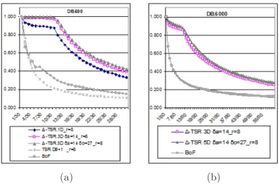
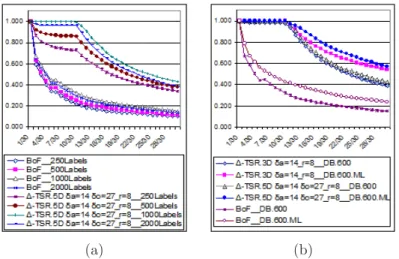
According to these results, Figure 4(a) plots the P/R curves obtained for all the approaches, with the best values of parameters r, δa, δoand Dθ, and with strategy of triangle pruning SL. These measures were computed
on DB600, comparable results were obtained on DB6000.
(a) (b)
Figure 4: Comparison of the best configuration of approaches (a) on DB600 and (b) on DB6000. First, we observe that employing ∆-TSR1Dgreatly improves retrieval with BoF only: as already studied in
works [17, 18] with doublets of visual words, characterizing the semi-local co-occurrence of objects (here with triplets of objects) produces a distinctive description of the visual content. By characterizing the geometry of triplets of objects, ∆-TSR3D brings a relevant information that increases precision even more whatever the
recall. The ∆-TSR5D description slightly enriches the ∆-TSR3D one by exploiting the object orientation. As
shown on the P/R curves of Figure 4(b), these improvements are also repeated with database DB6000, thus
confirming the usefulness of integrating the object orientation into the image signature.
Second, results obtained with TSRsl confirm that this approach is not adequate for sub-image retrieval.
In particular, choosing Dθ = 1 comes down to only considering co-occurrences of triplets, as with ∆-TSR1D.
The difference in the performance with ∆-TSR1D is due to the similarity measure associated with TSR. We
have experimented that applying our similarity measure (see Equation 12) provides a P/R curve similar to the ∆-TSR1D one.
descriptions to viewpoint changes: from recall 11/30 where viewpoint is modified, precision decreases. Indeed, viewpoint changes may lead to the disappearance/appearance of interest points that imply the modification of the set of point triplets across images.
3.3
Influence of the labels
All the experiments presented above were done with NL = 1000 and with a vocabulary built with k-means
approach as explained in Section 3.1. Here, we show how the size and the quality labels categorization can influence the quality of the ∆-TSR responses. All the experiments were done with the best configurations of all the approaches on DB600.
Influence of the vocabulary size. The vocabulary size has an effect on the discriminating power and the generalization of the signatures [23]. With a small size, the visual word features are not discriminative: dissimilar objects may be associated with the same word. As the size increases, they becomes more discriminative. In return, it becomes less generalizable and could be prone to noise such that two similar objects can be represented by different words. As shown in Figure 5(a), the influence of NL is the same for all approaches (BoF and
∆-TSR5D). From 250 to 1000 labels, the result quality increases with NL. However, after NL= 1000, the quality
decreases. Our experiments, also confirmed on DB6000, show that the best vocabulary size is 1000 labels for the
two studied approaches.
(a) (b)
Figure 5: Influence (a) of vocabulary size and (b) of vocabulary quality.
Influence of the vocabulary quality. The change on 3D pose can decrease the visual word categorization quality. Indeed, analyzing the object labels, we found that changes on 3D involve noise and then the same salient point in two images of the same object with different 3D poses can have a different label in each image. In order to improve the label quality for these experiments, we have corrected the labels by tracking the object on its trajectory through the different 3D poses. Figure 5(b) compares each approach using the original labels and the modified (corrected) labels (called ML in the figure). The result quality is improved for each approach when the labels are corrected. Moreover, the gap between ∆-T SR3Dand ∆-T SR5Dincreases with the corrected
3.4
Evaluation of ∆-PSR
As explained in Section 2.3, our approach can represent the geometrical relationships between polygons of objects. In order to evaluate the best polygon degree, we have done several experiments on database DB600
with the corrected labels. Note that the size of the polygon signature increases with the polygon degree: for example, each polygon signature is a 7-tuple when the polygon degree is 4. As shown on Figure 6, the best polygon degree is 3. The figure only shows the results obtained with ∆-4SR7D, when the polygon degree is 4.
With a higher degree, the results are worst. Indeed, the bigger the polygon degree, the bigger the signature size and the lower the probability to find similar polygons. That is why in the following experiments, we only use triangular relationships between objects.
Figure 6: Evaluation of ∆-PSR: comparison be-tween ∆-TSR5D, ∆-4SR7D and BoF on DB600.
Figure 7: P/R curves obtained with the different strategies of pruning with ∆-TSR5D on DB600.
4
Scalability of ∆-TSR
In this section, we evaluate the performances of ∆-TSR in terms of time retrieval by measuring CPU and IO times. The experiences are done with the best configurations of the methods with the real labels, determined in section 3. All the measures are averaged over all the images of the tested database (DB600 or DB6000) taken as
queries. To obtain a realistic estimation of time retrieval, measures include the computation of the description on each query image (except the step of objects extraction, i.e. interest points detection, description and categorization, which is common to all the approaches): for the image signature based on BoF, these measures include the computation of the histogram of the visual vocabulary, while they include all the relationships computation and description for TSR and ∆-TSR.
4.1
Time retrieval estimation
In order to improve time retrieval for each approach, we have developed several index structures. The best index structure for BoF representation [19] is the inverted file. In the TSR approach, because the triangle signatures are mono-dimensional, the authors use the well-known B-tree. In our approach, the triangle signatures are multidimensional and because they can be ordered according to the searching algorithm, as explained in Section 2.5, we also experimented the B-tree index with the triangle signature as the composite searching key. Nevertheless, because the signature is multidimensional, we also experimented a classical multidimensional indexing structure, the R-tree3, reputed to be efficient for range queries.
Table 2 shows the CPU and IO times of the different approaches. Using the small database DB600, the
BoF description with the inverted file is the quickest approach. Experimented on the same database, the time obtained with TSRsl and ∆-TSR is equivalent when our approach is indexed by a B-tree. Using a R-tree, we
obtained the worst times. Indeed, as explained in Section 2.4, the search process of ∆-TSR is based on a key ranking. For such kind of particular search query, the R-tree is not the optimal index structure.
DB600 DB6000
Approach / Index CPU IO CPU IO
BoF / Inverted file 85.532 6.916 292.653 26.152
TSRsl / B-tree 107.218 5.982 235.402 15.319
∆-TSR3D / B-tree 103.360 6.182 118.618 14.193
∆-TSR5D / B-tree 115.580 6.232 129.323 13.281
∆-TSR3D / R-tree 281.721 18.383 328.655 24.343
∆-TSR5D / R-tree 301.150 19.872 358.323 27.115
Table 2: CPU and IO times (in ms) of the different approaches on the 2 databases DB600 and DB6000. While CPU time is multiplied by two or three for the BoF and TSRsl approaches when using the biggest
database DB6000, it is almost constant for ∆-TSR when the index structure is a B-tree. The number of disk
accesses is multiplied by 2 for the TSRsl and ∆-TSR, while it increases more for the BoF approach. As a result,
these experiments show that the database size has a small influence on ∆-TSR.
To conclude this section, we can say that ∆-TSR really increases the quality of the results (see Section 3) with respectable execution times, compared to the other approaches.
4.2
Strategies for triangle pruning
In this section, we evaluate the relevance of the strategies proposed in section 2.2.2 for pruning triangles, in terms of time retrieval and their consequences on the quality of retrieval with ∆-TSR5D.
Evaluation of the strategies of triangle pruning. Figure 7 and Table 3 respectively present the P/R curves and time retrieval obtained when applying strategy SL, the three variants of strategy SLsemand strategy SLgeo
on DB600. In this evaluation, these strategies are both applied on the queries and the images of the database.
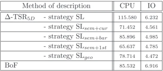
Method of description CPU IO
∆-TSR5D - strategy SL 115.580 6.232 - strategy SLsem+cur 71.452 4.561 - strategy SLsem+bar 85.896 4.985 - strategy SLsem+1st 65.637 4.785 - strategy SLgeo 78.714 4.472 BoF 85.532 6.916
Table 3: Average CPU and IO times (ms) for the 3 strategies of pruning with ∆-TSR5Don DB600. The best results in terms of quality of retrieval are obtained with strategy SL that exploits all the possible triangular relationships in the semi-local neighborhood of each object (see Figure 2 for an example). Such a redundancy in the description of the spatial relationships has the advantage of making the approach more robust to a potential bad repeatability of some points across images. But because of the amount of considered triangle signatures, this strategy is the most expensive in terms of CPU time and IO access. Immediately after, strategy SLsem+cur provides the best quality results: minimizing the amount of triangles in the description
reduces time retrieval drastically, while reducing precision of retrieval only slightly. By considering the center of the neighborhood as pivot, this strategy reduces triangles’ stretching, thus improving robustness to viewpoint changes. We observe that with the same complexity, variants SLsem+bar and strategy SLsem+1st provide the
worst precision. By considering the objects’ barycenter, SLsem+bar minimizes triangles’ stretching but is very
sensitive to the presence and geometry of any of the objects in the neighborhood, leading to the high risk of determining different pivots in corresponding neighborhoods of two images. Note that CPU time is slightly increased (around 85 ms) because of the barycenter computation in each neighborhood. By choosing the object with the first label as pivot, SLsem+1st may base the triangulation on objects that appear in several
neighborhoods, like in the example of Figure 2 with O1; the disappearance of this object has an impact on the
description of the relationships on several neighborhoods, while such a configuration is clearly less frequent with SLsem+cur. Based on a Delaunay triangulation, SLgeoprovides precision results slightly worse than SLsem+cur,
while exploiting more triangles: such a triangulation is locally sensitive to the presence/absence and geometry of objects, making it better than SLsem+bar but worse than SLsem+cur that mainly rests on labels. Because
strategies SL and SLsem+cur provide the best results, we use them in the following experiments.
Asymmetrical description of the spatial layout. In the previous experiment, the same strategy of pruning was applied both to the image queries and the database. Because in each neighborhood SLsem+cur provides a
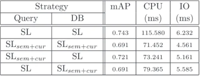
triangulation which is a subset of the one provided by SL, we also evaluate the scenario where the description of the spatial layout is done asymmetrically: query is described using a strategy different to the one used for the database. Table 4 gives the performances obtained in terms of quality and time retrieval (here, because of the paper’s size imposed, we only provide the average precision of retrieval).
Strategy mAP CPU IO
Query DB (ms) (ms)
SL SL 0.743 115.580 6.232
SLsem+cur SLsem+cur 0.691 71.452 4.561
SLsem+cur SL 0.721 73.241 5.161
SL SLsem+cur 0.691 79.365 5.585
Table 4: Performances of retrieval with ∆-TSR5D and strategies SL and SLsem+cur applied symmetrically and
asymmetrically on DB600.
We observe that scenario SLsem+cur/SL represents an interesting alternative where quality retrieval remains
very close to the best one (SL/SL), while maintaining a low complexity. Then we adopt scenarios SL/SL and SLsem+cur/SL for the last experiments that evaluate the scalability of the whole approach by increasing the
database size.
4.3
Scalability
In order to evaluate the scalability of ∆-TSR, we vary the size of the database, from 600 up to 6000 images. This evaluation is realized on NL= 1000 labels. In the image retrieval scenario, the main influence on retrieval
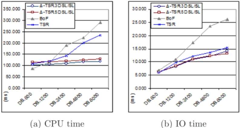
time concerns the searching technique, the computing of similarity measure and the ranking of resulting images. Figure 8 presents the execution time (CPU and IO) obtained versus the database size for BoF, TSRsl and
∆-TSR with scenario SL/SL.
With BoF and TSRsl, retrieval time increases with the database size, while ∆-TSR3Dand ∆-TSR5Dpresent
a sub-linear CPU time. Indeed, BoF spends a great part of its execution time on comparing the frequency histograms, therefore greater the visual vocabulary, greater the execution time. Moreover, for a fixed number of labels, the probability of finding images with common labels increases with the database size, and then the number of histograms to compare as well as the volume of inverted file to load from disk. TSRslassociates several
(a) CPU time (b) IO time
Figure 8: Execution time (ms) by varying the database size.
triangles to one signature while ∆-TSR provides one signature per triangle, as already stated in Section 2.1. Consequently, TSRsl presents lower filtering capacity than the ∆-TSR, increasing thus its CPU time because of
similarity computation and results ranking. In addition, the complexity of ∆-TSR similarity measure is lower than the one of TSRsl. Another consequence of such codings is that IO times for TSRsland ∆-TSR are similar
– see Figure 8(b), because despite of ∆-TSR high filtering capacity, its B-tree is larger than the one of TSRsl.
Table 5 shows statistics on the volume of features produced for the same databases: thanks to strategy of pruning SL, we see that the number of triangles vary within the same range as the number of points, while it was proved that the triangle-based description is more discriminant. Note that here, the average number of triangles per image is around 500. Consequently, with NL = 1000 (providing 1 billion of possible keys K1, see
Equation 3), in the most pessimistic configuration where all the point triplets are different, the current ∆-TSR coding can handle 2 millions of images.
# of triangles (r = 8) # of points Database in total per image in total per image
DB600 301,091 501 232,486 387
DB1200 570,542 475 453,581 377
DB2400 1,153,687 480 916,764 381
DB4800 2,790,540 581 1,565,701 326
DB6000 2,942,714 490 2,339,807 389
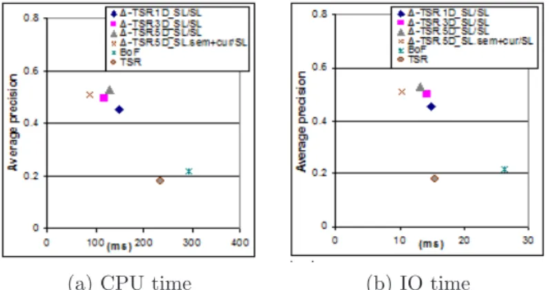
Table 5: Number of triangles and interest points in each database, and their average per image. To conclude, Figure 9 connects precision and execution times for BoF, TSRsl and the several versions of
∆-TSR on DB6000. We observe that ∆-TSR provides the best ratio precision/execution time, whatever the
variant considered.
5
Conclusions and perspectives
This paper is devoted to the representation of spatial relationships between objects in image contents. We have proposed ∆-TSR, which describes triangular spatial relationships with the aim of being invariant to image translation, rotation, scale and robust to viewpoint changes. The approach can be implemented according to 3 variants: ∆-TSR1D that describes the co-occurrence of triplets of objects, ∆-TSR3D that integrates geometry
into ∆-TSR1D by describing triplets of objects represented by their centroid, and ∆-TSR5D that improves
(a) CPU time (b) IO time
Figure 9: Ratio between mAP and execution time (ms) for several approaches and optimal strategies (SL/SL and SLsem+cur/SL) on DB6000.
image and sub-image retrieval by considering low-level visual features called visual words. We demonstrated the relevance of ∆-TSR3D and ∆-TSR5D that improve quality of retrieval notably, compared to two
state-of-the-art techniques (a visual vocabulary image representation and TSR). In addition, despite of its theoretical complexity, ∆-TSR was designed to reduce CPU time and IO access notably, by exploiting relevant strategies of triangle pruning and a B-tree as index structure. Its behavior, observed in the last experiments with databases varying from 600 to 6000 images, also demonstrated that this approach is effective and scalable.
∆-TSR was applied to low-level visual features. Perspectives of this work will consist in considering other kinds of more high-level symbolic objects, and then to propose strategies of pruning different from the current ones that may be not suited because semi-local.
References
[1] G. Bouchard and B. Triggs. Hierarchical part-based visual object categorization. In CVPR, pages I 710–715, 2005. [2] C. Chang. Spatial match retrieval of symbolic pictures. JISE, 7(3):405–422, Jan. 1991.
[3] S.-K. Chang and E. Jungert. A spatial knowledge structure for image information systems using symbolic projections. In ACM Fall Joint Computer Conference, Los Alamitos, CA, USA, pages 79–86, 1986.
[4] R. Datta, D. Joshi, J. Li, and J. Z. Wang. Image Retrieval: Ideas, Influences, and Trends of the New Age. ACM Computing Surveys, 40(2):1–60, 2008.
[5] M. J. Egenhofer and R. D. Franzosa. Point set topological relations. Intl. Journal of GIS, pages 161–174, 1991. [6] K. Grauman and T. Darrell. The pyramid match kernel: Discriminative classification with sets of image features.
In IEEE International Conference on Computer Vision, volume 2, pages 1458–1465, Beijing, China, Oct. 2005. [7] D. Guru and P. Nagabhushan. Triangular spatial relationship : a new approach for spatial knowledge representation.
Pattern Recogn. Lett., 22(9):999–1006, 2001.
[8] P. Huang and C. Lee. Image Database Design Based on 9D-SPA Representation for Spatial Relations. TKDE, 16(12):1486–1496, Dec. 2004.
[9] M. Y. Junsong Yuan, Ying Wu. Discovery of Collocation Patterns: from VisualWords to Visual Phrases. In IEEE, 2007.
[10] S. Lazebnik, C. Schmid, and J. Ponce. Beyond Bags of Features: Spatial Pyramid Matching for Recognizing Natural Scene Categories. In CVPR, pages 2169–2178, Washington, DC, USA, 2006.
[11] D. Liu, G. Hua, P. Viola, and T. Chen. Integrated Feature Selection and Higher-order Spatial Feature Extraction for Object Categorization. In CVPR, pages 1–8, 2008.
[13] P. Montesinos, V. Gouet, R. Deriche, and D. Pel´e. Matching color uncalibrated images using differential invariants. IVC Journal, 18(9):659–672, June 2000.
[14] J. C. Niebles and L. Fei-Fei. A hierarchical model of shape and appearance for human action classification. In CVPR, pages 1–8, Minneapolis, MN, 2007.
[15] J. Philbin, O. Chum, M. Isard, J. Sivic, and A. Zisserman. Object retrieval with large vocabularies and fast spatial matching. In Computer Vision and Pattern Recognition, 2007. CVPR ’07. IEEE Conference on, pages 1–8, 2007. [16] P. Punitha and D. S. Guru. Symbolic image indexing and retrieval by spatial similarity: An approach based on
B-tree. Pattern Recogn., 41(6):2068–2085, 2008.
[17] S. Savarese, J. Winn, and A. Criminisi. Discriminative Object Class Models of Appearance and Shape by Correlatons. In CVPR, pages 2033–2040, 2006.
[18] J. Sivic, B. Russell, A. Efros, A. Zisserman, and W. Freeman. Discovering objects and their location in images. In ICCV, pages 370– 377, 2005.
[19] J. Sivic and A. Zisserman. Video Google: A text retrieval approach to object matching in videos. In ICCV, pages 1470–1477, Oct. 2003.
[20] T. Tuytelaars and K. Mikolajczyk. Local invariant feature detectors: a survey. Foundations and Trends in Computer Graphics and Vision, 3(3):177–280, jan 2008.
[21] W. Wang, Y. Luo, and G. Tang. Object retrieval using configurations of salient regions. In CIVR, 2008.
[22] Z. Wu, Q. F. Ke, M. Isard, and J. Sun. Bundling features for large-scale partial-duplicate web image search. In CVPR, 2009.
[23] J. Yang, Y.-G. Jiang, A. Hauptmann, and C.-W. Ngo. Evaluating bag-of-visual-words representations in scene classification. In MIR Workshop, pages 197–206, 2007.
[24] L. Yang, P. Meer, and D. .Foran. Multiple Class Segmentation Using A Unified Framework over Mean Patches. In CVPR, pages 1–8, 2007.
[25] L. Zhu, Y. Chen, X. Ye, and A. Yuille. Structure-perceptron learning of a hierarchical log-linear model. Computer Vision and Pattern Recognition, IEEE Computer Society Conference on, 0:1–8, 2008.
[26] L. L. Zhu, Y. Chen, and A. Yuille. Learning a hierarchical deformable template for rapid deformable object parsing. IEEE Transactions on Pattern Analysis and Machine Intelligence, 99(1), 2009.