https://doi.org/10.1007/s00382-018-4596-2
Effect of empirical correction of sea-surface temperature biases
on the CRCM5-simulated climate and projected climate changes
over North America
Leticia Hernández‑Díaz1 · Oumarou Nikiéma1 · René Laprise1 · Katja Winger1 · Samuel Dandoy1
Received: 20 June 2018 / Accepted: 19 December 2018 © The Author(s) 2019
Abstract
Dynamical downscaling (DD) consists in using archives of Coupled Global Climate Models (CGCM) simulations as the atmospheric and sea-surface boundary conditions (BC) to drive nested, Regional Climate Model (RCM) simulations. Biases in the CGCM-generated driving BC, however, can have detrimental impacts on RCM performance. It is well documented for the historical period that CGCM-simulated sea-surface temperatures (SST) suffer substantial biases, especially important near coastal regions. Assuming that these SST biases are time-invariant, they could in principle be subtracted from century-long CGCM projections before being used to drive RCMs. This paper investigates the performance of a 3-step DD approach as follows. The CGCM-simulated sea-surface temperatures (SST) are first empirically corrected by subtracting their systematic biases; the corrected SST are then used as ocean surface BC for an atmosphere-only GCM (AGCM) simulation; finally this AGCM simulation provides the atmospheric lateral BC to drive an RCM simulation. This is what we refer to as the 3-step approach CGCM–AGCM–RCM of DD, which can be compared to the traditional 2-step approach CGCM–RCM consisting of driving an RCM simulation directly by CGCM-generated BC. In this paper we compare the results obtained with the two approaches, for present and future climates under RCP8.5, using the fifth-generation Canadian Regional Climate Model (CRCM5) with a grid mesh of 0.22° over the North American CORDEX domain, driven by two CMIP5 models: the Canadian Earth System Model of the Canadian Centre for Climate modelling and analysis (CanESM2) and the Earth System Model of the Max-Planck-Institut für Meteorologie (MPI-ESM-MR). The results show that, in current climate, the seasonal-mean 2-m temperature fields simulated with the 3-step DD have generally smaller biases with respect to the observations than those simulated with the 2-step DD; in fact the performance of the 3-step DD simulations often approaches that of the reanalyses-driven simulation. For the seasonal-mean precipitation field, however, the differences between the two DD methods are not conclusive. Differences between the projected climate changes with the two DD methods vary substantially depending upon the variable being considered. Differences are particularly important for temperature: over the bulk of the North American continent, the 3-step DD projects more warming in winter and less in summer. This result highlights the nonlinearities of the climate system, and constitutes an additional measure of uncertainty with DD.
Keywords Regional climate modelling · Dynamical downscaling · SST bias correction · North America · CORDEX ·
CRCM5
1 Introduction
Dynamical downscaling (DD) using fine-mesh limited-area nested regional climate models (RCMs) is one of the techniques used to generate high-resolution climate data in order to assess the anticipated climate changes at regional and local scales (Giorgi and Gutowski 2015; Rummukainen
* Leticia Hernández-Díaz [email protected]
the resulting simulated climate data is insufficient for most climate impact studies at the finer scales. However, their outputs can be used as boundary conditions (BC) to drive the higher resolution RCM simulations over selected regions of the world. The many international projects following this protocol (PRUDENCE, Christensen and Christensen 2007; ENSEMBLES; van der Linden and Mitchell 2009; NARC-CAP; Mearns et al. 2013; and CORDEX; Giorgi et al. 2009; Jones et al. 2011; Giorgi and Gutowski 2015) reflect the interest of the climate community for high-resolution simu-lated data afforded by the DD approach.
RCMs allow downscaling CGCM-simulated climate data at regional and local scales in a physically consistent man-ner. At the same time, they offer the potential for improving the CGCM-simulated data. The degree of improvement of an RCM simulation with respect to the corresponding driv-ing CGCM simulation, usually termed added value, varies depending on many factors, such as, to name just a few, the variable of interest, the type of forcing characterising a region and/or a season, the altitude of the studied phenom-enon (near surface or in the free atmosphere), the chosen statistical moment, and the spatial and temporal scales con-sidered; see for example the reviews by Feser et al. (2011) and Di Luca et al. (2015). Generally, added value is expected in regions with strong orographic forcing, land-sea contrast and for variables strongly dependent on physical processes such as precipitation. It has been shown that depending on variables, regions and season, RCMs often improve upon the CGCM driving data despite imperfections in the BC driv-ing data.
There is however a limit to what can be improved when an RCM is driven by very imperfect BC (e.g., Laprise et al. 2013). Using CGCM-generated data as BC to conduct an RCM simulation poses the problem of transmission of the errors in the imposed BC to the RCM; this is known as the “garbage in, garbage out” syndrome (e.g., Wilby and Fowler 2010; Rummukainen 2010). In fact, the driving BC has been identified as the major contributor to the uncer-tainties in regional climate projections (Déqué et al. 2007; Rowell 2006). Efforts to circumvent this issue have thus been deployed. For example, in the European projects PRU-DENCE (Christensen and Christensen 2007) and ENSEM-BLES (van der Linden and Mitchell 2009), an intermedi-ate-resolution AGCM was employed between the CGCM and RCM simulations for several GCM–RCM pairs of the experiment matrix (Déqué et al. 2014); the lower BC over the ocean of the AGCM was the observed SST to which was added the GCM-simulated climate-change (SST delta) for the future periods.
The contribution of different sources of uncertainties to climate projections depends on the region, the season
temperature and precipitation biases, but the improved atmospheric lateral BC (as a consequence of using an inter-mediate-resolution AGCM) had a large impact in reducing biases in the historical period for summer and autumn sea-sons; for the other seasons, however, results were different (Déqué et al. 2014). In a recent work over the CORDEX-Africa domain with CRCM5, Hernández-Díaz et al. (2017) found that the effect of the correction of the SST using the 3-step DD approach was very large over the Guinea Coast. Only the RCM simulations driven by the BC with corrected SST could reproduce the West African Monsoon (WAM) precipitation cycle in the region of the Guinea Coast (WA-S). On the other hand, over the CORDEX-Arctic domain, Takhsha et al. (2017) found that the correction of SST biases had much less impact for precipitation, though still positive.
As noted by Di Luca et al. (2015) and Laprise et al. (2008), the success of the DD using RCM stems from the positive balance between the gain resulting from a better representation of several phenomena with respect to the con-straints imposed by the imperfect BCs. Given the potential drawback of post-processing climate simulations to correct the biases (Maraun et al. 2017; Grenier 2018), it appears appealing to try to correct, as much as possible, the inputs of the RCM to improve their performance, thus reducing the need or the magnitude of post-processing of their outputs. The correction of CGCM-generated SST, followed by an intermediate AGCM simulation using the corrected SST as lower BC, yields improved input for the RCM simulation while keeping physical consistency between the corrected SST and the driving corresponding atmospheric variables.
In the present study we investigate the effect of applying an empirical correction of CGCM-generated SST on RCM simulations for current and future periods under RCP8.5, using the fifth-generation Canadian Regional Climate Model (CRCM5) over the CORDEX North-America domain on a grid mesh of 0.22°. Of particular interest will be to investi-gate the difference in the climate-change projections follow-ing the usual protocol of drivfollow-ing the RCM with the output of a CGCM and that obtained when the RCM is driven by the corrected SST of the CGCM.
The initial contributions to the CORDEX project over the North American domain using CRCM5 (Martynov et al. 2013; Šeparović et a. 2013) were made with a 0.44° mesh. Lucas-Picher et al. (2016) compared three reanalyses-driven CRCM5 simulations with grid meshes of 0.44°, 0.22° and 0.11° over the North American CORDEX domain. Their results showed increased added value of the RCM simulation at higher resolution: orographic precipitation, monsoonal precipitation on southwest US, snow belts around Great Lakes, wind channelling in the St. Lawrence River Valley and land-sea breezes over the Florida peninsula and the
computational costs and one must always keep in mind the ultimate goal of each experiment setup. The choice of smaller domains permitting higher resolutions at affordable cost are considered for pilot studies within the CORDEX project (Giorgi and Gutowski 2015).
Our study aims at consolidating the study of the perfor-mance of CRCM5 through the analyses of a small matrix of simulations on a 0.22° grid mesh, which is the highest resolution affordable to us for centennial simulations over the North America CORDEX domain given the available computing resources.
The paper is organised as follows. The next section pre-sents an overview of the 3-step DD approach with empirical correction of SST, the models’ description and the configu-ration of the simulations. Results for historical climate are discussed in Sect. 3 and those of climate-change projections in Sect. 4. Finally, a summary of the findings and conclu-sions are presented in Sect. 5.
2 Experiments setup
In this study, the 3-step DD approach follows the empirical correction method initially developed in Hernández-Díaz et al. (2017) and later modified in Takhsha et al. (2017). For the benefit of the reader, we summarize the 3-step DD technique in the next subsection. The models, data for vali-dation and the configuration of simulations are presented in following subsections.
2.1 The 3‑step dynamical downscaling with SST bias correction
The basic assumption of this approach is that biases in the CGCM historical simulation will persist in the future sce-nario projections; hence the SST simulated by a CGCM will be empirically corrected by subtracting the biases identified in simulating the historical period.
The notation is as follows: 𝜓G(d,m,y) corresponds to an archive of historical CGCM-simulated SST, and 𝜓A(d,m,y) is the corresponding analysed variable. Here d refers to 6-h values for each day in a month m of a year y. The historical bias is defined as:
where the −yH denotes a mean over some historical time
period yH , in this case 1979–2008. The corrected SST field
𝜓�(d,m,y) is defined as
B(d,m) = 𝜓G(d,m,y)
yH
− 𝜓A(d,m,y)
yH
Note that with this correction procedure, the instanta-neous fields 𝜓�(d
,m,y) will be rather smooth compared to reanalyses because they retain the resolution of the CGCM fields 𝜓G(d,m,y) , so they will lack fine-scale features that may be present in the analysed fields 𝜓A(d,m,y) . Also, the resulting corrected variable 𝜓�(d
,m,y) retains the CGCM-simulated temporal variability and its evolution in future time. These are the main differences with the delta method used in PRUDENCE and ENSEMBLES that benefits from the higher resolution of the analysis, but lack the future time evolution of the CGCM-simulated variability.
As in Takhsha et al. (2017), the empirical correction is here restricted to the SST field due to the challenge of correcting both SST and sea-ice concentration (SIC) while keeping the physical consistency between these variables for the future under global warming. For the current work, the CGCM-simulated SIC is used without adjustment, and the corrected SST is modified when required to ensure consist-ency between the SIC and SST fields.
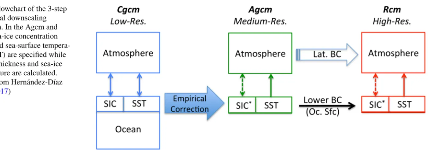
Clearly the adjusted SST field is inconsistent with the CGCM-simulated atmospheric fields, and hence it would be inappropriate to use the CGCM-simulated fields as lat-eral atmospheric BC to drive an RCM simulation. Hence a second step is added that consists in running an atmosphere-only GCM (AGCM) using the corrected SST as ocean sur-face BC. The third and final step is to use the atmospheric fields from the AGCM simulation, together with the cor-rected SST, as lateral atmospheric BC and surface ocean BC, respectively, for driving an RCM simulation over the region of interest: in the present case, the North American CORDEX domain. Figure 1 shows a flowchart describing the 3-step dynamical downscaling technique.
2.2 Models
The RCM employed in this study is the fifth-generation Canadian Regional Climate Model (CRCM5; Hernández-Díaz et al. 2013; Martynov et al. 2013). In a nutshell, CRCM5 is based on a limited-area configuration of the Global Environment Multiscale (GEM) model (Bélair et al. 2005, 2009) employed for numerical weather predic-tion by the Canadian Meteorological Centre (CMC). The subgrid-scale physical parameterisations include the Kain and Fritsch (1990) deep-convection and Kuo-transient (Kuo 1965) shallow-convection schemes, as well as the Sundqvist et al. (1989) large-scale condensation scheme, the corre-lated-K scheme for solar and terrestrial radiations (Li and Barker 2005), a subgrid-scale mountain gravity-wave drag (McFarlane 1987) and low-level orographic blocking (Zadra et al. 2003), a turbulent kinetic energy closure in the
plan-changed from ISBA used at CMC for the Canadian LAnd Surface Scheme (CLASS; Verseghy 2000, 2008) in its most recent version, CLASS 3.5. For these simulations, 26 soil layers are used, reaching to a depth of 60 m. The standard CLASS distributions of sand and clay fields as well as the bare soil albedo values are replaced by data from the ECO-CLIMAP database (Masson et al. 2003). Finally, the interac-tive thermo-dynamical 1-D lake module (FLake model) is also used (see Martynov et al. 2010, 2012).
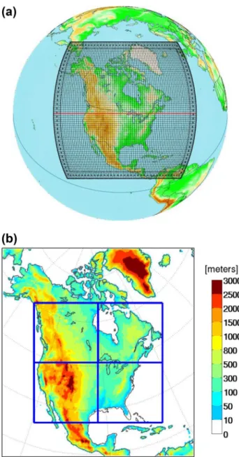
The CRCM5 was integrated over the North American CORDEX domain (Fig. 2) with a grid mesh of 0.22°, with a 10-min timestep. The free domain has 340 × 320 grid points, excluding the 10-grid-point wide sponge zone and the 10-grid-point wide semi-Lagrangian halo around the perimeter. In the vertical, 56 levels were used, with the top level near 10 hPa and the lowest level at 0.996*ps where ps
is the surface pressure. For diagnostic analysis most vari-ables were archived at 3 h intervals, except precipitation and surface fluxes that were cumulated and archived at hourly intervals.
The AGCM used in this study is a global version of CRCM5, with a regular latitude-longitude grid of 1° and 64 levels in the vertical, with a top level at 2 hPa, and a timestep of 45 min. Given that the AGCM does not involve coupling with an ocean, an intermediate resolution between that of the RCM and the CGCM could be afforded, which also possibly contributes to improving the lateral BC driving the RCM. Subgrid-scale physical parameterisations are the same of those of CRCM5, except for small differences in convection-related formulation to account for differences in resolution. The two CGCMs used as driving data are CanESM2 and MPI-ESM-MR, both from the CMIP5 database. CanESM2 (Arora et al. 2011) has its atmospheric component oper-ating at T63 with a linear transform grid of 2.81° and 35 vertical levels, whereas the ocean component has horizon-tal grid spacing of 1.41° in longitude and 0.94° in latitude.
MPI-ESM-MR (https ://verc.enes.org/model s/earth syste m-model s/mpi-m/mpi-esm) has its atmospheric component is operating at T63, with a linear transform grid of approxi-mately 2.85° and 95 levels in the vertical, whereas its ocean component operates at 0.4° and has 40 vertical levels. Fig-ure 3 shows the climatological SST biases of CanESM2 and MPI-ESM-MR (hereinafter referred to as Cgcm1 and Cgcm2, respectively) with respect to ERA-Interim reanaly-ses (Dee et al. 2011) for the period 1981–2010; we note the particularly large biases near the coastal regions that the empirical correction aims at removing.
2.3 Observational data
The CRCM5 simulations will be compared to climate research unit (CRU) gridded analysis of observations data-set (version 3.21, from 1901 to 2012; Harris et al. 2014) on a 0.5° grid with monthly temporal resolution.
2.4 Simulations configuration
The CanESM2 and MPI-ESM-MR archives cover the period 1949–2100, under historical and RCP8.5 emission scenario. The period 1979–2008 was chosen to calculate the SST biases with respect to ERA-Interim reanalyses. The corrected SST fields are then used as ocean surface BC for 2 AGCM simulations (referred to as Agcm_e1 and Agcm_e2, the subscript e being used as a reminder of the empirical correction applied to CGCM-simulated SST fields and the numbers as indicators of the corresponding CGCM outputs), from 1949–2100 under historical and RCP8.5 emission scenario. Finally, the Agcm_e# simulations will provide the atmospheric lateral BC for the CRCM5 simula-tions over the North American CORDEX domain for the same period (1949–2100), using the corrected SST fields; these simulations will be referred to as Rcm/Agcm_e1 and
Fig. 1 Flowchart of the 3-step dynamical downscaling approach. In the Agcm and Rcm, sea-ice concentration (SIC) and sea-surface tempera-ture (SST) are specified while sea-ice thickness and sea-ice temperature are calculated. Taken from Hernández-Díaz et al. (2017)
Rcm/Agcm_e2, and they will be compared to those driven by the corresponding CGCM-driven CRCM5 simulations following the usual two-step dynamical downscaling, noted as Rcm/Cgcm1 and Rcm/Cgcm2.
In addition to these simulations for the 1949–2100 time period, a reanalysis-driven hindcast simulation (Rcm/ReAn) has also been performed for the 1979–2010 time period,
European Centre for Medium-range Weather Forecasting (ECMWF) ERA-Interim reanalyses (Dee et al. 2011) avail-able to us on a 0.75° horizontal grid. In summary, for this study a total of 2 AGCM simulations and 5 RCM simulations have been carried out as shown in Table 1, in addition to the 2 CGCM simulation archives taken from the CMIP5 database.
3 Historical climate simulations
In this section the skill of the 3-step DD (Rcm/Agcm_e1 and Rcm/Agcm_e2) and 2-step DD (Rcm/Cgcm1 and Rcm/ Cgcm2) CRCM5 historical simulations are assessed with respect to the CRU reference observational dataset, and compared to the ERA-driven hindcast simulation (Rcm/ ReAn). Figure 2b shows the four quadrants over which the RMS difference between the CRM5 simulations and CRU will be computed over land points to objectivize the com-parison of the two DD methods. The RMS values computed over the four quadrants, are given in Table 2, for temperature and precipitation, for winter and summer.
3.1 Seasonal mean climatology of 2‑m temperature
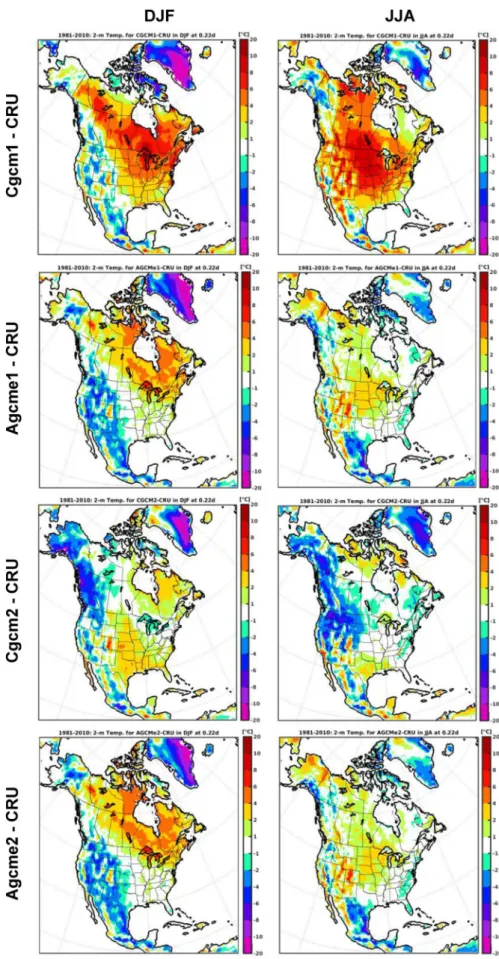
Figure 4 shows the climatological 2-m temperature biases of the Rcm/Cgcm#, Rcm/Agcm_e# and Rcm/ReAn simula-tions relative to CRU for the period 1981–2010, in boreal winter (DJF) and boreal summer (JJA). The large winter temperature bias over the Great Lakes indicates the limita-tion of the 1-D lake model used in CRCM5. The last row in Fig. 4 shows the difference between the Rcm/Cgcm# and Rcm/Agcm_e# historical simulations to illustrate the impact of the 3-step DD with empirical correction of SST. The sim-ulations using the archive of the Cgcm1 are in Fig. 4a and the simulations using the archive of the Cgcm2 in Fig. 4b.
In winter, the Rcm/Cgcm1 exhibits a strong cold bias over the southwest part of the continent and a strong warm bias over the northeast region (Fig. 4a); the bias over the SW quadrant is reduced by 45% in Rcm/Agcm_e1 (Table 2). In summer, there is a strong warm bias over most part of the continent, with the largest values over Western Canada; this warm bias is reduced by 74% in the Rcm/Agcm_e1 simula-tion (Table 2). It is worth noting that the Rcm/Cgcm1 warm biases are inherited from the driving model Cgcm1, as can be seen in Fig. 5 (1st row).
The temperature improvement of the Rcm/Agcm_e1 with respect to the Rcm/Cgcm1 is remarkable, but some points are worth to be noted. Comparing these results to the hindcast simulation (Rcm/ReAn) biases (Fig. 4a, 3rd row) allows us to see that, while the skill of the Rcm/Agcm_e1 is
Fig. 2 a CORDEX North-America domain for the 0.22° CRCM5 simulation, including the 10 grid-point semi-Lagrangian halo and the 10 grid-point Davies sponge zone; only every 10th grid boxes are dis-played. b The CRCM5 topography and the four quadrants over which the RMS difference between the CRCM5 simulation and the refer-ence observational field will be computed over land points
that of the reference simulation (Rcm/ReAn) in DJF. On the other hand, in JJA the Rcm/Agcm_e1 is overall better than the reference simulation (Rcm/ReAn), which is indicative of compensation between structural errors of CRCM5 and errors inherited from BC forcing. Overall the 3step DD sim-ulation is substantially better than the 2-step DD simsim-ulation for temperature (see Table 2), and differences between the two are important, as can be seen in the last row of Fig. 4a.
Figure 4b presents corresponding results obtained with the Cgcm2 archive. In winter, the Rcm/Cgcm2 cold bias over the western half of the continent is much reduced in Rcm/ Agcm_e2 (a reduction by 12% of the RMS over the SW quad-rant; see Table 2), but this is at the expense of an increased warm bias in most of eastern Canada (an increase by 94% and
27% of the RMS over the NE and SE quadrants, respectively; see Table 2). We note that this warm bias is also present in the driving model Agcm_e2 (see Fig. 5, 4th row). In summer, much of the cold bias present in the 2-step DD simulation is eliminated in the 3-step DD simulation, except over Mexico, without negative repercussions in this case; RMS reductions range between 13 and 46% depending upon the quadrants (see Table 2). In JJA both 3-step DD simulations Rcm/Agcm_e1 and Rcm/Agcm_e2 exhibit superior performance than that of the hindcast simulation Rcm/ReAn; this counterintuitive result is assuredly indicative of compensation between struc-tural errors of the RCM and of that of the driving BC.
A visual analysis of Figs. 4 and 5 also tells us that for current climate, although the 2-step DD simulations have
Fig. 3 Sea surface temperature (SST) bias of the Cgcm1 (1st row) and Cgcm2 (2nd row) with respect to ERA-Interim reanalyses, for boreal win-ter (left column) and summer (right column), for the period 1981–2010
Table 1 Matrix of simulations carried out in this study
Two AGCM simulations have been done to serve as lateral BC to drive the RCM: one using the empirically corrected CGCM1 SST (Agcm_e1) and one using the empirically corrected CGCM2 SST (Agcm_e2). Five RCM simulations have been done: a reanalyses-driven RCM simulation (Rcm/ReAn), two CGCM-driven RCM simulations (Rcm/Cgcm1 and Rcm/Cgcm2), and two AGCM-driven RCM simulations (Rcm/Agcm_ e1 and Rcm/Agcm_e2) at 0.22°. All but Rcm/ReAn simulations were performed for the 1949–2100 time period; Rcm/ReAn was performed for the period 1979 to 2010
Global simulations
AGCM: CRCM5 global version
Name Ocean surface BC
Agcm_e1 Bias-corrected Can_ESM2 SST
Agcm_e2 Bias-corrected MPI-ESM-MR SST
Regional simulations
RCM: CRCM5 regional version
Name Atmospheric lateral BC Ocean surface BC
Rcm/ReAn ERA-I Reanalyses ERA-I Reanalyses
Rcm/Cgcm1 Can_ESM2 Can_ESM2
Rcm/Agcm_e1 CRCM5 global version Bias-corrected Can_ESM2 SST
Rcm/Cgcm2 MPI-ESM-MR MPI-ESM-MR
Rcm/Agcm_e2 CRCM5 global version Bias-corrected MPI-ESM-MR SST
Table 2 RMS differences of Rcm/Cgcm# and Rcm/Agcm_e# simulated results with respect to the CRU reference dataset, and the percent difference between the two RMS values, for # = 1 and 2
The RMS differences are computed over the 4 quadrants (NW, SW, NE and SE) shown in Fig. 2b, for the fields of 2-m temperature and precipitation, in winter (DJF) and summer (JJA). Percent differences values exceeding ± 10% are shaded in orange and green, respectively
Fig. 4 a 2-m temperature bias for 1981–2010 compared to observational dataset CRU (available over land), for the historical simulations Rcm/ Cgcm1 (1st row) and Rcm/ Agcm_e1 (2nd row) and for the hindcast simulation Rcm/ReAn (3rd row). The 4th row shows the difference between the Rcm/ Cgcm1 and Rcm/Agcm_e1 historical simulations. b 2-m temperature bias for 1981–2010 compared to observational data-set CRU (available over land), for the historical simulations Rcm/Cgcm2 (1st row) and Rcm/ Agcm_e2 (2nd row) and for the hindcast simulation Rcm/ReAn (3rd row). The 4th row shows the difference between the Rcm/ Cgcm2 and Rcm/Agcm_e2 historical simulations
Fig. 5 2-m temperature bias for 1981–2010 compared to obser-vational dataset CRU (avail-able over land), for the driving models historical simulations Cgcm# (1st and 3rd row) and Agcm_e# (2nd and 4th row)
Fig. 6 2-m temperature bias for 1981–2010 compared to the reference simulation (Rcm/ ReAn), for the historical simula-tions Rcm/Cgcm# (1st and 3rd row) and Rcm/Agcm_e# (2nd and 4th row)
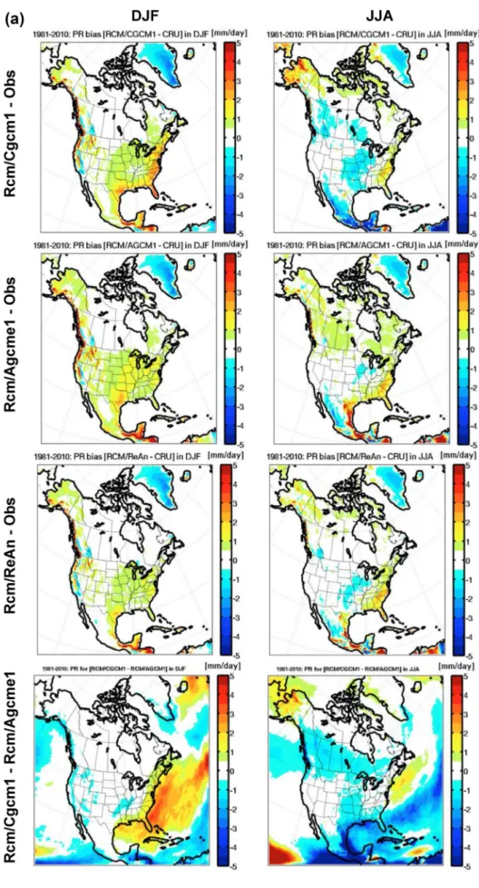
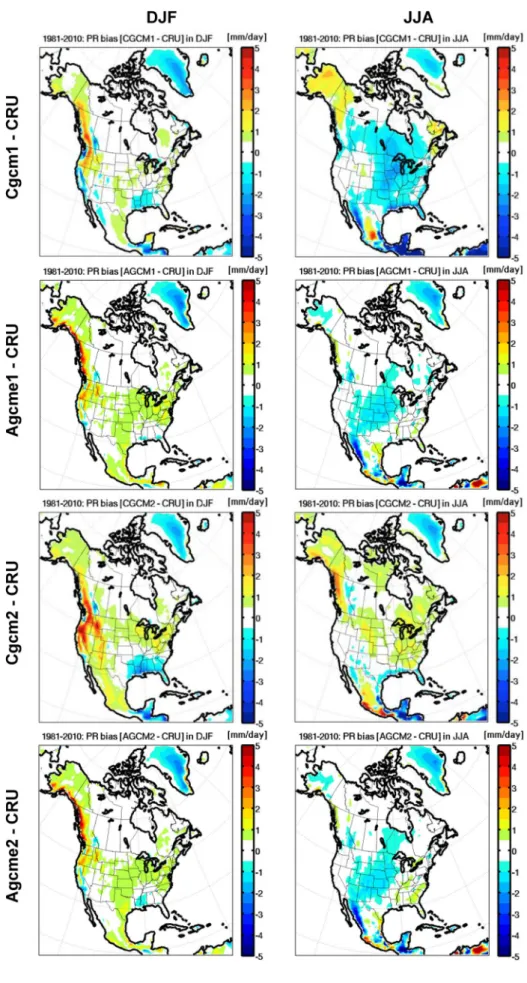
Fig. 7 a Precipitation bias (mm/ day) for 1981–2010 compared to observational dataset CRU (available over land), for the historical simulations Rcm/ Cgcm1 (1st row) and Rcm/ Agcm_e1 (2nd row) and for the hindcast simulation Rcm/ ReAn (3rd row). The 4th row shows the difference between the Rcm/Cgcm1 and Rcm/ Agcm_e1 historical simula-tions. b Precipitation bias (mm/ day) for 1981–2010 compared to observational dataset CRU (available over land), for the historical simulations Rcm/ Cgcm2 (1st row) and Rcm/ Agcm_e2 (2nd row) and for the hindcast simulation Rcm/ReAn (3rd row). The 4th row shows the difference between the Rcm/ Cgcm2 and Rcm/Agcm_e2 historical simulations
Fig. 8 Precipitation bias (mm/ day) for 1981–2010 compared to observational dataset CRU (available over land), for the driving models historical simu-lations Cgcm# (1st and 3rd row) and Agcm_e# (2nd and 4th row)
Fig. 9 Precipitation bias (mm/ day) for 1981–2010 compared to the reference simulation (Rcm/ReAn), for the his-torical simulations Rcm/Cgcm# (1st and 3rd row) and Rcm/ Agcm_e# (2nd and 4th row)
different performance when compared to the observations, as do their driving Cgcm, the corresponding 3-step DD sim-ulations have a very similar skill. Table 2 shows that Rcm/ Agcm_e1 and Rcm/Agcm_e2 have similar RMS temperature differences, for summer and winter, and over the four quad-rants. This implies that the driving models differences are strongly transmitted in the 2-step DD case, while the differ-ences are much weakened once the intermediate step with the Agcm_e# is performed. As we shall see later however, even if the Rcm/Agcm_e1 and Rcm/Agcm_e2 simulations are very similar under present conditions, the correspond-ing projected climate changes will be significantly different. A comparison of the DD simulations to the hindcast simulation (Fig. 6) shows that the 3-step DD simulations are usually closer to the reference simulation (Rcm/ReAn) than the 2-step ones. The exception is the case of Rcm/ Agcm_e2 in DJF, which seems to stem from the fact that the driving Agcm_e2 data exhibits larger biases than Cgcm2 (Fig. 5).
3.2 Seasonal mean climatology of precipitation
The precipitation biases of the Rcm/Cgcm#, Rcm/Agcm_e# and Rcm/ReAn simulations compared to CRU gridded anal-ysis of observations over land for the period 1981–2010, in boreal winter (DJF) and boreal summer (JJA), are pre-sented in Fig. 7 (1st row–3rd row). The 4th row shows the difference between the Rcm/Cgcm# and Rcm/Agcm_e# historical simulations to illustrate the impact of the 3-step DD. The simulations using the archive of the Cgcm1 are in Fig. 7a and the simulations using the archive of the Cgcm2 in Fig. 7b.
In winter, the suite of simulations corresponding to the Cgcm1 (Fig. 7a) indicates that precipitation biases of the 3-step DD simulation (Rcm/Agcme1) are smaller compared to those of the 2-step DD simulation (Rcm/Cgcm1) in the East, but larger in the West (reduction of RMS of 2% and 42% in the NE and SE quadrants, respectively, and increase of RMS of 22% and 33% in the SW and NW quadrants,
respectively; see Table 2). In summer, the biases of 3-step DD simulation are generally larger than those of the 2-step DD simulation (RMS increase varying between 0 and 40%; see Table 2). The largest precipitation differences between the two DD methods are found over the ocean, and around the rim of the Gulf of Mexico in summer (last row in Fig. 7a).
Regarding the simulations corresponding to the Cgcm2 (Fig. 7b), biases in summer diminish going from the 2-step DD simulation to the 3-step DD simulation; RMS differ-ences are reduced between 10 and 20% for all diagnostic quadrants except the SE that increases by 2% (see Table 2). Precipitation biases in winter however vary depending upon the diagnostic quadrants; compared to the 2-step DD, the 3-step DD reduces the bias over the southwestern quadrant but increases it over the northeastern one. The last row of the figure shows that the differences in simulated precipitation between the two approaches of DD are mostly found over the oceans.
Comparing the first and second rows of Fig. 7a, b, it can be seen that while the biases in simulated precipitation of the two Rcm/Cgcm# simulations are rather different, those of the corresponding Rcm/Agcm_e# simulations are very similar; this is also confirmed in Table 2. Figure 8 shows that this is also the case for the driving models Cgcm# and Agcm_e#, namely that while Cgcm1 and Cgcm2 precipitation biases are very different, the Agcm_e1 and Agcm_e2 precipitation biases are very similar. Compar-ing Figs. 7 and 8, we see that the downscaled results in general exhibit bias of the same order of magnitude as the driving simulation; a noteworthy exception is in sum-mer with Cgcm1 in which case the downscaled results are clearly better. Over the eastern half of the North American continent in winter, Cgcm1 and Cgcm2 exhibit smaller precipitation biases than its corresponding driven simu-lations (Rcm/Cgcm1 and Rcm/Cgcm2); the same occurs for the Agcm_e1 and Agcm_e2 simulations and the cor-responding driven simulations (Rcm/Agcm_e1 and Rcm/ Agcm_e2). This may result from a tendency of nested models to amplify some of the biases of the driving data; this illustrates the challenges of putting in evidence the added value of Rcm simulations with respect to their driv-ing models. It is important to keep in mind however that the CRU dataset used as reference has rather coarse reso-lution, which prevents assessing the added value of higher resolution DD results over mountains. Lucas-Picher et al. (2016) have also shown that the main added value from high-resolution dynamical downscaling is not to be found in the large-scale fields but rather in a better depiction of finer scale, local processes.
Fig. 10 a Projected changes (2071–2100)–(1981–2010) for DJF 2-m temperature (°C) by Cgcm1, Rcm/Cgcm1 and Rcm/Agcm_e1 (first row) and Cgcm2, Rcm/Cgcm2 and Rcm/Agcm_e2 (third row). The second and fourth rows show the difference of projected cli-mate changes between the Cgcm and the Rcm/Cgcm (left) as well as between the Rcm/Cgcm and the Rcm/Agcm_e (right). b Projected changes (2071–2100)–(1981–2010) for JJA 2-m temperature (°C) by Cgcm1, Rcm/Cgcm1 and Rcm/Agcm_e1 (first row) and Cgcm2, Rcm/Cgcm2 and Rcm/Agcm_e2 (third row). The second and fourth rows show the difference of projected climate changes between the Cgcm and the Rcm/Cgcm (left) as well as between the Rcm/Cgcm and the Rcm/Agcm_e (right)
Finally, Fig. 9 shows that the 3-step DD simulation is systematically closer to the reference simulation Rcm/ReAn than the 2-step DD simulation, and this is valid for the two models, Cgcm1 and Cgcm2.
4 Climate‑change projections
In this section we analyse the effect of the 3-step DD on the projected climate changes in seasonal-mean 2-m temperature and precipitation.
Figure 10 shows the projected 2-m temperature changes for the end of the twenty-first century (2071–2100) com-pared to the reference period (1981–2010), for (a) DJF and (b) JJA. The first two rows show the suite of simulations related to Cgcm1 and Agcm_e1, while the last two rows the suite of simulations related to Cgcm2 and Agcm_e2. Rows 1 and 3 show the projected change from the Cgcm# as well as from the Rcm following the 2-step (Rcm/Cgcm#) and 3step (Rcm/Agcm_e#) DD technique. This is followed (rows 2 and 4, left panel) by the difference of the projected climate change between the driving Cgcm# and the Cgcm#-driven Rcm. Differences between the projected climate changes from the 2-step (Rcm/Cgcm#) and 3-step (Rcm/ Agcm_e#) DD technique are shown in the right panel of rows 2 and 4.
For both seasons, and without surprise, the simulated climate becomes warmer at the end of the century, the warming in the DJF season being much larger than that in JJA over the northern regions. Also, the warming pro-jected by the Cgcm1 is stronger than that propro-jected by the Cgcm2. In DJF, the warming in the Rcm/Cgcm1 and Rcm/Cgcm2 simulations is similar to that of the driving Cgcm1 and Cgcm2 simulations, although there seems to be a slight tendency to reduced warming in several regions. The Rcm/Agcm_e1 and Rcm/Agcm_e2 projected climate changes for 2-m temperature are very different from the corresponding 2-step DD projected change. In winter the 2-step DD projected warming is smaller than that of the 3-step DD over a large portion of the continent; in JJA, on the contrary, the 2-step DD projected warm-ing is stronger than that of the 3-step DD, the difference being most pronounced in the case of Rcm/Cgcm1 and Rcm/Agcm_e1.
It is interesting to note that, while there was a great similarity between the Rcm/Agcme1 and Rcm/ Agcme2 simulated 2-m temperature in current climate (1981–2010), the corresponding projected climate changes are very different. The projected climate changes in 2-m temperature for the two 3-step DD simulations
are very different, particularly in JJA (see the last panels of rows 1 and 3 in Fig. 10a, b). This can be explained by the fact that the Agcm_e# retains the SST variability and warming trend of the parent Cgcm#, which are quite dif-ferent between the two Cgcm#.
Another interesting point is that the differences between the projected climate change using the two methods of DD are of the same order as the differences between the two 2-step DD simulations as well as between the two Cgcm# and the two Agcm_e# themselves; this we take as indicative of the uncertainty in the projection of climate changes.
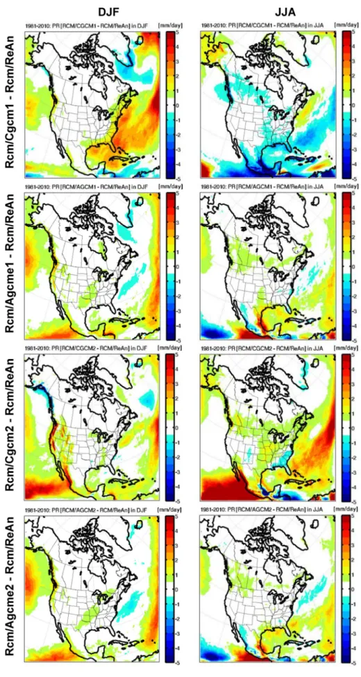
The projected changes in seasonal-mean precipitation for the end of the century (2071–2100) with respect to the reference period (1981–2010) are shown in Fig. 11 follow-ing the same order of Fig. 10. The changes in seasonal-mean precipitation projected by the two Cgcm# exhibit consistent large-scale characteristics of reduced precipita-tion at lower latitudes and enhanced precipitaprecipita-tion at higher latitudes; but the geographical details of changes are rather different (see left panels of rows 1 and 3). The Cgcm1 shows an increase in precipitation of a higher magnitude and geographical extension than Cgcm2, and located in a different region; for example, the southeast portion of North America has a different projection of precipitation changes following each model. The corresponding 2-step DD simulations (Rcm/Cgcm1 and Rcm/Cgcm2) repro-duce similar patterns to their driving models, with some enhancement of the intensities particularly over the ocean, but over the continent the driven and driving models are very similar (see left panel of second and fourth rows). On the other hand, the projected changes of the 3-step DD simulations are quite different from the corresponding 2-step ones, the difference being larger in the case of Rcm/ Cgcm1 and Rcm/Agcme_e1 (right panel, second row). Note also that the 3-step DD simulations (Rcm/Agcm_e1 and Rcm/Agcm_e2) give different projections of seasonal mean precipitation while having the same AGCM model, but different SSTs (right panels, first and third rows); the projected precipitation differences between the 2-step and 3-step DD simulations are generally larger for the Cgcm1 suite of models.
In summer (Fig. 11b), Cgcm1 and Cgcm2 both project a reduction of precipitation in the Caribbean area, but entirely different changes in the southwest corner of the displayed domain. The 2-step DD simulations (Rcm/Cgcm1 and Rcm/ Cgcm2) inherit overall the change pattern of their driving models, with some modulation in intensities; the difference Cgcm1–Rcm/Cgcm1 is larger than that of Cgcm2–Rcm/ Cgcm2. The increase of precipitation projected by Cgcm1
in the southwest USA is absent in Rcm/Cgcm1 as well as in Rcm/Agcm_e1. The increase of precipitation in Alaska projected by Cgcm1 is also found in Rcm/Cgcm1 but disap-pear in Rcm/Agcm_e1; the same is found with the Cgcm2, Rcm/Cgcm2 and Rcm/Agcm_e2 suite. At the same time, the reduction in precipitation projected in the central part of the domain by Rcm/Cgcm1 is quasi inexistent in Rcm/ Agcm_e1.
On the other side, the projected increase in precipitation of Cgcm2 in the southeast of USA is not present in Rcm/ Cgcm2, neither in Rcm/Agcm_e2; the Florida peninsula is, on the contrary, dryer in Rcm/Agcm_e2, as was the case in Cgcm1, Rcm/Cgcm1 and Rcm/Agcm_e1. In summer, the two 3-step DD simulations project similar precipitation changes over the continent.
The differences between the Rcm/Cgcm# and Rcm/ Agcm_e# precipitation changes for 2071–2100 shown in the second and fourth rows (right panel) are smaller than the corresponding ones for the historical period 1981–2010 seen in the last rows in Fig. 7a, b, yet not negligible. As said previously, this can be regarded as part of the uncertainties in climate projections.
5 Conclusions
In this paper we analysed climate simulations performed by CRCM5 on a 0.22° grid mesh over the CORDEX North America domain under historical and RCP8.5 future sce-nario, using two CMIP5 CGCM: CanESM2 and MPI-ESM-MR. Besides the usual dynamical downscaling approach (2-step DD) in which the RCM is driven by the archive of the driving CGCM, we applied the 3-step DD technique, following the work of Hernández-Díaz et al. (2017) over Africa and Takhsha et al. (2017) over the Arctic, with an empirical correction of the CGCM-simulated SST, followed
by an intermediate step of an atmosphere-only AGCM simu-lation. The objective of the exercise was to see the impact of correcting systematic SST biases on the simulated climates, for the past and the future.
For current climate, the 3-step DD simulations (Rcm/ Agcm_e1 and Rcm/Agcm_e2) have in general smaller seasonal-mean temperature biases with respect to the CRU analysis of observations than the 2-step DD simulations; the biases in fact approach those of the reanalyses-driven simulation (RCM/ReAn). For seasonal-mean precipitation the differences between the two methods of DD is mixed, ranging from a reduction of RMS precipitation bias of 40% to an increase of 42%, depending upon the GCM, season, and diagnostic quadrant.
Projected climate changes for the end of the century under RCP8.5 are also different for the two DD meth-ods: over a large part of North America, the 3-step DD projections indicate more warming in winter and less warming in summer with respect to the 2-step DD pro-jections. Regarding the seasonal-mean precipitation, the 3-step DD projections show higher intensities and more extended regions of increased precipitation over the conti-nent in winter and less precipitation in summer, compared to the 2-step DD projections. Differences in projected climate change between the two methods of DD are, at least, as important as the differences between the driving and driven model of the 2-step DD simulations and often larger; this is the situation for the two studied variables in the two seasons and the two CGCM models and their suite of simulations.
Another point to note is the great similarity of the sim-ulated 2-m temperature in current climate (1981–2010) between Rcm/Agcm_e1 and Rcm/Agcm_e2, but the rather different projected climate changes. Though they share the same intermediate AGCM model, the corrected SST from their respective CGCM keeps the CGCM-simulated variability and warming trend, which is different from one CGCM to the other. So, similar current climate simulated by the two 3-step DD does not give similar future climate change. In the case of precipitation, 3-step DD simula-tions are also rather similar in both seasons for the period of current climate, but different in the future, the differ-ence in the future being more important in winter than in summer.
The differences in climate changes projected by the two DD approaches (with and without empirical correction of SST biases) are another indication of the uncertainties in downscaled climate simulations.
Fig. 11 a Projected changes (2071–2100)–(1981–2010) for DJF pre-cipitation (mm/day) by Cgcm1, Rcm/Cgcm1 and Rcm/Agcm_e1 (first row) and Cgcm2, Rcm/Cgcm2 and Rcm/Agcm_e2 (third row). The second and fourth rows show the difference of projected cli-mate changes between the Cgcm and the Rcm/Cgcm (left) as well as between the Rcm/Cgcm and the Rcm/Agcm_e (right). b Projected changes (2071–2100)–(1981–2010) for JJA precipitation (mm/day) by Cgcm1, Rcm/Cgcm1 and Rcm/Agcm_e1 (first row) and Cgcm2, Rcm/Cgcm2 and Rcm/Agcm_e2 (third row). The second and fourth rows show the difference of projected climate changes between the Cgcm and the Rcm/Cgcm (left) as well as between the Rcm/Cgcm and the Rcm/Agcm_e (right)
Acknowledgements This research was funded in part by the follow-ing grants: the project “Marine Environmental Observation, Predic-tion and Response” (MEOPAR; http://meopa r.ca) of the Networks of Centres of Excellence (NCE; http://www.nce-rce.gc.ca) of Canada, the Discovery Accelerator Supplements Program (http://www.nserc -crsng .gc.ca/Profe ssors -Profe sseur s/Grant s-Subs/DGAS-SGSA_eng. asp) of the Natural Sciences and Engineering Research Council of Canada (NSERC; http://www.nserc -crsng .gc.ca), the Canadian Net-work for Regional Climate and Weather Processes (CNRCWP; http:// www.cnrcw p.uqam.ca) funded by the NSERC Climate Change and Atmospheric Research (CCAR; http://www.nserc -crsng .gc.ca/Profe ssors -Profe sseur s/Grant s-Subs/CCAR-RCCA_eng.asp) program. Computations were made on the supercomputer Guillimin of Cal-cul Québec-Compute Canada (http://www.calcu lqueb ec.ca) whose operation is funded by the Canada Foundation for Innovation (CFI), NanoQuébec, RMGA and the Fonds de recherche du Québec-Nature
et technologies (FRQ-NT). The authors thank Mr Georges Huard and
Mrs Nadjet Labassi for maintaining an efficient and user-friendly local computing facility. This study would not have been possible without the access to valuable data such as ERA-Interim and CRU, as well as outputs from the CMIP5 database, in this case the MPI-ESM-MR and CanESM2 models output.
Open Access This article is distributed under the terms of the Crea-tive Commons Attribution 4.0 International License (http://creat iveco mmons .org/licen ses/by/4.0/), which permits unrestricted use, distribu-tion, and reproduction in any medium, provided you give appropriate credit to the original author(s) and the source, provide a link to the Creative Commons license, and indicate if changes were made.
References
Arora VK, Scinocca JF, Boer GJ, Christian JR, Denman KL, Flato GM, Kharin VV, Lee WG, Merryfield WJ (2011) Carbon emis-sion limits required to satisfy future representative pathways of greenhouse gases. Geophys Res Lett 38:L05805
Bélair S, Mailhot J, Girard C, Vaillancourt P (2005) Boundary-layer and shallow cumulus clouds in a medium-range forecast of a large-scale weather system. Mon Weather Rev 133:1938–1960 Bélair S, Roch M, Leduc AM, Vaillancourt PA, Laroche S, Mailhot J
(2009) Medium-range quantitative precipitation forecasts from Canada’s New 33-km deterministic global operational system. Weather Forecast 24:690–708. https ://doi.org/10.1175/2008W AF222 2175.1
Benoit R, Côté J, Mailhot J (1989) Inclusion of a TKE boundary layer parameterization in the Canadian regional finite-element model. Mon Weather Rev 117:1726–1750
Christensen JH, Christensen OB (2007) A summary of the PRU-DENCE model projections of changes in European climate by the end of this century. Clim Change 81:7–30. https ://doi. org/10.1007/s1058 4-006-9210-7
Dee DP, Uppala SM, Simmons AJ, Berrisford P, Poli P, Kobayashi S, Andrae U, Balmaseda MA, Balsamo G, Bauer P, Bechtold P, Beljaars ACM, van de Berg L, Bidlot J, Bormann N, Delsol C, Dragani R, Fuentes M, Geer AJ, Haimberger L, Healy SB, Hers-bach H, Holm EV, Isaksen L, Kallberg P, Kohler M, Matricardi M, McNally AP, Monge-Sanz BM, Morcrette J-J, Park B-K, Peubey C, de Rosnay P, Tavolato C, Thepaut J-N, Vitart F (2011) The ERA-Interim reanalysis: configuration and performance of the data assimilation system. QJR Meteorol Soc 137:553–597. https
Delage Y (1997) Parameterising sub-grid scale vertical transport in atmospheric models under statically stable conditions. Bound Layer Meteorol 82:23–48
Delage Y, Girard C (1992) Stability functions correct at the free con-vection limit and consistent for both the surface and Ekman layers. Bound Layer Meteorol 58:19–31
Déqué M, Rowell DP, Luthi D, Giorgi F, Christensen JH, Rockel B, Jacob D, Kjellstrom E, de Castro M, van den Hurk B (2007) An intercomparison of regional climate simulations for Europe: assessing uncertainties in model projections. Clim Change 81:53– 70. https ://doi.org/10.1007/s1058 4-006-9228-x
Déqué M, Alias A, Dubois C, Somot S (2014) Some sources of bias in the Eurocordex historical runs. 3rd International lund regional-scale climate modelling workshop, Lund, Sweden. http://www. balte x-resea rch.eu/RCM20 14/index .html
Di Luca A, de Elía R, Laprise R (2015) Challenges in the quest for added value of regional climate dynamical downscaling. Curr Clim Change Rep 1:10–21. https ://doi.org/10.1007/s4064 1-015-0003-9
Feser F, Rockel B, von Storch H, Winterfeldt J, Zahn M (2011) Regional climate models add value to global model data. A review and selected examples. Bull Am Meteorol Soc 92:1181– 1192. https ://doi.org/10.1175/2011B AMS30 61.1
Giorgi F, Gutowski WJ (2015) Regional dynamical downscaling and the CORDEX initiative. Annu Rev Environ Resour 40:467–490.
https ://doi.org/10.1146/annur ev-envir on-10201 4-02121 7
Giorgi F, Jones C, Asrar G (2009) Addressing climate information needs at the regional level: the CORDEX framework. World Meteorol Organ Bull 58:175–183. http://wcrp.ipsl.jussi eu.fr/ RCD_Proje cts/CORDE X/CORDE X_giorg i_WMO.pdf
Grenier P (2018) Two types of physical inconsistency to avoid with univariate quantile mapping: a case study over North America concerning relative humidity and its parent variables. J Appl Meteorol Climatol 57(2):347–364. https ://doi.org/10.1175/ JAMC-D-17-0177.1
Harris I, Jones PD, Osborn TJ, Lister HD (2014) Updated high-reso-lution grids of monthly climatic observations—the CRU TS3.10 Dataset. Int J Climatol 34:623–642. https ://doi.org/10.1002/ joc.3711
Hernández-Díaz L, Laprise R, Sushama L, Martynov A, Winger K, Dugas B (2013) Climate simulation over the CORDEX-Africa domain using the fifth-generation Canadian Regional Climate Model (CRCM5). Clim Dyn 40:1415–1433. https ://doi. org/10.1007/s0038 2-012-1387-z
Hernández-Díaz L, Laprise R, Nikiéma O, Winger K (2017) 3-Step dynamical downscaling with empirical correction of sea-surface conditions: application to a CORDEX Africa simulation. Clim Dyn 48:2215–2233. https ://doi.org/10.1007/s0038 2-016-3201-9
Jones C, Giorgi F, Asrar G (2011) The Coordinated regional down-scaling experiment: CORDEX. An international downdown-scaling link to CMIP5. CLIVAR Exchanges 56:34–40
Kain JS, Fritsch JM (1990) A one-dimensional entraining/detraining plume model and application in convective parameterization. J Atmos Sci 47:2784–2802
Kuo HL (1965) On formation and intensification of tropical cyclones through latent heat release by cumulus convection. J Atmos Sci 22:40–63
Laprise R, de Elía R, Caya D, Biner S, Lucas-Picher P, Diaconescu E, Leduc M, Alexandru A, Šeparović L (2008) Challenging some tenets of regional climate modelling. Meteorol Atmos Phys 100:3–22. https ://doi.org/10.1007/s0070 3-008-0292-9
Laprise R, Hernández-Díaz L, Tete K, Sushama L, Šeparović L, Mar-tynov A, Winger K, Valin M (2013) Climate projections over
Li J, Barker HW (2005) A radiation algorithm with correlated-k distribution. Part I: local thermal equilibrium. J Atmos Sci 62:286–309
Lucas-Picher P, Laprise R, Winger K (2016) Evidence of added value in North American regional climate model hindcast simula-tions using ever—increasing horizontal resolusimula-tions. Clim Dyn 48:2611–2633. https ://doi.org/10.1007/s0038 2-016-3227-z
Maraun D, Shepherd TG, Widmann M, Zappa G, Walton D, Gutiérrez JM, Hageman S, Richter I, Soares P, Hall A, Mearns L (2017) Towards process-informed bias correction of climate change sim-ulations. Nat Clim Change 7:764–773. https ://doi.org/10.1038/ NCLIM ATE34 18
Martynov A, Sushama L, Laprise R (2010) Simulation of temperate freezing lakes by one-dimensional lake models: performance assessment for interactive coupling with regional climate models. Boreal Environ Res 15:143–164 (ISSN 1797-2469 online; ISSN 1239–6095 print, 2010)
Martynov A, Sushama L, Laprise R, Winger K, Dugas B (2012) Inter-active lakes in the canadian regional climate model, version 5: the role of lakes in the regional climate of North America. Tellus A 64:16226–16245. https ://doi.org/10.3402/tellu sa.v64i0 .16226
Martynov A, Laprise R, Sushama L, Winger K, Šeparović L, Dugas B (2013) Reanalysis-driven climate simulation over CORDEX North America domain using the Canadian Regional Climate Model, version 5: model performance evaluation. Clim Dyn 41:2973–3005. https ://doi.org/10.1007/s0038 2-013-1778-9
Masson V, Champeaux J-L, Chauvin F, Meriguet Ch, Lacaze R (2003) A global database of land surface parameters at 1-km resolution in meteorological and climate models. J Clim 16:1261–1282. http:// www.cnrm.meteo .fr/gmme/PROJE TS/ECOCL IMAP/page_ecocl imap.htm
McFarlane NA (1987) The effect of orographically excited gravity-wave drag on the general circulation of the lower stratosphere and troposphere. J Atmos Sci 44:1775–1800
Mearns LO, Sain, Leung LR, Bukovsky, McGinnis S, biner R, Caya D, Arrit RW, Gutowski W, Takle E, Snyder M, Jones RG, Nunes AMB, Tucker S, Herzmann D, McDaniel L, Sloan L (2013) mate change projections of the North American Regional Cli-mate Change Assessment Program (NARCCAP). Clim Change 120:965–975. https ://doi.org/10.1007/s1058 4-013-0831-3
Rockel B (2015) The regional downscaling approach: a brief his-tory and recent advances. Curr Clim Change Rep. https ://doi. org/10.1007/s4064 1-014-0001-3
Rowell DP (2006) A demonstration of the uncertainty in projections of UK climate change resulting from regional model formulation. Clim Change 79:243–257
Rummukainen M (2010) State-of-the-art with regional climate models. Clim Change 1:82–96. https ://doi.org/10.1002/wcc.8
Rummukainen M, Rockel B, Barring L, Christensen JH, Reckermann M (2015) Twenty-first-century challenges in regional climate modeling. Bull Am Meteorol Soc 96:135–138
Šeparović L, Alexandru A, Laprise R, Martynov A, Sushama L, Winger K, Tete K, Valin M (2013) Present climate and climate change over North America as simulated by the fifth-generation Canadian regional climate model. Clim Dyn 41:3167–3201. https ://doi.org/10.10007 /s0038 2-013-1737-5
Sundqvist H, Berge E, Kristjansson JE (1989) Condensation and cloud parameterization studies with a mesoscale numerical weather pre-diction model. Mon Weather Rev 117:1641–1657
Takhsha M, Nikiéma O, Lucas-Picher P, Laprise R, Hernández-Díaz L, Winger K (2017) Dynamical downscaling with the fifth-gener-ation Canadian regional climate model (CRCM5) over the COR-DEX Arctic domain: effect of large-scale spectral nudging and of empirical correction of sea-surface temperature. Clim Dyn. https ://doi.org/10.1007/s0038 2-017-3912-6
van der Linden P, Mitchell JFB (eds) (2009) ENSEMBLES: climate change and its impacts: summary of research and results from the ENSEMBLES project. Met Office Hadley Centre, Exeter Verseghy LD (2000) The Canadian Land Surface Scheme (CLASS):
its history and future. Atmos Ocean 38:1–13
Verseghy LD (2008) The Canadian Land Surface Scheme: technical documentation-version 3.4. Climate Research Division, Science and Technology Branch, Environment Canada, Canada
Wilby RL, Fowler HJ (2010) Regional climate downscaling. In: Fung CF, Lopez A, New M (eds) Modelling the impact of climate change on water resources, vol 3. Wiley, Oxford (ISBN:978-1-4051-9671-0)
Zadra A, Roch M, Laroche S, Charron M (2003) The subgrid-scale orographic blocking parameterization of the GEM model. Atmos Ocean 41:155–170
Publisher’s Note Springer Nature remains neutral with regard to jurisdictional claims in published maps and institutional affiliations.