THE CENTRE FOR MARKET AND PUBLIC ORGANISATION
Centre for Market and Public Organisation Bristol Institute of Public Affairs
University of Bristol 2 Priory Road Bristol BS8 1TX http://www.bristol.ac.uk/cmpo/ Tel: (0117) 33 10799 Fax: (0117) 33 10705 E-mail: cmpo-office@bristol.ac.uk
The Centre for Market and Public Organisation (CMPO) is a leading research centre, combining expertise in economics, geography and law. Our objective is to study the intersection between the public and private sectors of the economy, and in particular to understand the right way to organise and deliver public services. The Centre aims to develop research, contribute to the public debate and inform policy-making.
CMPO, now an ESRC Research Centre was established in 1998 with two large grants from The Leverhulme Trust. In 2004 we were awarded ESRC Research Centre status, and CMPO now combines core funding from both the ESRC and the Trust.
ISSN 1473-625X
Smarter Task Assignment or Greater Effort: the
impact of incentives on team performance
Simon Burgess, Carol Propper, Marisa Ratto, Stephanie
von Hinke Kessler Scholder and Emma Tominey
March 2009
CMPO Working Paper Series No. 09/215
Smarter Task Assignment or Greater Effort: the
impact of incentives on team performance
Simon Burgess
1, Carol Propper
2, Marisa Ratto
3,
Stephanie von Hinke Kessler Scholder
4and Emma Tominey
51
University of Bristol, CMPO and CEPR
2
University of Bristol, CMPO, Imperial College and CEPR
3Université Paris- Dauphine, LEDa-SDFi 4CMPO
5University College London
March 2009
Abstract
We use an experiment to study the impact of team-based incentives, exploiting rich data from personnel records and management information systems. Using a triple difference design, we show that the incentive scheme had an impact on team performance, even with quite large teams. We examine whether this effect was due to increased effort from workers or strategic task reallocation. We find that the provision of financial incentives did raise individual performance but that managers also disproportionately reallocated efficient workers to the incentivised tasks. We show that this reallocation was the more important contributor to the overall outcome.
Keywords:Incentives, Public Sector, Teams, Performance JEL Classification: J33, J38
Electronic version: www.bristol.ac.uk/cmpo/publications/papers/2009/wp215.pdf
Acknowledgements
This work was funded by the Department for Work and Pensions (DWP), the Public Sector Productivity Panel, the Evidence-based Policy Fund and the Leverhulme Trust through CMPO. The views in the paper do not necessarily reflect those of these organisations. Thanks to individuals in the HM Custom and Excise for helping to secure the data for us, particularly Sue Macpherson and Pat Marsh. Thanks for comments to seminar participants, and to the Editor and referees for very helpful suggestions.
Address for Correspondence
CMPO, Bristol Institute of Public Affairs University of Bristol 2 Priory Road Bristol BS8 1TX Simon.burgess@bristol.ac.uk www.bristol.ac.uk/cmpo/
1. Introduction
Most research on performance pay in organisations has examined incentives for individuals (Prendergast, 1999). However, organisation of work in teams, and the use of incentives for teams, are not rare in either the private or the public sector. The use of team-based pay raises important additional issues on top of those that arise in pay for performance for individuals. The classic problem is free-riding, addressed first by Holmstrom (1982). Kandel and Lazear (1992) set out the potential role of peer pressure in alleviating riding. But on top of free-riding, team based performance pay gives incentives for changes in the structure and composition of teams (Hamilton et al, 2003), and on the deployment of the individuals within teams and the role for strategic task re-allocation by team managers (Bandiera et al, 2007).
This paper contributes to the literature on the impact on financial incentives on the performance of teams. We focus on the relative roles of worker effort and task reallocation in determining team performance and responses to incentives. Following the tradition of Baker, Gibbs and Holmstrom (1994a, b) and Lazear (2000), we use detailed personnel records of one organisation to examine responses to the incentives in the organisation. We exploit an experiment that introduced team based financial incentives into a single organisation. We use a rich dataset on the performance of individual employees and teams to assess the impact of these incentives.
In 2002, a team-based incentive scheme was introduced into the government agency responsible for the assessment and collection of indirect tax in the UK (Her Majesty’s Customs and Excise, HMCE).1 We were able to secure access to data from the personnel
1
Now merged with the Inland Revenue (responsible for collection of direct tax) to form HM Revenue and Customs (HMRC).
records and the management information system for the incentive period and the equivalent prior period. We examine two teams which were subject to the experiment (and which were treated with different incentive structures) and one control team. Within the treatment teams, some of the tasks were incentivised and some not. This allows us to use a difference-in-difference-in-difference research design, exploiting variation across team, time and task. We ask two basic questions: first, what is the effect of the team incentive on team level output and, second, did this effect come about because of increased worker effort or better assignment of workers to tasks by managers? The standard theoretical framework gives us some guidance. Because the scheme is based rather than individual, each of the N team-members only reaps 1/N of the marginal reward for their effort (see Prendergast, 1999). In our case, the teams are rather larger (at around 110 people) than is traditionally associated with that term, so we would expect the direct incentive for effort to be weak. But in the scheme we study, teams are defined to include the team leader, the manager. An improvement in the manager’s performance could have a much greater impact on the outcome than a regular worker simply increasing her own effort. If the organisation is one with a lot of slack in production, performance improvement could be achieved with relatively little effort, particularly if enforced through peer pressure. Further, the allocation of workers to tasks can potentially have a substantial effect on output.
Our results are in line with this framework. We find that at the team-task level, the incentive scheme increased productivity. At the individual level, we find that the incentive structure raised tax yield and productivity. We then investigate reallocation of effort. We identify the efficient workers using data from before the implementation of the scheme and investigate the extent to which managers reallocate these workers to the incentivised tasks once the scheme begins. We show that this happened, and happened disproportionately in one of the two
treatment teams. This team allocated more of all its workers’ time to the incentivised tasks, but disproportionately reallocated the time of its efficient workers. We show that this reallocation was the more important contributor to the overall outcome. The increase in individual productivity was essentially the same in the two incentivised teams. But one treatment team engaged in reallocation to a significantly greater degree than the other, hit its targets and collected the bonus associated with the scheme.2
Our paper contributes to several strands of the literature on incentive pay. Our results add to the set of papers examining whether incentive pay schemes, in general, affect output. Lazear (2000) is perhaps the classic example and Prendergast (1999) provides a detailed survey. We also contribute to two specific strands in the literature – on the use of team-based pay and on the introduction of managerial incentives. On the first, Knez and Simester (2001) examined the introduction of a team-based (actually firm-wide) scheme in Continental Airlines, offering a monthly bonus to all 35,000 staff for hitting firm-wide targets. They show that, surprisingly given the “1/N” problem and the likelihood of free-riding, the scheme did indeed raise performance. They argue that the operational structure of the airline, with “autonomous work groups” meant that mutual monitoring within each work group reduced the free riding. Hamilton et al. (2003) examine team behaviour and show that the introduction of a team-basis for production significantly raises productivity. Whilst the primary focus of that paper is on team formation, the authors show that high ability workers have a substantial effect on team productivity and speculate that this had an important role in organising and leading the teams. Other examples of studies of team-based incentive schemes include Encinosa et al. (2000), who focus on partnerships in medical or legal practices.
2
In terms of the strand on the introduction of managerial incentives, the closest papers to the present one are Bandiera et al. (2007) and Bandiera et al (2008). The authors study the impact of performance pay for managers on the productivity of their organisation, and analyse the channels through which the impact occurs. Their model has workers of heterogeneous ability, essentially homogeneous tasks, plus the assumption that managers can exert effort to directly affect the productivity of workers. They distinguish a selection effect (managers pay more attention to employing the more able workers) and a targeting effect (which involves better targeting of managerial effort on the more able workers). The setting in our paper is different, but analogous. We have heterogeneous workers but also heterogeneous tasks (different types of firms, called trader groups, which workers are assigned to audit and which have inherently different (tax) production functions). In this case, the managerial input lies in optimally assigning workers of different ability to the different tasks. In the very constrained hiring and firing context of the public sector, there is essentially no selection issue in our case. The manager’s aim is to reach the revenue targets on the incentivised trader groups, whilst also ensuring that the baseline levels are hit on the other activities. The decision problem s/he faces is to assign workers optimally to achieve this aim. Our results suggest that differences in task assignment largely determine the success of one team and the failure of the other.
The next section of the paper describes the organisation we study and provides details on the incentive scheme. Section 3 describes the data and section 4 presents the results. Section 5 concludes.
2. The Incentive Scheme
originating in the major government report “Modernising Government” (1999), and followed up in the Makinson report (2000) for the Public Sector Productivity Panel. This advocated team-based incentives for frontline government workers. The ideas in the report were taken on by three government agencies including HMCE.
HMCE is responsible for the administration and collection of a wide range of excise duties and indirect taxes (primarily VAT) in the UK. Its activities range from law enforcement (for example, countering smuggling of alcohol and tobacco), through business services and taxes (for example, auditing accounts for tax liabilities), to risk assessment analysis and policy development. In common with all government departments at that time, HMCE had a number of ‘Public Service Agreements’ in place that defined its goals. These included the fair and appropriate collection of taxation, not just the maximization of revenue.
The scheme was implemented in six pairs of organisational sub-units (a division) and ran for nine months from April 2002 through December 2002. Each pair was involved in different functions, such as a pair of revenue gathering units, a pair doing risk analysis or policy formation. None of the six pairs were subject to any other major policy initiatives or any restructuring during the trial, and had not been subject to any previous trials. We chose to study the pair of revenue gathering and tax assessment units. Our decision to focus on this pair only is based on the fact that their outcomes are more straightforward to quantify than those of other teams that were subject to the trial (for example, the risk assessment or debt management teams).
To these two teams the designers of the incentive scheme identified one matched control. This was a ‘blind’ control and was chosen only after the trial had finished While there are other
teams that could have been chosen as controls, the scheme designers chose only one. No other similar teams were included in the trial, nor are available as controls, and so in analysing three teams we are using all the available data.
The scheme was explicitly a team-based incentive scheme, with five targets set at team level. While these teams are larger groups of people (around 110) than are often thought of as a ‘team’, they are referred to and acted on as ‘team incentives’ by the HMCE and most of the issues from a team setting are present here. Performance with respect to the targets was evaluated at team level, and if a team met its target, all workers in the team would receive the bonus regardless of individual performance. The unit chosen by HMCE as the team was a Division, which typically comprised a small number of offices. The team level targets were the responsibility of the team manager, who devolved sub-targets down to the managers of the individual offices within the team.
2.1 Tax assessment and gathering activities
The main activity carried out in the teams we study is audit.3 Audit comprises the
examination of firms’ accounts and recovery of any unpaid tax, and covers both the analysis and collection of indirect tax (VAT) and of excise duties, such as alcohol and tobacco taxes. The audit work is logged under specific types of businesses, known as trader groups. HMCE operates a sophisticated risk assessment system to better focus resources where it is thought most likely that insufficient tax revenue is declared. Businesses are allocated to these trader groups. Examples of groups are “low risk”, “branches”, “large traders” and “exceptional
3
The other activities are coded in the management information system under rather general headings (for example, “non-trader work”, “non-core work”) and, with no outcome measures, are not useful for our analysis. Audit accounts for two thirds of all workers’ activities, followed by “non-trader work” (17%), “non-core work” (10%), and “other trader work” (5%).
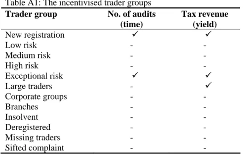
risk”. We focus in our analysis on only the VAT trader groups, as the non-VAT trader groups have very sparsely populated output patterns, often with no output recorded for several weeks or months. A list of the VAT trader groups is included in Appendix Table A1.
2.2 The bonus structure
To be eligible for any bonus, a team had to meet a baseline level of performance on all its targets. These baselines were the same for both teams and included measures like customer service, analysis accuracy and training. The bonus was paid if the team achieved an additional 5% above the predefined baseline on a subset of five of these targets (specified below). The team received the maximum bonus if it achieved all incentive targets in full. If a team met all the baselines and at least 2.5% of the additional incentive targets, half the bonus was awarded. Otherwise, no bonus was paid. This structure was designed to deal with the multi-tasking problem, to ensure that teams did not simply focus all their energy on the incentivised tasks.
Both of the incentivised teams had the same five incentive targets. Two of the targets were associated with achieving a specific number of visits to businesses. These were increasing the number of audits by 5% over baseline on trader groups known as “new registrations” and trader groups known as “exceptional risk”. The other three targets required increasing the amount of revenue collected by 5% over baseline on the trader groups labelled as “new registrations”, “exceptional risk” and “large traders” (see Appendix Table A1). It is clear from HMCE documents (HMCE 2002) that the choice of trader groups to incentivise was taken at a high level, jointly between HMCE and HM Treasury, who were funding the pilot scheme. They chose the trader groups where the amount of unpaid VAT was likely to be greatest, and therefore the yield recovered also likely to be the highest. The incentivised outcomes (discussed in more detail below) are measured with a high degree of precision. The trial teams
were combined with a blind control team. The staff in the control team did not know that they were monitored, so there was no scope for observational effects.
Each trial team was subject to a different reward scheme. In Team 1 the absolute value of the bonus varied according to the individual’s grade (job band), worth 3% of salary. In Team 2, the absolute value of the bonus paid was equal across all team members, including the team manager. The average value of the bonus for each team as a whole was the same at about 3% of salary. Table 1 shows the values of the average potential bonuses in each team; given the different structures and the overall equality, the only non-trivial difference is for the manager. Our conversations with HMCE officials suggested that managers saw these bonuses as a worthwhile amount for the extra effort to achieve the targets. HMCE also had in place a standard promotion and progression system, and this continued throughout the trial period. Thus the career concerns of managers as well as the immediate financial bonus gave them incentives to improve the performance of their team to hit the targets.
The scheme generated direct, explicit, financial incentives for all team members, including the team manager. As noted above, because of the team basis of the reward, these were likely to be rather weak unless reinforced by managerial or peer pressure. The inclusion of the manager in the team meant that s/he was likely to be particularly important in effecting any change in performance through the allocation of workers to tasks. There may also be differential effects across tasks. The impact of a worker’s effort on the two incentivised tasks is different. For the number of audits, effort directly maps onto the outcome. But for yield recovered, the outcome will also depend on the nature of each case. More effort increases the probability of finding undeclared taxes, thereby raising tax yield, but the effect is less certain ex-ante.
Finally, the rationale for implementing the incentive scheme at all lies in the nature of the production process. Whilst the manager has the authority to assign workers to particular trader groups, the job of audit is not simple. There is a degree of professional judgement involved, and enough idiosyncratic details between cases to give rise to a moral hazard problem and hence the potential for an incentive scheme to be useful. Furthermore, there is a good deal of managerial skill involved in assessing workers’ abilities and matching them to particular types of cases. This effort is hard to observe and cannot be contracted. The incentive scheme was introduced to more closely align the goals of the workers and managers with those of the organisation as a whole.
3. Data
The scheme ran from April 2002 through December 2002. We use data from the agency’s performance management system and personnel records for this period and the equivalent nine months in the previous year. As there is a very strong monthly pattern to the workflow in HMCE we chose to use the equivalent nine months rather than the immediately preceding nine months. No data is available after the end of the scheme. The data are very disaggregated: we have records for each worker, by week, for each trader group. From this, we examine a set of outcomes. These are the time allocated by each worker to each trader group, total yield per worker per trader group, and productivity (defined as yield relative to time, weighted by the share of time spent on the trader group). As we do not have a direct measure for the number of visits to businesses (this is the incentivised outcome), we use the time spent on each trader group as a proxy for this. The other incentivised outcome (revenue) is measured directly as yield. We aggregate the weekly data into monthly outcomes as many
of the worker*week*trader group observations are zero.
Table A2 describes the raw outcome data, distinguishing between the three teams and the two periods.4 It shows that, on average in the pre-incentivisation year, each worker worked on 2.9
different trader groups in a typical week, with little variation across the three teams. During the incentivised year, the average number of trader groups was higher (4.5), but remained similar across the teams. The average number of hours per trader group per week is somewhat higher in the pre-incentivised period (9.29 hours) compared to the incentivised period (7.91 hours), with team 1 spending slightly less time in both periods on VAT activities compared to team 2 and the control team. There is a great deal of variability in time allocated across workers, weeks and trader groups. The incentivised groups – new registrations and exceptional risk traders – account in the incentivised period for 31% and 25% respectively of total audit time allocated in team 1, 37% and 30% in team 2, and 37% and 28% in the control team.
After completing an audit, workers record the monetary value of the outcome. The mean yield collected on VAT trader groups in the pre-incentivised period is £6,953 per worker per week per trader group. However, this figure reflects the presence of some very large outlier values (to which we return below); the median yield per worker per week per trader group is, in fact, zero. Team 2 has a slightly higher average yield in both periods compared to team 1 and the control. The average yield obtained by the control team in the incentivised period is lower than both teams 1 and 2. The largest share of yield in the incentivised period comes from the “exceptional risk” trader group in all three teams, accounting for 44% of yield in team 1, 45%
4
Details of non VAT activity are available at
in team 2 and 47% in the control team. New registrations and high risk groups follow in order of magnitude.
As noted, the yield distribution has some very large outliers. In these administrative data, all yield obtained on a certain trader group will be allocated to a specific week, even if the worker has spent several months on that case. And as the data are at worker*week*trader group level, there are also many zero records. Modelling this is not straightforward: all yield observations count towards the teams’ targets and therefore are ‘legitimate’ observations. The zeros and the very high observations are not measurement error. Hence, the use of mean regression as a method of analysis is one legitimate approach. However, including the very large yields may risk distorting our estimate of typical underlying behaviour. We examined various different ways of taking this into account, including trimming the data to exclude large outliers, taking logs and estimating quantile regressions. In the results reported here, we deal with this issue in two ways. First, we report quantile regressions alongside the OLS for the key specifications. Second, we use tobit regressions to account for the large number of zero records in the distribution of yield. We do not analyse the log of yield for two reasons. First, zero yields do not transfer to logs. Second, and more importantly, our estimation strategy involves summing up (differenced) yields over workers or months. As we cannot sum up the logs, and as differenced yields may be negative, we report all results in levels.
In all analyses, we choose to omit one observation of a worker from team 2 who obtained a yield of £160 million in one week on the incentivised “exceptional risk” trader group. This is by far the largest yield observation in the data. Including this number would increase the mean yield collected on VAT trader groups for team 2 to £29,055 (standard error £1,735,666) for team 2 in the incentivised period. Our qualitative results are not affected by this large
number, although it increases the estimated coefficients for team 2 significantly.
We make two selection decisions for our worker-level analysis. First, we focus only on those staff who are employed throughout the observation period; this includes the managers. This removes only two workers from the dataset for each team, so it is clear that worker turnover and selection are not an issue in any response to the scheme. Second, we analyse frontline staff only. These are defined as workers who register time on audit and collect tax. The vast majority of frontline staff are workers in job bands 6 and 7, with a small number in the lower bands of 4 and 5 and the higher bands 8 and 9 (band 9 is an office manager grade). The number of these frontline workers who are continuously employed is 129 in team 1, 124 in team 2, and 197 in the control team. The remainder of the continuously employed staff are either clerical workers (10% across all teams and both time periods) and office or team managers (5%). There is one team manager (job band 11) per team.
Our main identification strategy is a difference-in-difference-in-difference approach. We exploit variation before and after the introduction of the scheme, between treated and control teams, and between incentivised and non-incentivised trader groups. The validity of this depends on the absence of other major factors causing a change in behaviour at the same time, and on comparability between treatment and control groups. Our discussions with the HMCE officials conducting the scheme indicated that there were no other major policy changes at the same time as the team based pay experiment. The organisation’s personnel and performance management systems and objectives were well established at this stage. Of course, in any large public organisation there are always minor “initiatives” that appear from the centre, but there were none in this case that might have had a material impact on outcomes.
To establish the comparability of the three teams, we provide descriptive statistics in Table 1. All three teams are similar in staff composition: average age and tenure, proportion female, days of sick-leave, fraction of part-time workers, over-time worked and annual pay are all very similar. Average pay is slightly lower in the control team, because of the slightly lower age and tenure. The two treatment teams are essentially the same size, although the control team is somewhat larger. The teams served similar areas, focussed around middle-sized cities. Team 1 were located in three offices and team 2 in six offices. We do not have information on the location of the offices, hence we cannot control for possible differences in geographical characteristics. Our data also do not tag workers to offices, so we cannot look for potential effects of office size. Team size is a well-known issue in understanding the impact of incentive schemes in teams (see Holmstrom, 1982). However, with just three observations at team level, this issue cannot be explored here.5
In addition to variation across time and team, the analysis also exploits a third level of variation, between incentivised and non-incentivised trader groups within teams and periods. As nothing in the production function changed across groups with the introduction of the scheme this seems a very strong source of variation.
4. Estimation results
This paper addresses two questions. First, what is the impact of the scheme on team-level outcomes and, second, how does this effect come about? The bulk of our results are focussed on the second question. Specifically, we examine whether any observed change arises chiefly through greater effort or through a reassignment of tasks to different workers by the team
5
Burgess et al., 2007, studies the introduction of team based incentives in employment offices in the UK and focuses on the effect of variation in size across those offices.
manager.6 To answer these questions, we first consider the impact of the scheme at team and
team*trader group level, and then evaluate the impact on individual performance and task allocation.
4.1 Team and team*trader group level analysis
We report two analyses at team level: the first does not distinguish by trader group, the second does. We adopt a simple linear additive model of production at team and monthly level:
gm g m gm gm
y =α +λ +βD +u (1) where ygm is the outcome variable (respectively visits (proxied by time spent), yield, and productivity); g indicates team (1-3) and m month (1-9). Dgm is a dummy for the incentive scheme operating in that team at that point in time and ugm is the error term. The treatment effect is β. This specification controls for team and month fixed effects. Team effects incorporate the nature of the local business environment, the human capital composition of the team, managerial ability and so on. The underlying time series dependence is likely to be complex, as during the incentive period, managers will monitor and react to the gap between the cumulated output and the target. However, modelling this complex non-linear dependence is beyond the scope of this paper. In modelling the error term, we allow for simple serial correlation with an AR(1) term and estimate separate treatment effects for team 1 and team 2.
Our three outcome variables are not all equivalent. Time and yield are both directly incentivised, but productivity is not. Logically, there is no reason why productivity on incentivised tasks has to increase. It may be easier to raise productivity on the other tasks, transfer the time saved to the incentivised tasks and hit the targets in that way; a negative response of productivity to the scheme is consistent with a rational response to the scheme.
6
Nevertheless, we are interested in the response of the productivity outcome (in addition to the two directly incentivised outcomes) as this is essentially the social interest in this scheme – whether the introduction of incentives for this group of public sector workers improves overall performance.
The results of this difference-in-difference analysis are presented in Table 2. Table 2 shows three team-level outcomes (time, yield, and productivity) and uses three specifications (OLS, AR(1) and quantile regression). The results are similar for the two treatment teams. The table shows a slight increase in average time at team level in both teams during the incentivised period. On average, team 1 increased its time in the incentivised period by 4.5 hours per worker per month compared to the control group. Team 2 increased its time by 5.93 hours per worker per month compared to the control. Allowing for an AR(1) error, only the effect in team 2 remains significant. The quantile regressions show significant increases for the bottom 25th percentile of time for both teams. Yield is larger for both treated teams during the
incentivisation period, but the estimates are not statistically significant. However, both treated teams have an positive incentivisation effect for productivity at the mean; this is also significant at the median in team 1.
The research design involves variation in incentivisation not only across time and treatment status, but also across trader groups. This provides us with additional identifying power in the analysis. Our second team-level analysis uses this to estimate the difference-in-difference-in-difference specification
gtm g t m gt tm mg gtm gtm
y =α + +δ λ +τ +γ +η +βD +u (2)
where t indicates trader group, with the other subscripts as in equation (1). This second specification includes team, month and trader group fixed effects and all pairwise
interactions.7 The trader group dummies encapsulate the specific difficulties and issues of
working with particular types of firms. For example, small firms will have different audit characteristics to very large firms; different ratios of time to yield are likely between complex cases where tax under-declaration is thought very likely to more standard cases where a more cursory audit may be appropriate. As throughout, treatment status is a group variable: there is variation in the change in treatment status only across three teams and across the trader groups, not at worker level.
We identify the effect of the scheme in (2) through the difference between incentivised and non-incentivised tasks. For the productivity outcome this is straightforwardly interpretable since there is no reason to expect productivity in the non-incentivised tasks to change. For time (and therefore yield), to the extent that there is a fixed overall budget of time to be allocated across the two tasks, the estimated difference incorporates both a possible rise in the incentivised tasks and a fall in the non-incentivised tasks. However, in our case, there is not a fixed overall budget as team managers are also able to switch staff time into these audit tasks at the expense of non-audit time. So our estimates with respect to the time outcomes lie between a pure net addition to time and a pure zero-sum reallocation.
The findings of equation (2) are presented in Table 3. In addition to the OLS, AR(1) and quantile regressions, we also report the results from a tobit specification for yield and productivity. Analysis at the trader group level (so distinguishing between the incentivised and non-incentivised trader groups) within teams shows a significant negative treatment effect
7
Clearly, the errors are not independent across g*t*m observations. We respond to the nature of the treatment by providing standard errors clustered at team level, but we are aware that this is not a complete response (see for example, Donald and Lang, 2007, who investigate the inference properties of difference-in-difference estimators with variables fixed within groups).
for time and productivity for team 1. All other specifications show no significant effects for team 1. For team 2, the results show much stronger effects from the scheme with significant increases in all outcomes of time, yield and productivity. In addition, the different model specifications present coefficients that are very similar in magnitude, though the quantile regression estimates are generally not significant. Team 2’s treatment effect for time in the OLS and AR(1) specifications is about 5 hours per trader group and month. Thus, on average, team 2 increased its time on incentivised trader groups by 5 hours per month per worker relative to the change in time spent on non-incentivised trader groups compared to that of the control team. The OLS, AR(1), and tobit regressions all report an increase in yield and productivity for team 2 relative to the control ranging from £11,380 – £12,050 per month per worker and £272 – £287 per month per worker respectively. Had we included team 2’s large outlier of £160 million in these analyses, the picture that Team 2 does more in response to the incentivisation does not change. However, we would obtain much larger estimates than those reported in Table 3: the range would be between £62,180 – £63,730 per month per worker for yield and £1,412 – £1,449 per month per worker for productivity. Time, of course, is not affected. These results are consistent with the outcome of the scheme in terms of the teams hitting their targets and being awarded the bonuses as team 2 hit its targets while team 1 did not.
Thus although Table 2 shows both teams increased their time in the incentivised period relative to the pre-incentivised period, Table 3 shows that only team 2 did so on the incentivised trader groups. In addition, the team-level analysis above (Table 2) shows no significant coefficients on yield and only slight effects on productivity. Once we allow for trader group differences however, the results show significant improvements in team 2’s performance, with no or negative effects for team 1.
4.2 Individual level analysis
The remaining part of this paper examines how the effects described above come about. More specifically, we explore whether the effects can be attributed to increased worker effort or to better assignment of workers to tasks by managers. This section considers the former; the role of task reallocation will be addressed in the next section.
Adopting the individual counterpart to the team level equation (2) above, we assume that individual output is determined by personal characteristics such as age and experience (X), in addition to the trader group, time and team factors as discussed above, and the treatment effect. For each worker and trader group, we sum up the outcome variable for the nine months of the incentivised period and the nine months in the year prior. We then take the difference, giving us the change in the outcome variable over the nine-month period for each worker and trader group:
9 9
, ,
1 1
itm incentivised itm pre incentivised it t it i it
m m
y y − y δ βD γ
= =
− = Δ = + +
∑
∑
X + , u (3)where we include two treatment effects; one for each team. Differencing removes the simple linear effects of the team and trader group dummies and the time-invariant worker characteristics, although we do still condition on these variables in the regression to allow for any differential impacts on the change. As the change in treatment status varies across the three teams and across trader groups (but not at worker level), we allow for correlation among the errors at team*trader group level.
The results are presented in Table 4. The reported coefficients are the treatment effects from a difference-in-difference-in-difference estimation at the worker*trader group level. The story
is slightly different to that in Table 3, which showed large and significant positive treatment effects for productivity only for team 2, with negative estimates for team 1. The worker level analysis in Table 4 now shows a slightly larger increase in productivity for team 1 compared to team 2. With less time spent on incentivised trader groups, but slightly more yield, the productivity per worker in team 1 actually increased, and by a larger amount than that of team 2. Thus we have a situation in which team level productivity increases significantly more in team 2, but individual productivity increases slightly more in team 1. Part of the clue as to what is happening is in the first column of the table. This shows that individual workers on average contributed a lot more hours per month to the incentivised trader groups after the scheme in team 2, relative to the control team, but also relative to the gap between team 1 and the control group.8
This difference in response at individual and team level suggests that the strategy at team level differed between the two treated teams. An important part of team strategy is the allocation of workers across trader groups. Managers can strategically allocate more efficient workers to incentivised trader groups in order to meet the targets. In what follows, we investigate how the allocation of efficient workers differs across the two treated teams and the control team.
4.3 Strategic task allocation
The richness of our data permits a detailed investigation of the allocation of individuals to different trader groups, and how this changes over time. We explore whether high productivity individuals in the first period were allocated to the incentivised trader groups in
8
In results not reported here, we investigated whether workers with different characteristics respond in different ways to the scheme. We matched workers in the treated teams with those in the control team by observable characteristics (job band, age, gender). The results showed no consistent and significant differences in terms of average outcome changes.
the incentivised period. We identify efficient workers as those in the top quartile of the productivity distribution in the period before the scheme. We analyse whether there is a significant difference in the reallocation of time on the incentivised and the non-incentivised trader groups by efficient workers and other workers per team.
Table 5 presents the average efficient workers’ and others’ time reallocation between incentivised and non-incentivised trader groups for each team, measured as the average change in hours per worker between the two nine-month periods. The table shows that both treatment teams increase total audit time by over 200 hours over the nine-month incentivised period compared to the same nine month in the year prior to the scheme.9 However, team 1
essentially splits this extra time evenly between the incentivised and non-incentivised trader groups. That is, it does little reallocation of its resources. The opposite is the case for team 2. It increases its time on incentivised trader groups and decreases its time on the non-incentivised tasks. Distinguishing between efficient and other workers, we see that both types increase the time spent on incentivised trader groups in both treatment teams. However, the largest increase is by efficient workers in team 2. It is clear that the time of efficient workers in team 2 is reallocated to incentivised trader groups much more than in the other two teams. Not only is all the increase in total audit time all allocated to the incentivised tasks (276 hours), but existing time is also strongly reallocated away from the non-incentivised tasks (the change is -122 hours). There is also a change in time allocation in the control team away from non-incentivised tasks. This is unexpected but given the random choice of the control group this is presumably an idiosyncratic outcome that would average out to zero if we had more control groups. It is clear, however, that the successful team, team 2, engaged in the
9
Overtime hours increased very little during the scheme in both teams, so that the increase in total audit time comes from other, non-audit, activities. It is not clear that this policy of reducing non-audit time would be sustainable over the long run; it may have been an explicitly short-run response to a short-run scheme.
reallocation of its most productive workers towards the incentivised trader groups to a far greater extent than the other treated team or the control team.
We use regression analysis to test the statistical significance of these patterns. We follow the same general set up as (2) above to analyse the reallocation. First, we examine how the time of efficient workers is allocated across trader groups by computing the fraction of all trader group time spent by efficient workers that is allocated to incentivised trader groups. Second, cutting the data the other way, we ask what fraction of the time allocated to incentivised trader groups is delivered by efficient workers. We would expect both of these fractions to increase in the period when the scheme operated in the treated teams. From what we have seen in Table 5, we would expect a bigger effect in team 2. These analyses are both at team*month level. For each of these variables in turn we estimate:
gm g m gm gm
y =α +λ +βD +u (4) where again g signifies team, m month, and β is the treatment effect. The results are in columns (1) through (4) of Table 6. The patterns are striking. Considering first the allocation of time of efficient workers on incentivised trader groups (column (1)), we find a large and highly significant treatment effect for team 2. Relative to the control team, in the second period, efficient workers spend 14 percentage points more of their total audit time on incentivised trader groups. In team 1, the treatment effect is in fact negative. Column (2) confirms these results in a quantile regression, which shows significant positive effects in team 2 and negative effects in team 1. The quantile regression shows a stronger positive treatment effect at the median and lower quartile than at the top of the distribution. This makes sense; it is likely to be harder to push a high fraction even higher without completely removing efficient workers from other tasks.
We find complementary results for the fraction of time allocated to incentivised trader groups that is delivered by efficient workers in columns (3) and (4). The OLS estimates show a significant positive treatment effect in team 2 and zero effect in team 1. The quantile regressions again confirm these findings. Team 2 increased the average productivity of workers working on incentivised trader groups by reallocating its best workers to these tasks, increasing the fraction of their labour input by an average 8 percentage points.
Finally, having looked at team-level, we now return to the underlying worker*trader group data to estimate the treatment effect. For each worker i, we compute nine monthly differences in time spent on all incentivised trader groups. Similarly, we compute the monthly differences for all non-incentivised trader groups. Including team, month, efficient worker and incentivisation dummies with its interactions, we estimate a treatment effect as the change in hours spent on incentivised trader groups, in the treated teams, by efficient workers:
, ,
icm incentivised icm pre incentivised
icm g m e c gc ce eg gce icm
y y
y α λ ν δ τ γ η βD u
−
− =
Δ = + + + + + + + + (5)
where c the indicates aggregated trader group (note that we distinguish only between whether the trader group is incentivised or not; we do not separate out all 12 trader groups), and e stands for efficient worker. Column (5) in Table 6 shows a significant positive effect for team 2 and one indistinguishable from zero for team 1, results which are consistent with columns (1) through (4) of the table. The results show that time spent by efficient workers in team 2 on incentivised relative to non-incentivised trader groups compared to other workers in their team rose by 18.9 hours per month compared to the control team.
As noted above, the incentive scheme took account of multi-tasking issues, as teams had to fulfil a set of base targets for all activities to be eligible for the bonus. This meant that teams
could not simply direct all effort at the incentivised tasks, but had to make sure that the other jobs were done. This made the optimal reallocation of worker time more subtle, and it appears
at team 2 made a better job of this.
n-difference design coupled with the stability of the workforce allows us to le this out.
th
We discuss possible reasons for team 2’s better performance in the Conclusion, but we can rule out a number of possibilities here10. It might be that workers in team 1 are more
homogeneous in productivity, leaving less scope for reallocation. In fact this is not the case: the pre-scheme dispersion of productivity is greater in team 1 than team 2. Secondly, it might be the case that all the best workers were already assigned to those particular trader groups. Again, the data do not bear this out – the efficient workers in Team 1 were split evenly between the incentivised and non-incentivised Trader Groups in the pre-scheme period as shown in Table 5. Kernel density estimates of the hours distribution by incentivisation status, team and period, (available from the authors), suggest that the hours distributions in the pre-period in both incentivised and non-incentivised groups were very similar in both teams. Staff composition might be such that workers in team 2 were on average more experienced than team 1 and hence better suited to reallocate their effort towards the incentivised trader groups. In fact, we show above there are only marginal differences in experience (see Table 1), and the difference-i
ru
4.4 Decomposition of the overall incentivisation effect
We now examine how much of the change in a team’s yield is due to the reallocation of workers and how much to greater effort. We denote the productivity of worker i in trader group j in period t as ψijt. It is measured as the ratio of total yield (Y) collected by that worker
10
in that trader group to the time spent (T) on that trader group by that worker. The increase in total yield at team level between the two periods can be decomposed as follows:
(
2 1)
1(
2 1)
2 1 2 ij j ij ij i ij j ij ij i T T T Y Y Y = − =∑
∑
− +∑
∑
− Δ ψ ψ ψ (6)ss team patterns in the change in total yield are ery similar when including all observations.
The first term represents the change in time allocated by worker i to group j. The second term captures the change in productivity for a given time allocation. We calculate this decomposition for our data and report the results in Table 7. Note that some workers spent time on incentivised trader groups only in one of the two periods, or collected yields in only one period. We lose these unbalanced observations, possibly affecting the randomness of the sample. However, we can only do this exercise for worker*trader groups with valid productivity measures in each period. Observations with positive yield but zero time are dropped.11 The number of workers with complete trader group records is 103 (team 1), 109
(team 2) and 119 (control).12 In the table, we report the change in total yield obtained from
these balanced observations. However, the acro v
The top line of table 7 shows the value of the change in yield. The second line shows the fraction of the change in yield on incentivised trader groups accounted for by the reallocation of time. This is 75.3% in team 1, 93.5% in team 2 and 85.2% in the control team. These results confirm our findings for the strategic reallocation of workers. In all teams, the change in yield of incentivised trader groups is explained mostly by an increase in the time spent on incentivised trader groups. This effect is particularly strong for team 2. Interestingly, if we look at the decomposition of the yield change for non-incentivised trader groups, we see that
11
We lose 6.7% observations in team 1 in period 1, 30.4% in the same team in period 2; 5.3% and 27.7% in team 2 in the first and second period respectively; and 11.2% and 31.6% in the control team.
12
We have tested the robustness of the other results to dropping the observations required for our approach. The results are robust to this reduced sample size.
reallocation in team 2 impacts there: the reallocation of the more productive workers away from the non-incentivised tasks by itself would have reduced yield there. By comparison, in team 1 and the control team, reallocation per se affects both outcomes positively, confirming
e less focussed reallocation in team 1 relative to team 2.
. Conclusion
nd collected the bonus. The other team eam 1) did not hit its targets and received no bonus.
ably representative of the level of onuses that would be paid in a large public organisation.
th
5
This paper has examined the impact of team based incentive pay in a large public sector organisation. The scheme was introduced as an experiment, allowing us to identify the impact of the scheme using difference-in-differences and difference-in-difference-indifferences. The robustness of this design allows us to examine the impact of the scheme and its effect on increased productivity versus task reallocation. We find that the incentive scheme raised individual productivity but also led to the reallocation of efficient workers towards the incentivised tasks. This reallocation was the more important contributor to the overall outcome. The increase in individual productivity was essentially the same in the two teams subject to the scheme, but the successful team (team 2) engaged in reallocation to a significantly greater degree than team 1, hit its targets a
(t
There are a couple of specific features of the incentive scheme that need to be borne in mind. First, the scheme only lasted nine months. Second, the bonus amounts involved were not large. However, they were not trivial and they are prob
b
have identified. First, the result could be due to a difference in the structure of work across the two incentivised teams, which existed prior to the introduction of the scheme. The successful team might have had a more flexible task assignment strategy because workers are used to dealing with different trader groups, so that they have enough experience to be effectively reallocated across trader groups. However, there is little difference in the number of trader groups that each team worked with in the prior period. Second, the extent of strategic task reallocation could be due to differences in the managers in the two incentivised teams. The bonus scheme in team 2 provides an equal bonus to all workers, so that relative to managers in team 1, managers in team 2 would receive a lower bonus if succesful. If managers were only motivated by financial incentives we would expect managers in team 1 to be more proactive in strategic behaviour. But we actually find the opposite suggesting more intrinsic incentives may be at work. On average, office managers are somewhat younger in team 2, have been in their job band for fewer years and they have less experience in the organisation. In addition, the overall team manager in team 2 is much younger than the other two teams and has less experience of the organisation13. One possible explanation for the different
performance of managers in the two teams is therefore that the team and office managers in am 2 may have had sharper implicit incentives from longer term career concerns.
te
There is a paucity of empirical research on the nature of team performance in response to incentives: our results provide evidence on the effect of such schemes on the balance between increased effort and task-reallocation. We consider that our results can be generalised beyond this one organisation. First, the production technology is common: a group of workers with multiple tasks, a manager with the capacity to allocate their time over these tasks, and some but imperfect information on their abilities in these tasks. Our results relate to the efficacy of
13
She has been in that role for only one year, compared to four years for the team 1 manager and eight years for the control team manager.
oles at least, financial incentives should not be ruled out as one way of achieving that goal.
different ways of increasing output in such organisations, emphasising the importance of task assignment with heterogeneous workers and key role of managerial discretion in that regard. Second, our results speak to the long-standing question of whether financial incentives are relevant or effective in the public sector at all. It is clear that some particular aspects of many jobs in the public sector are absent from this organisation; for example, this is not a “caring” role, and “mission” focus is unlikely to be strong. Nevertheless, a large number of jobs throughout the public sector are also not directly “caring” roles, and raising their productivity is an important policy issue. Our evidence suggests that for such r
Table 1: Team Descriptive Statistics
Total Job bands 6-7 Job bands 8-9 Job band 11, division manager Team 1 Team 2 Team 3 Team 1 Team 2 Team 3 Team 1 Team 2 Team 3 Team 1 Team 2 Team 3
Number of workers 129 124 197 110 113 151 6 3 5 1 1 1 Age 44.0 44.6 41.9 43.8 45.3 43.2 49.9 42.7 46.0 47 39 54 (9.1) (7.8) (9.6) (8.7) (7.4) (8.0) (4.7) (7.1) (7.6) Proportion Female 0.4 0.4 0.5 0.4 0.4 0.5 0.0 0.3 0.4 1 1 0 (0.5) (0.5) (0.5) (0.5) (0.5) (0.5) (0.0) (0.6) (0.6) Years in organisation 18.3 19.1 17.3 18.9 19.8 19.2 24.7 20.3 26.4 26 20 34 (8.7) (8.5) (9.7) (8.3) (8.4) (8.8) (7.4) (6.7) (7.2)
Years in job band 10.0 11.9 9.2 10.6 12.6 10.3 5.6 4.7 2.6 4 1 8 (8.2) (7.3) (8.1) (8.4) (7.2) (8.0) (4.9) (6.4) (3.3)
Days of sickness 1.2 1.0 1.4 1.2 0.9 1.5 0.4 0.0 0.0 0 0 0
(4.4) (4.0) (4.7) (4.4) (4.0) (4.5) (1.1) (0.0) (0.0)
Proportion Part-time 0.2 0.1 0.2 0.2 0.1 0.2 0.0 0.3 0.2 0 0 0
(0.4) (0.3) (0.4) (0.4) (0.3) (0.4) (0.0) (0.6) (0.4)
Hrs overtime per month 0.1 0 0 0.1 0 0 0 0 0 0 0 0
(0.3) (0.0) (0.0) (0.3) (0.0) (0.0) (0.0) (0.0) (0.0)
Potential bonus (£) 688 681 - 701 696 - 979 735 - 1520 740 -
(213) (135) - (152) (112) - (283) (11) -
Annual pay (£) 20020 20175 18750 20193 20494 19966 28035 26796 28638 37112 36140 38154 (3605) (3066) (4029) (2480) (2249) (2426) (2905) (4333) (2481)
Table 2: Team Level Impact of the Scheme; Difference-in-Difference
Time (in hours per month) Yield (in £ 1,000’s) Productivity (in £ 100’s per hour)
[1] OLS [2] AR(1) [3] Quantile [4] OLS [5] AR(1) [6] Quantile [7] OLS [8] AR(1) [9] Quantile Treatment effect Team 1 4.50* 3.21 31.29 32.74 186.69** 188.66*
(2.23) (3.28) (20.99) (42.30) (79.29) (95.62) Q25 7.00* 27.82 79.91 (4.05) (48.74) (88.64) Median 2.57 30.76 167.84* (3.23) (28.15) (89.31) Q75 2.90 32.09 130.94 (4.45) (38.38) (78.81)
Treatment effect Team 2 5.93** 8.20** 40.65 38.12 157.42* 158.18 (2.22) (3.28) (26.08) (42.30) (81.82) (95.62) Q25 8.27*** 15.96 19.51 (3.04) (53.46) (95.05) Median 4.10 33.20 85.32 (2.73) (45.05) (67.89) Q75 3.19 63.84 106.11 (4.08) (51.80) (78.21) Rho 0.424 -0.320 -0.129 Observations 54 51 54 54 51 54 54 51 54
Notes: The unit is team*month, and the analysis is carried out per worker. Other controls are team fixed effects and a full set of month dummies. Robust standard errors in parentheses. The standard errors on the quantile regressions are bootstrapped using 20 replications. * Significant at 10%, ** significant at 5%, *** significant at 1%
Table 3: Team*Trader Group Level Impact of the Scheme; Difference-in-Difference- in-Difference
Time (in hours) Yield (in £ 1,000’s) Productivity (in £ 100’s per hour)
[1] OLS [2] AR(1) [3] Quantile [4] OLS [5] AR(1) [6] Quantile [7] Tobit [8] OLS [9] AR(1) [10] Quantile [11] Tobit
Treatment effect Team 1 -0.83*** 1.07 0.69 0.33 0.49 -0.25* -0.46 -0.29 (0.01) (2.00) (0.31) (6.22) (5.41) (0.07) (1.55) (1.340) Q25 0.68 -0.36 -0.07 (2.34) (4.13) (0.93) Q50 1.02 0.94 0.97 (2.68) (3.71) (0.97) Q75 -0.95 2.72 0.73 (4.60) (3.66) (1.72)
Treatment effect Team 2 5.31*** 5.31*** 11.38*** 12.05** 11.38** 2.72*** 2.87** 2.72** (0.02) (1.27) (0.52) (5.58) (5.36) (0.13) (1.40) (1.33) Q25 7.21*** 1.85 0.18 (2.74) (3.38) (0.84) Q50 0.66 4.70 0.38 (5.87) (3.69) (0.90) Q75 3.47 5.38 0.12 (4.03) (4.09) (1.18) Rho 0.597 -0.144 -0.134 N 547 535 547 547 535 547 547 547 535 547 547 Notes: The unit is team*trader group*month, and the analysis is carried out per worker. Only VAT trader groups are included in the analyses. Other controls are a full set of team, month and trader group fixed effects, and all its interactions. Standard errors are clustered by team and reported in parentheses. The standard errors on the quantile regressions are bootstrapped using 20 replications. * Significant at 10%, ** significant at 5%, *** significant at 1%
Table 4: Impact on Individual Worker Outcomes; Difference-in-Difference-in-Difference
Time (in hours per month)
Yield (in £ 1,000’s)
Productivity (in £ 100’s per hour)
Treatment Effect Team 1 -4.98** 41.60 2.05*
(7.61) (34.17) (1.15)
Treatment Effect Team 2 38.66*** 155.34*** 1.95**
(13.55) (53.35) (0.94)
No. of Observations 2,296 2,296 2,296
Notes: The unit is the change in outcome for a worker in a trader group. OLS regression, also controlling for team membership, years in job band, age, mean age squared, gender, part-time/full-time worker, job band, all trader groups. Only VAT trader groups are included in the analyses. Robust standard errors are given in parentheses and are clustered by (team*trader group). * significant at 10%, ** significant at 5%, *** significant at 1%
Table 5: Strategic task reallocation (time, in hours)
Team 1 Team 2 Control
Change in total audit time 205.5 244.2 33.8
Incentivised Trader Groups
Pre- and post-incentivisation Pre Post Pre Post Pre Post
Audit time, Efficient workers 260.4 347.5 246.1 522.0 326.0 374.5
Audit time, Others 196.8 231.8 267.6 366.4 199.5 245.4
Change in audit time (post-pre)
Efficient workers 87.1 275.9 48.5
(29.4) (45.4) (42.4)
Others 35.0 98.8 45.9
(16.4) (24.6) (16.4)
Significance of t-test * ***
Non-Incentivised Trader Groups
Pre- and post-incentivisation Pre Post Pre Post Pre Post
Audit time, Efficient workers 232.5 261.8 317.5 195.3 276.2 186.9
Audit time, Others 147.1 201.2 239.1 230.8 155.5 184.2
Change in audit time (post-pre)
Efficient workers 29.3 -122.2 -89.3
(29.9) (37.7) (29.9)
Others 54.1 -8.3 28.7
(15.5) (20.7) (13.1)
Significance of t-test *** ***
Notes: The table shows the average change in time spent per worker between the two nine-month periods on incentivised and non-incentivised trader groups. Standard errors are in parentheses. T-tests are of the equality of means between efficient workers and others. * significant at 10%, ** significant at 5%, *** significant at 1%
Table 6: Analysis of Task Reallocation
Dependent variable: # hours spent on incentivised trader groups by efficient officers # hours spent on all trader groups by efficient officers
# hours spent on incentivised trader groups by efficient officers
# hours spent on incentivised trader groups by all officers Δtimeicm
[1] OLS [2] Quantile [3] OLS [4] Quantile [5] OLS
Treatment effect Team 1 -0.09** 0.03 -4.86
(0.04) (0.02) (8.22) Q25 -0.09 0.02 (0.06) (0.03) Q50 -0.09* 0.03 (0.05) (0.03) Q75 -0.09 0.01 (0.06) (0.03)
Treatment effect Team 2 0.14*** 0.08*** 18.93*
(0.04) (0.02) (10.85) Q25 0.14** 0.07*** (0.07) (0.03) Q50 0.15** 0.08*** (0.06) (0.02) Q75 0.10 0.10*** (0.07) (0.03) N 54 54 54 54 8,100
Notes: Only VAT trader groups are included in the analyses. Team and month dummies are included as covariates in all regressions. In [1] through [4] the unit is a team*month. In [5] the unit is a worker (i)*monthly change (m)*aggregated trader group (c). The dependent variable in column [5] is the worker level monthly change in time spent on incentivised and non-incentivised trader groups. The treatment effect is the interaction between the efficient worker dummy, team dummies and a dummy for whether the trader group is incentivised. Efficient workers are defined as those in the top quartile of the productivity distribution in the pre-incentive period. Robust standard errors in parentheses. * significant at 10%, ** significant at 5%, *** significant at 1%
Table 7: Decomposition of the change in yield
Team 1 Team 2 Control Team
Incentivised Trader Groups
Value of Change in yield (£m) 13.945 21.164 5.083
Due to time reallocation (%): 75.3 93.5 85.2
Non-incentivised Trader Groups
Value of Change in yield (£m) 8.026 11.214 -2.376
Due to time reallocation (%): 5.1 -18.8 41.9
Number of workers 103 109 123
Notes: Only VAT trader groups are included in the analyses. We compute the decomposition as follows. We first assume that each worker*trader group productivity is the same in the incentive period as in the initial period, and multiplying this constant productivity by the change in hours spent by that worker in that trader group between the two periods. This change is added up over all workers in a team, and over the two types of trader groups shown in the table. This provides the fraction accounted for by time reallocation. The reverse procedure provides the fraction due to productivity change.
References
Baker, G., Gibbs and Holmström, B. (1994a) ‘The internal economics of a firm: Evidence from personnel data’ Quarterly Journal of Economics, 109, pp.881-921
Baker, G., Gibbs and Holmström, B. (1994b) ‘The wage policy of a firm’, Quarterly Journal of Economics, 109, pp.921-57
Bandiera, O., Barankay, I., and Rasul, I. (2007) ‘Incentives for managers and inequality among workers: Evidence from a firm-level experiment’ Quarterly Journal of Economics. vol. 122 pp. 729 – 773
Bandiera, O., Barankay, I., and Rasul, I. (2008) ‘Social Connections and Incentives in the Workplace: Evidence from Personnel Data’ forthcoming Econometrica
Burgess, S., and M. L. Ratto (2003) ‘The role of incentives in the public sector: issues and evidence’ Oxford Review of Economic Policy vol. 19 no. 2.
Burgess, S., Propper, C., Ratto, M. and Tominey, E. (2007) ‘Incentives in the public sector: Evidence from a government agency’. CMPO Discussion Paper, CMPO, Bristol. Dixit, A. (2002) ‘Incentives and organisations in the public sector: an interpretative review’
Journal of Human Resources, vol. 37 no. 4, pp.696-727.
Donald, S.G., and Lang, K. (2007) ‘Inference with difference-in-differences and other panel data’ Review of Economics and Statistics Vol. 89, No. 2: 221-233.
Encinosa, W., Gaynor, M. and Rebitzer, J. (1997) ‘The sociology of groups and the economics of incentives: Theory and evidence on compensation’ NBER Working Paper 5953, NBER, Cambridge.
Gaynor, M. and Pauly, E. (1990) ‘Compensation and productive efficiency in partnerships: Evidence from medical group practice’ Journal of Political Economy, vol. 98, pp. 544-74
Hamilton, B. H., Nickerson, J. A., and Owan, I. (2003) ‘Team incentives and worker heterogeneity: An empirical analysis of the impact of teams on productivity and participation’ Journal of Political Economy. Vol. 111 no. 3 pp. 465 – 497.
HMCE (2002) ‘”Incentives for Change” Team Bonus Trials Year 2, Q&A Briefing for Managers’. HMCE, London.
HMSO (1999) ‘Modernising Government’ www.archive.official-documents.co.uk
Holmström, B. (1982) ‘Moral hazard in teams’, Bell Journal of Economics, vol. 13, pp. 324-340.
Kandel, E. and Lazear, E. (1992) ‘Peer pressure and partnerships’ Journal of Political Economy, vol. 100, pp.801-817.
Knez, M. and Simester, D. (2001) ‘Firm-wide incentives and mutual monitoring at Continental Airlines’ Journal of Labor Economics vol. 19 pp. 743 – 772.
Lazear, E. (2000) ‘Performance pay and productivity’ American Economic Review, vol 90 no. 5, pp. 1346-1361.
Makinson, J. (2000) ‘Incentives for change. Rewarding performance in national government networks’ , Public Service Productivity Panel. HMSO, London.
Prendergast, C. (1999) ‘The provision of incentives in firms’ Journal of Economic Literature, vol 37, pp. 7 – 63.
Appendix
Table A1: The incentivised trader groups
Trader group No. of audits
(time) Tax revenue (yield) New registration 9 9 Low risk - - Medium risk - - High risk - - Exceptional risk 9 9 Large traders - 9 Corporate groups - - Branches - - Insolvent - - Deregistered - - Missing traders - - Sifted complaint - -
Table A2: Output statistics per worker, week, and trader group
Pre-incentivised period Incentivised period
All teams Team 1 Team 2 Control All teams Team 1 Team 2 Control Number of trader groups per worker, week
Mean 2.9 2.7 2.9 2.9 4.5 4.6 4.5 4.5
Standard deviation 1.26 1.25 1.24 1.27 1.42 1.47 1.45 1.35
Median 3.0 3.0 3.0 3.0 4.0 4.0 4.0 4.0
Time per worker, week, trader group (in hours)
Mean 9.29 8.96 9.25 9.54 7.91 7.11 8.50 8.04
Standard deviation 8.03 7.43 8.10 8.35 7.49 6.59 8.18 7.49
Median 7.5 7.5 7.3 7.5 6.0 5.8 6.4 6.0
% new registrations 42% 43% 42% 41% 35% 31% 37% 37%
% exceptional risk 15% 15% 10% 18% 28% 25% 30% 28%
Yield per worker, week, trader group (in £)
Mean 6,953 6,415 8,259 6,172 7,291 7,766 10,785 3,884 Standard deviation 195,426 85,537 252,885 191,190 153,198 102,214 247,538 34,112 Median 0 0 0 0 0 0 0 0 % new registrations 28% 44% 27% 19% 25% 27% 23% 23% % exceptional risk 21% 33% 12% 24% 45% 44% 45% 47% % large traders 3% 2% 6% 0.1% 4% 1% 7% 3% Observations 19,716 5,237 6,769 7,710 27,240 8,191 8,840 10,209