Impact of Trade Reforms in Tunisia on the Elasticity of Labor Demand

1

Impact of trade reforms in Tunisia on the elasticity of labor demand

November 2010

Abstract

The impact of trade reforms on the labor market may transit through many channels. One of these is the effect on labor demand elasticity emphasized by Rodrik (1997). No consensus has been established yet in the empirical literature regarding this relationship. This paper attempts to extend the work of Hasan et al. (2003) by disaggregating labor into skilled and unskilled categories in order to analyze the effects of trade policies on labor demand elasticities by skill in Tunisia. We use dynamic panel techniques to estimate a model of employment determination which incorporates the effects of trade and takes into account the delay of labor adjustment. Our database covers 529 Tunisian firms from 6 manufacturing sectors over the period 1997-2002. Results suggest that a decrease in trade protection in Tunisia increases the elasticity of unskilled labor demand while it contributes to reduce the elasticity of skilled labor demand.

Keywords: Trade liberalization; Trade and labor market interactions; skills; labor demand

elasticities, Tunisia

2

1. Introduction

The 1990s have witnessed a great deal of research emphasizing the rise of wage differentials between skilled and unskilled workers. This constitutes an important issue since growing inequalities contributes to weaken the social cohesion by its effects on poverty, especially if unskilled workers are not enjoying improvements in their situation in relative and sometimes absolute levels. What emerges from theoretical and empirical studies is that these changes in wage structure are linked in several developed and developing countries to trade liberalization reforms via their effects on skilled and unskilled labor demand. For a long time however, the driving forces behind labor demand movements have been put forward in the light of the Heckcher-Ohlin model and the skill-biased technological change. Yet, recently, a new issue of the trade-labor linkage has been highlighted in the context of imperfectly competitive market: trade liberalization might increase the own-price elasticity of labor demand, i.e. it makes the demand for labor more responsive to changes in its costs.

This new path was first emphasized by Rodrik (1997) who points out two main channels through which greater openness leads to an increase in labor demand elasticity. First, the substitution effect explains the employment variation due to substitution toward other inputs for constant output. Accordingly, trade liberalization leads to a release of input and equipment constraints that allows firms to use more imported capital and other intermediate inputs at lower prices. To the extent that these imports are substitutes for the services of domestic labor, substitution possibilities might increase.

Second, the scale effect depicts the employment variation due to the wage-induced change in the demanded output. The increased competition in the output market implies a rise in product market elasticity. This, in turn, increases labor demand elasticity given the Hicks ‘fundamental law of factor demand’ which states that ‘‘the demand for anything is likely to be more elastic, the more elastic is the demand for any further thing which it contributes to produce’’.

What are the implications of more elastic labor demand? Rodrik (1997) and Slaughter (2001) emphasize three important consequences. Rising elasticities imply more volatile reactions of employment to any exogenous shock to labor demand. They also shift the wage and/or employment incidence of non-wage labor costs towards labor and away from

3

employers. Furthermore, greater elasticities imply a decline in labor bargaining power and thus, amplify income inequality. Openness is likely to put labor markets under greater pressure, a situation which is socially undesirable.

No consensus has been established yet in the empirical literature regarding the relationship between trade reform and labor demand elasticity. In many countries, including much of the developed, these effects have yet to materialise. For instance, Slaughter (2001) that focuses on the U.S and Bruno et al. (2004) using a panel of developed countries present mixed evidences of the theoretically positive link between trade and labor demand elasticity. Krishna et al. (2001) and Fajnzylber and Maloney (2005) do not find empirical support in Turkey and Latin America respectively while Hasan et al. (2003) come upon a positive impact of trade liberalization on labor-demand elasticities in the Indian manufacturing sector. Our contribution to this debate is essentially an empirical issue.

Our paper investigates the impact of trade liberalization process in Tunisia on labor-demand elasticity by distinguishing different skills. The Tunisian economy should be an instructive case of study for at least two reasons. The first is that it would be complementary to current literature, widely focused on Latin American and Asian countries. It could improve the understanding of trade liberalization effects on labor demand elasticities in developing countries taking into account their specific economic liberalization processes. Second, Tunisia has been subject to an increase, however relatively moderate, in wage inequality subsequently to trade reforms introduced in 19861

We use micro level data covering 529 firms from 6 manufacturing sectors over the period 1997-2002. The attempt is to extend the work of Hasan et al. (2003) by disaggregating labor into skilled and unskilled categories in order to analyse the effects of trade policies on labor demand elasticities by skill. In fact, one could suspect that the absence of a statistically significant connection between these variables is due to the aggregation of employment that . Furthermore, Ghazali (2009) emphasizes the existence of a positive and statistically significant relationship between trade openness and wage inequality between skilled and unskilled workers. Greater labor demand elasticities might be an indirect channel through which trade effects on wage differentials transits.

1

Ghazali (2009) demonstrates that the 1970s and the first half of the 1980s were characterised by a reduction in wage inequality in the Tunisian non-agricultural productive sector. A skilled worker was paid in 1975 almost four times the wage of an unskilled worker. In 1985, the relative wages ratio is about 3. This ratio increased after 1986 attaining 3.42 in 1991. During the following years, wage inequality displays a slight decrease as the relative wage of skilled workers falls to 3.27 in 1998.

4

may hide compositional changes. Our empirical strategy consists in regressing a model of employment determination which incorporates the effects of trade on labor-demand elasticities. We take into account the delay of adjustment of labor as we suppose the existence of labor market adjustment costs that prevent a simultaneous regulation of firms’ employment to external shocks. We rely in the estimation of this dynamic model on the System Generalized Method of Moments (GMM) estimator as suggested by Blundell and Bond (1998).

This paper is organised as follows: section 2describes the Tunisian trade liberalization process.Section 3 focuses on the link between trade liberalization and firm’s own price labor-demand elasticity. Section 4 and 5lay down the framework of the empirical analysis as well as the database used. Section 6 presents the main econometric results. Section 7 concludes.

2. The Tunisian Trade Liberalization Process

Tunisia initiated a structural adjustment plan in 1986 that signed the start of the trade liberalization process. It entailed a process of lowering and setting uniform tariffs such that the average import duties declined from 41% in 1986 to 33% in 1987 and to 29% in 19902

2 _{Les Cahiers de L’Institut d’Economie quantitative (IEQ), n°9, Décembre 1991, p 51.}

. The highest duty rate was reduced from 200% to 43% (Bechri and Lahouel, 1999). The effective rate of protection (ERP) relative to all outputs excluding Hydrocarbon fell from 70% in 1986 to 44% in 1990. Trade reform pattern was not uniform across manufacturing industries over the period 1986-1991. For instance, unskilled intensive sectors as the food-processing and textile industries that benefited from a relatively higher protection level prior to trade liberalization observed a decrease of their effective protection rates by about 300 and 150 percentage points respectively. However, skill intensive sectors underwent either an increase of their rate of protection or a minor decrease within the same period. The ERP shifted from 40% to 82% in construction materials, glass and ceramics industry and from 88% to 101% in the electrical and mechanical industries. Concerning the chemical industries, the ERP moved from 88% to 78% between 1986 and 1991. Overall, skill intensive industries were less protected prior to the reforms. Therefore, they were subject to smaller reductions in tariff protection. Similar patterns of protection are reported in Colombia (Attanasio et al, 2004), Mexico (Hanson and Harrison, 1999) and Morocco (Currie and Harrison, 1997). In 1990, Tunisia signed the GATT agreements. The adherence to the WTO was achieved in

5

1995. Reflecting the government’s objective to comply with the GATT/WTO negotiated rates, Tunisia witnessed over the period 1990-1998 an increase in the nominal protection rates on agricultural final goods because of non-tariff protection transformation. The nominal protection rates on industrial final goods increased for the same reason while the nominal protection rates on industrial intermediate goods decreased due to the focus of the openness process at this stage on equipments and inputs. This led to an increase of the effective rate of protection for a majority of products (the ERP attained 56% in 1995 and 71% in 1998). The trade liberalization process has become more active since 1997 given that the effective rate of protection decreased from 71% to 49% in 2002.

3. Theoretical and empirical Background

Hamermesh (1993) considers the case of a representative firm which faces a perfectly competitive product market, constant returns to scale and variable inputs. He derives a firm’s demand for labor from a profit-maximising model of firm behaviour and he summarizes what determines a firm’s equilibrium own price labor-demand elasticity3 as following:

ε

σ

_L L Lw

s

s

E

=

−

(

1

−

)

−

4 Where L

s is labor’s share in firm total revenue, σ is the constant output elasticity of

substitution between labor and other factors of production and

ε

is the product-demand elasticity faced by the firm. All these variables are defined to be positive.

Equation (1) has two components. The first,−(1−s_L)

σ

represents the substitution term which indicates for a given level of output, how much the firm substitutes away from labor towards other factors when wages rise. International trade may affect labor-demand elasticity through its effect on the constant-output elasticity of substitutionσ . It expands the range of substitutes to new domestic and foreign factors of production acting either directly in foreign multinationals affiliates or indirectly through intermediate inputs, (Slaughter, 2001).

3 _{This elasticity is defined to be negative.}

4 _{This model assumes that the firm output is endogenous. If we assume a constrained (constant) output the}

elasticity will be

E

Lw

=

−

(

1

−

s

L

)

σ

and will represent purely the substitution effect. (See Hasan and al. (2003) for more details)

6

Differentiating (1) with respect toσ shows that as the firm substitution possibility set increases, labor demand becomes more elastic (i.e. E_Lwrises in absolute value).

(

1 _L

)

0 LW _S E − − = ∂ ∂ σ

The second part of equation (1), −s_L

ε

corresponds to the scale term. It points out how much labor demand changes after a wage change due to shifts in firm’s output. The increased availability of substitutes for the final good due to trade openness will make the output demand more elastic and reduces the scale of production consequently to higher costs.

Differentiating (1) with respect to

ε

shows that an increase in product-demand elasticity yields to a more elastic labor demand (i.e. E_Lwrises in absolute value).

0  L LW _S E − = ∂ ∂ ε

The greater is labor’s share in the firm’s costsS , the stronger is the pass-through from _L

ε

toE_{Lw (Slaughter, 2001).}

Accordingly, when wages rise, both the substitution and scale effects reduce labor demand. The industry substitutes away from labor towards other factors and with higher costs the industry produces less output such that it demands less of all factors.

The share of labor in total output may also decrease in response to trade openness which can make the direction of movement of labor-demand elasticity ambiguous. This makes empirical investigation in this area all the more important (Hasan and al., 2003).

The theoretically positive link between trade and labor demand elasticity remains elusive in empirical studies. A disagreement persists among analysts on the nature of recent trade reforms impacts on labor-demand elasticity. Exploring this link using data from the Turkish manufacturing sector, Krishna et al. (2001) do not find empirical support for the supposed theoretical relationship. Fajnzylber and Maloney (2005) use dynamic panel techniques to test the hypothesis that trade liberalization yields to higher own-wage elasticities of labor demand for manufacturing establishments in Chile, Colombia, and Mexico. The results do not provide evidence of a direct impact of trade liberalization on own-wage elasticities. Investigating the Indian case using data disaggregated by state and industry, Hasan et al. (2005) find a positive impact of trade liberalization on labor-demand elasticities in the Indian manufacturing sector. For the United States, however, Slaughter (2001) finds

7

mixed results. Proceeding in two stages, he first estimates a time series of own-price demand elasticities for production labor and nonproduction labor for manufacturing overall and for manufacturing disaggregated into eight industries. Second, he regresses the estimated elasticities on measures of trade, technology and institutional factors. The author finds that the U.S. production labor becomes more elastic in manufacturing overall and in five of eight industries within manufacturing from 1961 through 1991. Nevertheless, the elasticity of non production-labor demand does not exhibit the same trend during that period. Finally, the second stage results concerning the impact of trade on labor demand elasticities do not seem to be statistically robust to the inclusion of time controls.

4. The Model

This section outlines our specification of the model of employment determination which incorporates the effects of trade on labor-demand elasticities taking into account the delay of labor adjustment.

We start by assuming that a firm-specific production function can be described by a Cobb-Douglas form as following:

β α

γt t it it it D K L

y =exp(

∑

)

Where y indicates the output, K and L are capital and labor inputs, respectively. Capital stock is supposed to be fixed. α and β are parameters to be estimated representing factors shares coefficients. Dt is a dummy variable having a value of one for the tth time period and

zero otherwise and γ are parameters to be estimated. The year effects are introduced to take _t into account common aggregate shocks, particularly technological shocks that are not otherwise captured by our specification. Note that it is crucial to consider unobserved year-specific variables that could influence labor demand and labor demand elasticity (such as labor market regulation) concurrently with tariffs. The omission of year effects may bias the relation between tariffs and labor demand elasticity.

A firm’s demand for labor is derived from a profit-maximising model of firm behaviour and would therefore depend on output, stock of capital and the wage rate (w ), together with

the time dummies. However, the assumption of homogeneous workers in a firm can be

8

considered as a strong hypothesis since it is likely that firms employ workers of different skills. In particular, firms most often employ both skilled and unskilled workers. As long as data regarding different categories of workers are available, one can estimate disaggregated labor demand models (Bresson et al., 1992). This will permit us to analyse the effect of trade variables on labor demand and on labor-demand elasticities for different categories of skills. Consider that the firms’ production technology can be written as following:

)

,

,

,

(

_{it it}1 _it2 _t it

f

K

L

L

A

y

=

1 it

L is the level of employment of skilled workers, L_it2 is the level of employment of unskilled workers.

In the first stage we assume that firms determine an expected production and then minimize costs under the constraint of their expected level of production. Then the expression of the desired levels of employment for category j,L_it*jj=1,2 in terms of their determinants (capital, production level….), can be derived from the solution of the firm optimisation program. In our case they depend on the production level, on the capital stock K, on the wages w_it1 and w for the two worker’s categories considered together with the trade _it2

variables and the time trend (or dummies) which account for technical progress and common aggregate shocks. To control for product demand shocks and their effects on labor demand function we choose the conditional labor demand function (conditional on output).

The labor demand function for the category j can be written as:

)

,

,

,

,

,

(

_{it it} j k _{t i} j it

g

y

K

w

w

D

L

=

α

However, one should note that when firms face a change in their environment, particularly trade reforms, they do not necessarily immediately adjust their level of employment to the new business conditions due to the existence of adjustment costs, namely hiring and firing costs. To take this phenomenon into account, we use a dynamic adjustment process which can be represented as:

)

(

* ₁ 1 j it j it j j it j it

L

L

L

L

−

₋

=

λ

−

₋ (3) (5) (4)

9

Where

*

j it

L _{is the desired level (the optimum level) of employment for category j and} λ is j the adjustment parameter of the same category; L is the observed level of employment for _itj

category j. This would allow us to examine whether a firm’s response to trade shocks is related to the speed with which it adjusts to changes in desired employment levels. We suppose that the speed of adjustment depends on the skill level j. The dynamics of adjustment among labor inputs vary. One would expect that the higher the skill of workers, the higher the hiring costs, since training costs are expected to be lower for unskilled labor. Furthermore, since severance pay depends on the worker’s earnings and these depend on his skill, firing costs will increase with the worker’s skill (Borrego, 1998).

For analytical convenience and computational easiness, adjustment costs are assumed to be symmetric and quadratic to derive explicit partial adjustment models of labor demand (Bresson and al., 1992).

Thus, the labor demand function for category j can be rewritten as a reduced form equation for estimation: j it j i t j j it j j it i j j j i k j j i j j j it j j it j j j it j j it v D tpe tpe w w w K y L L + + + + + + + + + − = ₋

α

θ

λ

θ

λ

θ

λ

θ

λ

θ

λ

θ

λ

θ

λ

λ

4 6 5 4 3 2 1 1 ) ln( ) ln( ) ln( ln ln ln ) 1 ( ln

Coefficients are specific to the labor category j.

α

_{i is the firm’s specific effects. v}it captures

the idiosyncratic shocks. We assume that vit are not serially correlated.

As our main objective is to investigate trade liberalization effects on labor demand elasticities in Tunisia by skill category, we introduce interactive terms between wages and the effective rate of protection (ERP). This measure presents at least two advantages as emphasized by Goldberg and Pavcnik (2004) in their discussion on tariffs. The first is that ERP changes during trade liberalization reform episodes are not sector-uniform. They enable us to distinguish the effects of trade reforms from those of other economic reforms. The second advantage is that ERP movements in Tunisia, as in many other developing countries such as Brazil and Columbia, result from a governmental decision to fulfil the GATT and WTO directives. This would have the effect of minimising the endogeneity risk. The interactive term captures several effects exerted by trade openness such as broadening the set

10

of firm’s production techniques and inputs and increasing the productivity of existing inputs by new foreign knowledge and useful information, (Yasmin and Khan, 2005).

We also choose to include our trade protection indicator without interaction with other variables of interest in order to the direct effect of openness as labor demand shifter.

Highlighting the difficulty to conceive a perfectly satisfactory openness measure, Edwards (1998) suggests different proxies as robustness checks5. Thus, in order to measure trade liberalization, we have attempted to rely on another indicator which is the ratio of custom duties to imports CD/M that is seen as a good proxy variable for trade protectionism (Edwards, 1992). The rationale for both interacted trade terms (with ERP and CD/M respectively) is that a decrease in trade protection (that is an increase in the openness of the economy) raises labor demand elasticities. Thus, we expect a negative sign for the related coefficients.

5. The database

Our current firm-level database is the only firm-level data available in Tunisia. It was drawn from the national annual survey report on firms (NASRF) carried out by the Tunisian National Institute of statistics (TNIS) over the period 1997-2002. After the elimination of extreme outliers and observations that could be seen as erroneous, we have obtained an unbalanced panel consisting of a sample of 529 firms from 6 manufacturing sectors6

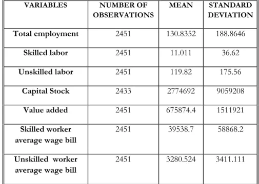
As shown in Table 1, the data include a large set of variables about value added (VA), number of workers (L) adjusted according to whether it is part or fulltime equivalent employment, capital stock (K), sales, expenditures disaggregated by equipment type, tangible and intangible fixed assets and firm indicators such as industry classification and the structure of equity participation (public, private, semi-public, foreign). We have also information about . We consider the period 1997-2002 as an interesting episode to capture the effects of trade reforms. Indeed, economic impacts of the numerous measures that have been carried by Tunisia to further liberalize trade, since 1986, were generally not enough perceptible before 1997.

5

In order to study the impact of trade openness on economic growth, Edwards (1998) regressed total factor productivity on nine trade liberalization indexes.

6 _{These sectors are: Agro-food, Pottery, glass and non-metallic mineral industry, Mechanical, Electrical and}

electronic industry, Chemical industry, Textile, Wearing apparel, Leather and footwear industry, other manufacturing industries.

11

the percentage of foreign capital participation and the exporting rate which is measured by the percentage of foreign sales. In addition, two sector industrial price indexes are provided, respectively elaborated from 20 and 50 products lists. We should also note that the database offers a labor decomposition by skill. Skilled labor activities include engineering, management, administration, and general office tasks while the activities of unskilled workers include machine operation, production supervision, repair, maintenance and cleaning7. Besides, data on the total wage bill are available, though, without skill distinction. This is unfortunate, since these data are essential to the current study. In order to overtake this problem, we followed the decomposition technique of Maurin and Parent (1993) to decompose the total wage bill by skill, given the skilled and unskilled shares on total employment8

The ratio of customs duties to total imports used to proxy trade protection is available at the sector-level. It is provided, as well as the other openness measures applied in this study, by the Tunisian Institute of Quantitative Economics (IQE) and expressed in 1990 constant Tunisian Dinar. We should note, however that some variables have missing points which means that when estimating the econometric model, the number of available firms may decline somewhat.

. Table 1 confirms that, in average, skilled workers annual wage bill is larger than that of unskilled workers. Besides, we notice that unskilled workers are prevailing in the total workforce as they present the most important average share in firm’s employment. We computed a capital stock proxy since the available data provided by the TNIS for this variable regard a small balanced sample. We followed Mairesse and Bronwyn (1996) by considering the tangible fixed assets deflated by the gross fixed capital formation deflator as a capital stock proxy.

<Insert Table 1 here>

6. Estimation results

Our dynamic model specified in Eq (6) is characterized by the presence of the lagged dependent variable in addition to time-variant and time-invariant variables among the regressors. Since Lit is a function of αi ; Lit-1 is also a function of αi. Therefore, Lit-1, a

7 _{This is nearly the white-collar/blue-collar workers classification applied by Hanson and Harrison (1995).} 8 _{This decomposition technique is presented in the appendix.}

12

hand side regressor is correlated with the error term. This renders the classical estimator biased and inconsistent (Baltagi, 1995). The widely used estimator in this context is obtained by GMM after first differencing to eliminate the correlated individual specific effects. Lagged levels of Lit are used as instruments for equations in first differences (Arellano and Bond,

1991) as long as the idiosyncratic shocks vit are not correlated. However, the first difference

transformation wipes out the time-invariant variables. Furthermore, Blundell and Bond (1998) demonstrate that difference GMM presents a statistical shortcoming with persistent series. Lagged values of the variables are weak instruments for subsequent changes9. More recently, Arellano and Bover (1995) and Blundell and Bond (1998) have shown that, under further and quite reasonable conditions relating to the properties of the initial condition process, there are additional moment conditions that are available for equations in levels. Exploiting these extra moment restrictions offers efficiency gains (Blundell and Bond, 1998) and allows for controlling time invariant variables in estimating efficiency. These restrictions imply that values of the dependent variable lagged two or more periods are valid instruments in the first differenced equations. This is possible given the assumption that changes in the instrumenting variable are uncorrelated with the fixed effects αi10

However, recently, Roodman (2008) has emphasized the risks of instrument proliferation in difference and system GMM that may weaken the Hansen test of the instruments’ joint validity and overfit endogenous variables. The author has recommended testing the results for sensitivity to reductions in the number of instruments

. Blundell and Bond (1998) propose a system estimator which uses: first differences as instruments for levels as well as the usual levels as instruments for first differences. In addition, we can exploit the exogeneity or the predeterminess assumptions about some or all of the explanatory variables outside the lagged dependent variable (Arellano and Bond, 1991). To summarize, this imply a set of moment conditions relating to the equations in first differences and a set of moment conditions relating to the equations in levels, which need to be combined to obtain more efficient GMM estimator. This GMM estimator is consistent for large N and finite T. This linear GMM estimator obtained on a system is more efficient than the one obtained from the standard first-differenced model and allows the presence of time-invariant regressors.

11

.

9

We have estimated the AR(1) coefficient on total labor, skilled labor and unskilled labor using OLS. Results indicate a highly persistent series with AR(1) coefficients on the order of 0.70-0.95.

10 _{E (L}

it-1αi)is time invariant.

13

In all following tables relative to system GMM estimates, we report the results of the Hansen test that checks for the validity of instruments used. We also consider a test of no-serial autocorrelation that examines whether the residual of the regression in differences is second-order serially correlated. In all specifications, these tests give evidence for, respectively, the pertinence of instruments used and the absence of second-order autocorrelation. In line with Roodman (2008), we also examine in appendix the sensitivity of previous estimation results to reducing the number of instruments.

The empirical results based on system GMM estimates of equation 6 with the total labor demand as dependent variable are reported in table 2.Columns 1-2 report the results for the estimation without time and sector dummies. Trade liberalization impact on labor demand may transit through two channels: the direct effect and the effect via elasticity. The negative and significant coefficient of the interaction between the logarithm of the average wage rate and the logarithm of the effective protection rate suggests evidence that the elasticity of labor demand decreases in response to a decrease in ERP. This is confirmed when we use CD/M as the trade policy variable and when we include time and/or sector dummies. A decline in the customs duties to imports ratio from 50% to 10% is associated with a decrease in the absolute value of the elasticity from 0.52 to 0.42.

Hence, the hypothesis that labor demand elasticities go up with trade openness is not supported at this stage of the analysis. Besides, trade openness does not seem to have a direct effect on labor demand given the statistically insignificant coefficients on ERP and CD/M respectively. These results appeal for a deeper investigation through the desegregation of the labor demand depending on skill.

Distinguishing two types of labor in tables 3-4 reveals differences in employment response to the trade liberalization shock. Table 3 considers the unskilled labor demand as a dependent variable. The positive and significant coefficient of the interaction between the logarithm of the unskilled wage rate and the effective protection rate in all columns suggests evidence that the elasticity of unskilled labor demand increases in response to a decrease in ERP. Using the second proxy for trade protection, which is CD/M, corroborates the previous findings. A decline in the customs duties to imports ratio from 50% to 10% implies an increase in the absolute value of the elasticity from 0.03 to 0.1. Explaining the rise in labor demand elasticity, Rodrik (1997) underlines that: “Employers and the final consumers can substitute foreign workers for domestic workers more easily either by investing abroad or by

14

importing the products made by foreign workers”12. Accordingly, trade might have exerted a pressure on the total own-price labor demand elasticity relative to the unskilled labor category via the substitution effect by modifying the firm production possibility set and making easier the replacement of this type of workers. Trade effect might also have transited via the scale effect due to the increased competition on the output market.

In table 4, the negative and statistically significant coefficient on the interaction term between the logarithm of the skilled wage rate and the effective protection rate suggests that the elasticity of skilled labor demand decreases in response to a decrease in ERP. Similar results are found when we use the customs duties to imports ratio. A decline in this ratio from 50% to 10% is associated with a decrease in the absolute value of the elasticity from 0.11 to 0.01.

Sensitivity tests are presented in appendix. Tables A, B and C display respectively system GMM estimates of the total labor demand, skilled labor demand and unskilled labor demand equations. We present original results for the preferred specification13 in column 1. Column 2 collapses the instruments. Column 3 reduces the number of lags regarding the instrument set. Results seem robust to controlling the risk of too numerous instruments. As Roodman (2008) considers that when system GMM is valid, collapsed instruments cause less bias, we retain corresponding results in column (2).

In an attempt to explain this negative association between trade liberalization and skilled labor-demand elasticity, we reconsider the output-constrained labor demand elasticity that is given by:

σ

)

1

(

_L Lw

s

E

=

−

−

This elasticity goes up in absolute value when substitution possibilities increase in response to trade openness. But, for a givenσ , this also goes up in response to a fall in the share of labor. In order to explore how the share of labor responds to trade openness, we regress these shares on our key trade variable (ERP). Related results are reported in table 5. We can observe that unskilled labor share has fallen in response to a decrease in ERP. In contrast, the skilled labor share has increased in response to trade openness. This is confirmed

12

Rodrik, D., “Consequences of trade for labor markets and the employment relationship” in Has Globalization Gone Too Far?, Institute for International Economics, Washington, DC, p16.

15

in table 6 which displays firms’ relative employment in 1998 and 2002. The compositional shift towards a decreased use of unskilled workers relatively to skilled ones is fairly visible in this table.

In sum, one possible explanation of the decrease in labor demand elasticity for the skilled labor is the increase in the share of this employment category in response to trade openness, which could be more important than the increase in substitution possibilities14.

<Insert Table 2 here>

<Insert Table 3 here>

<Insert Table 4 here> <Insert Table 5 here> <Insert Table 6 here>

14

Although trade reforms are generally implemented at sector level, their effects may vary significantly across firm characteristics such as ownership (public vs. private), output orientation and foreign participation in the capital. Hence, we also tried to measure the effects of trade policy on labour demand elasticity according to different types of firms. Results, available upon request, suggest that firm export orientation and other firm characteristics do not significantly affect the sign and the magnitude of elasticities responses to trade policy.

16

The rise in unskilled labor demand elasticity implies notably the alteration of the bargaining power of unskilled workers and an amplified pressure on this category relatively to other production factors. In contrast, relaxation of trade barriers leads to a shift towards capital and its complement the skilled labor. This may aggravate unskilled job insecurity and increase wage inequality between skill categories. According to Rodrik (1997): “This is because less-educated workers face considerably worse when they are displaced from a job than more educated workers”15

Graph 1 summarises the basic results regarding the relationship between labor demand elasticities and trade protection. Three regression lines are reported related respectively to skilled labor and unskilled labor. Unskilled labor demand becomes markedly more elastic as the ratio of customs duties to imports decreases. Furthermore, in absolute value, the higher slope of the unskilled labor demand elasticity curve comparatively to that of the skilled labor suggests a greater impact of trade openness shock on the first category.

.

<Insert Graph 1 here>

Regarding the contribution of other variables in equation (6) to labor demand changes, we notice that the coefficient on the output variable which controls notably for business cycle fluctuations is positive and statistically significant in almost all specifications, independently of the skill category. This means that an increase in output raises the labor demand. The coefficient on workers average wage in table 2 is negative and statistically significant even after controlling for time and sector dummies which confirms the standard labor demand theory. In table 3 regarding unskilled labor employment, we introduce both skilled and unskilled workers average wage. The related coefficients are respectively positive and negative which suggests, among other things, that an increase in unskilled labor cost results in factor substitution towards skilled labor and vice versa (if we consider table 4). The coefficient on capital stock appears to be statistically insignificant after controlling for sector and time dummies when we consider total labor demand as dependent variable. However, the decomposition of labor depending on skill reveals a more complex relationship between both variables. In fact, results in table 3 and 4 show respectively negative and positive coefficients on capital stock that are statistically significant in many specifications. This suggests that

15 _{Rodrik, D.,1997, “Consequences of trade for labor markets and the employment relationship” in Has}

17

capital is a substitute for unskilled labor while skilled labor is complementary to the use of machines and equipments.

The test of hypothesis λ=1 _{that adjustment costs are null rejects it at a high level of}

significance in all tables16. This confirms the interest to use a dynamic specification for the employment equation. Results suggest that firms do not adjust their deviations from the optimality in one year and confirm the existence of important labor reallocation costs in Tunisia. The coefficient estimates associated to total employment shows that the coefficient on the lagged dependent variable is in the order of 0.4 and strongly significant. Thus, firms seem to adjust less than 60 percent of their deviations off the optimality in one year which is consistent with the existence of restrictive labor market regulations. However, observing results in Tables 3 and 4 confirms the fact that adjustment costs are different depending on skill as pointed out by Mouelhi (2007). The speed of adjustment is more important for unskilled workers (approximately 0.6) than for skilled workers (0.9). This may be justified by the particular abilities and expertise of the last category making it a firm-specific human capital.

7. Conclusion

This paper attempts to explore whether the Tunisian trade liberalization process leads to an increase in labor demand elasticity. We distinguish different skills using a firm level database covering 529 firms from manufacturing sectors over the period 1997-2002. Our empirical results are based on GMM estimates of a model of employment determination which incorporates the effects of trade on labor-demand elasticity taking into account the delay of labor adjustment. The findings do not support the theoretical hypothesis that total labor demand elasticities go up with trade openness. As these results appeal for a deeper analysis, we proceed to the desegregation of the labor demand depending on skill. We give evidence that the elasticity of unskilled labor demand increases in response to a decrease in trade protection: a decline in the customs duties to imports ratio from 50% to 10% is associated with an increase in the absolute value of the elasticity from 0.03 to 0.1. Thus, trade might have exerted a pressure on the total own-price unskilled labor demand elasticity by including additional inputs, enlarging the firm production possibility set and increasing the competition in the output market. At the opposite, the elasticity of skilled labor demand

16

In order to test this hypothesis, a Student test of significativity of the coefficient associated to the lagged variable, that is1−λ, is sufficient.

18

decreases in response to openness. A decline in the customs duties to imports ratio from 50% to 10% implies a decrease in the absolute value of the elasticity from 0.11 to 0.01. One possible explanation for such a result is the increase in the share of this employment category in response to trade openness, which could be more important than the increase in substitution possibilities.

Trade liberalization impact on labor demand may transit through two channels: the direct effect and the effect via elasticity. However, findings suggest that openness does not have a direct effect on labor demand given the statistically insignificant coefficients on ERP and CD/M. This may contribute to explain the “muted” employment response to trade liberalization shock in many studies on developing countries omitting the elasticity channel.

The rise in unskilled labor demand elasticity implies notably the alteration of the bargaining power of unskilled workers. In contrast, trade-induced skill biased technological change leads to an increase of skilled workers relative demand. This may exacerbate wage inequality between skill categories. Thus, the current study shows that the pace of the trade liberalization process may determine the force of the impact exerted on wage inequality. The choice of the Tunisian government to perform a relatively gradual openness process17

8. References

might have had a less pronounced bias against unskilled workers.

Arellano, M., Bond, S., 1991. “Some tests of specification for panel data: Monte Carlo evidence and an application to employment equations”, Review of Economic studies, vol.58, pp 277-297.

Arellano, M., Bover, O., 1995. “Another look at the instrumental–variable estimation of error–components models”. J. Econometrics, vol.68, pp29–51.

Attanasio, O., Goldberg, P., Pavcnik. N., 2004. “Trade reforms and wage inequality in Colombia”, Journal of development Economics, Vol. 74, pp. 331 -366.

Bechri, M., Lahouel M.H., 1999, «Trade Policy and Private Investment in Tunisia», The Economic Research Forum of the Middle East, North Africa, Iran and Turkey, Annual Conference, Cairo, October 1999, in «Proceedings of ERF Sixth Annual Conference». Blundell, R., and Bond, S., 1998. “Initial conditions and moment restrictions in dynamic panel data models”, Journal of Econometrics, vol. 87, pp 115-143.

17 _{What emerges from the available descriptive studies is that the overwhelming majority of Latin American}

countries have conducted intensive trade liberalization reforms within a short period of time contrasting with the Tunisian and Moroccan processes.

19

Bresson, G., Kramarz, F., and Sevestre, P., 1992. “Dynamic labor demand models”, in Matyas. L and P. Sevestre, “The Econometrics of Panel Data, Kluwer Academic Publishers, pp 360-387.

Currie, J., Harrison, A., 1997. “Sharing the costs: the impact of trade reform on capital and labour in Morocco”, Journal of Labour Economics, vol. 15(3), pp. 44-72.

Edwards, S., 1992. “Trade orientation, distortions and growth in developing countries”, Journal of Development Economics, vol. 39(1), pp. 31-58.

Edwards, S., 1998. “Openness, Productivity and Growth: What do We Really Know?”, The Economic Journal, Vol. 108, No. 447, pp. 383-398, March.

Fajnzylber, P., Maloney, W., 2005. “Labor demand and trade reform in Latin America”, Journal of International Economics, Volume. 66, pp.423-446.

Ghazali, M., 2009. “Trade openness and wage inequality in Tunisia, 1975-2002”, Economie Internationale N°117-1T, p 63-97.

Goaied, M., Ben Ayed-Mouelhi, R., 2003. “Efficiency measure from dynamic stochastic production frontier: application to Tunisian textile, clothing and leather industries.”,

Econometric reviews, Vol 22, n°1, pp.93-111.

Goldberg, P. K., Pavcnik, N., 2004. “Trade, Inequality and Poverty: what do we know?” NBER working papers n°10593, June.

Hanson, G.H., Harrison, A., 1995. “Trade, Technology and wage inequality”, NBER Working Paper n°5110, May.

Hanson, G.H., Harrison., A., 1999. “Trade liberalization and wage inequality in Mexico”, Industrial and Labour Relations Review, vol. 52(2), pp. 271-288.

Hammermesh, D., 1993. Labor Demand, Princeton, NJ: University Press.

Hasan, R., Mitra, D., and Ramaswamy, K. V, 2003. “Trade reforms, labour regulations and labour-demand elasticities: empirical evidence from India”, NBER working Papers, n°9879.

Krishna, P., Mitra, D., and Chinoy, S., 2001. “Trade liberalization and labour demand elasticities: evidence from Turkey”, Journal of International Economics, Volume. 55, pp. 391-409.

Mairesse, J., Bronwyn, H., 1996. “Estimating the productivity of R&D: an exploration of GMM methods using data on French and US manufacturing firms”, NBER working Papers, n°5501.

Maurin. E., Parent, M.C., 1993. « Productivité et coût du travail par qualifications » in « Actes de la 18ème journée des centrales de bilans sur le thème : Croissance, emploi,

20

productivité », Association Française des Centrales de bilans AFCB, Paris, 23 novembre 1993.

Mouelhi Ben Ayed, R., 2007. “Impact of trade liberalization on firm's labour demand by skill: The case of Tunisian manufacturing”, Labour Economics, Volume. 14(3), pp. 539-563. June.

Poi, B., 2003. “From the help desk: Swamy’s random-coefficients model”, The Stata Journal, N°3, pp 302-308.

Rodrik, D., 1997. Has Globalization Gone Too Far? Institute for International Economics, Washington, DC.

Roodman, D., 2008. “A note on the theme of too many instruments”, Center for Global development, Working paper n°125

Slaughter, M., 2001. “International Trade and Labor-Demand Elasticities,” Journal of International Economics, Volume. 54(1), pp.27-56, June.

Yasmin, B., Khan, A., 2005. “Trade liberalization and labor demand elasticities: empirical evidence for Pakistan”, The Pakistan Development Review, Volume. 44 (4), Part II, pp.1067-1089, Winter.

9. APPENDIX

Firm total wage bill decomposition technique of Maurin and Parent

(1993)

18 :

We define the following variables: :

TWB Total wage bill in firm i :

L Total employment in firm i :

Q

L Number of firm’s skilled workers. :

NQ

L Number of firm’s unskilled workers. :

Q

l Skilled workers share of total employment relative to a firm i :

NQ

l Unskilled workers share of total employment relative to a firm i

18 _{Maurin. E et Parent. M.C (1993), « Productivité et coût du travail par qualifications » in « Actes de la 18}ème

journée des centrales de bilans sur le thème : Croissance, emploi, productivité », Association Française des Centrales de bilans AFCB, Paris, 23 novembre 1993.

21

:

WB Average wage bill per worker in firm i :

Q

WB Skilled worker’s average wage bill in firm i

:

NQ

WB Unskilled worker’s average wage bill in firm

The (TNIS) firm level database provides firm data on total wage bill, as well as skilled and unskilled workers employment. Unskilled workers are considered as our category of reference. Assuming that Q indexes the skilled workers category and NQ the unskilled workers category, we obtain the following expression of the average individual wage bill relative to a firm i: NQ NQ Q Ql WB l WB WB L TWB + = =

(

Q

)

NQ Q Ql WB l WB + − = 1

(

Q NQ

)

NQ QWB WB WB l − + =

Our objective is to estimate skilled and unskilled wage bills, over the period 1997-2002, for each firm of the sample provided by the national annual survey report on firms. To this purpose, we regress the following random coefficient model using the Swamy’s estimator, where υ is an error term. _it

(

)

Q_it it i i NQ Q i NQi it

WB

WB

WB

l

WB

υ

β

β

+

⋅

−

+

=



 



 









1 0

The parameter β0i corresponds to the average unskilled workers wage bill WBNQ relative the firm i, for the entire period 1997-2002.Then, given estimated values of β0i and β1i, we may

deduce the average skilled workers wage bill WB_Q associated to the firm i, for the entire period 1997-2002. Note here, that this estimation provides only firm heterogeneity: we do not obtain estimates for each year of our observation period. To this aim, we multiply average firms’ wage bills corresponding to each category of workers by the corresponding workers’ numbers available for each year. Hence, we find skilled and unskilled total wage bills, for each company of the sample and each year of observation.

(1)

1   

Tab. 1- Variables description

VARIABLES NUMBER OF OBSERVATIONS MEAN STANDARD DEVIATION Total employment 2451 130.8352 188.8646 Skilled labor 2451 11.011 36.62 Unskilled labor 2451 119.82 175.56 Capital Stock 2433 2774692 9059208 Value added 2451 675874.4 1511921 Skilled worker average wage bill

2451 39538.7 58868.2

Unskilled worker average wage bill

2451 3280.524 3411.111                            

Source: Authors’ computations on the basis of firm level data provided by the national annual survey report on firms carried out by the National Institute of Statistics (NIS), 1998-2002.

2   

Dependent variable :Total employment

(1) (2) (3) (4) (5)

Lag of total employment 0.498

(0.116)*** 0.198 (0.116)* 0.434 (0.127)*** 0.441 (0.134)*** 0.344 (0.061)*** Output 0.286 (0.082)*** 0.428 (0.080)*** 0.170 (0.058)*** 0.166 (0.072)** 0.395 (0.045)*** Capital stock

Workers Average wage

-0.086 (0.139) -0.255 (0.106)** -0.055 (0.126) -0.372 (0.096)*** 0.076 (0.083) -0.354 (0.088)*** 0.059 (0.090) -0.365 (0.111)*** 0.062 (0.047) -0.562 (0.040)*** Workers average wage*ERP

Lag of ERP

Workers average wage*CD/M Lag of CD/M -0.016 (0.005)*** 0.008 (0.049) -0.052 (0.013)*** -0.016 (0.005)*** 0.053 (0.044) -0.012 (0.006)* 0.076 (0.135) -0.060 (0.022)*** 0.171 (0.169)

Year effects No No No Yes Yes

Sector Fixed effects No No Yes Yes Yes

1st _{order serial correlation p-level 0.001 0.002 0.001 0.002 0.001}

2nd _{order serial correlation} p-level

0.896 0.368 0.844 0.828 0.669

Hansen

instrumental validity test

0.676 0.831 0.783 0.747 0.183

Instruments count 25 25 39 39 80

Observations 1792 1792 1792 1792 1792

Number of firms 520 520 520 520 520

Tab 2. GMM estimates for labor demand equation

Note: Standard errors between parentheses: * Significant at 10%; ** significant at 5%; *** significant at 1%. The regressions include a constant term. All variables are in log form. In all columns, levels of employment dated t-2 and earlier are used as instruments for the difference equations and differences dated t-1 and earlier are used for the level equations.

3   

 

  Dependent Variable: Unskilled workers employment

(1) (2) (3) (4) (5)

Lag of unskilled workers employment (0.038)*** 0.435

0.599 (0.114)*** 0.339 (0.084)*** 0.311 (0.054)*** 0.174 (0.031)*** Output 0.269 (0.041)*** 0.148 (0.047)*** 0.165 (0.039)*** 0.547 (0.055)*** 0.112 (0.039)*** Capital stock -0.190 (0.061)*** -0.168 (0.087)* -0.101 (0.088) -0.074 (0.031)** -0.041 (0.065) Skilled workers Average wage 0.623

(0.129)*** _(0.051) 0.063 0.174 (0.057)*** 0.036 (0.023) 0.226 (0.058)*** Unskilled workers Average wage

Unskilled Workers average wage*ERP

Lag of ERP

Unskilled Workers average wage*CD/M Lag of CD/M -0.225 (0.111)* 0.008 (0.005)* -0.047 (0.031) -0.472 (0.125)*** 0.001 (0.019) 0.010 (0.138) -0.317 (0.109)*** 0.005 (0.003)* -0.001 (0.029) -0.058 (0.031)* 0.0003 (0.000)*** -0.212 (0.066)*** -0.003 (0.108) 0.043 (0.009)*** -0.007 (0.070)

Year effects No No No Yes Yes

Sector Fixed effects No No Yes Yes Yes

1st _{order serial correlation p-level} 0.000 0.000 0.000 0.000 0.008

2nd _{order serial correlation}

p-level

0.341 0.469 0.279 0.339 0.177

Hansen

instrumental validity test

0.249 0.258 0.154 0.175 0.581

Instruments count 63 37 55 55 96

Observations 1778 1778 1778 1778 1778

Number of firms 520 520 520 520 520

Tab 3. GMM estimates for unskilled labor demand equation

Note: Standard errors between parentheses: * Significant at10%; ** significant at 5%; *** significant at 1%. The regressions include a constant term. All variables are in log form. In all columns, levels of unskilled employment dated t-1 and earlier are used as instruments for the difference equations and differences dated t and earlier are used for the level equations.

4   

   

Dependent variable: Skilled workers employment

(1) (2) (3) (4) (5) Lag of skilled workers employment 0.105

(0.032)*** 0.104 (0.059)* 0.102 (0.033)*** 0.211 (0.073)*** 0.092 (0.056)* Output 0.237 (0.068)*** 0.101 (0.104) 0.206 (0.077)*** 0.202 (0.071)*** 0.073 (0.070) Capital stock 0.043 (0.085) 0.329 (0.119)*** 0.173 (0.113) 0.254 (0.063)*** 0.338 (0.068)*** Skilled workers Average wage -0.341

(0.175)* -1.195 (0.320)*** -0.496 (0.210)** -0.090 (0.052)* -0.151 (0.090)*

Unskilled workers Average wage

Skilled Workers average wage*ERP

Lag of ERP

Skilled Workers average wage*CD/M

Lag of CD/M 0.203 (0.107)* -0.012 (0.006)* -0.087 (0.057) 0.464 (0.244)* -0.116 (0.053)** 0.713 (0.549) 0.297 (0.142)** -0.011 (0.006)* -0.073 (0.061) 0.063 (0.058)** -0.017 (0.007)** -0.088 (0.070) 0.373 (0.157)** -0.059 (0.034)* 0.342 (0.320)

Year effects No No No Yes Yes

Sector Fixed effects No No Yes Yes Yes

1st _{order serial correlation p-level} 0.000 0.000 0.000 0.000 0.000

2nd _{order serial correlation}

p-level

0.265 0.281 0.279 0.442 0.227

Hansen

instrumental validity test

0.190 0.255 0.152 0.1 0.098

Instruments count 78 39 78 67 87

Observations 1746 1746 1746 1746 1746

Number of firms 517 517 517 517 517

Tab 4. GMM estimates for skilled labor demand equation

Note: Standard errors between parentheses: * Significant at 10%; ** significant at 5%; *** significant at 1%. The regressions include a constant term. All variables are in log form. In all columns, levels of skilled employment dated t-1 and earlier are used as instruments for the difference equations and differences dated t and earlier are used for the level equations.

5           

Unskilled labor share Skilled labor share

ERP 0.087*

(0.042) -0.096* (0.05)

Number of observations _{2095 2069}

Number of firms _{527 527}

 Tab 5. Fixed effects regressions of labour shares on trade protection indicator 

Source: Authors’ computations on the basis of firm level data provided by the national annual survey report on firms carried out by the National Institute of Statistics (NIS), 1997-2002. Note: the labour share is calculated as the ratio of total wage bill of the labour category j to firm value added: labour share = ln







; j1,2

VA L w it it j j it . All variables are in log form. Standard errors between parentheses: * Significant at10%; ** significant at 5%; *** significant at 1%.

6      Ratio of skilled to unskilled workers 2 1 L L

Ratio of skilled to total workers

L L₁

Capital per worker ratio

L K

1998 0.17 0.08 19214

2002 0.25 0.1 25893

 Tab 6. Skilled workers ratios

Source: Authors’ computations on the basis of firm level data provided by the national annual survey report on firms carried out by the National Institute of Statistics (NIS), 1997-2002.

                                  (1) (2) (3)

Lag of total employment 0.441 (0.134)*** 0.323 (0.154)** 0.546 (0.159)*** Output 0.166 (0.072)** 0.265 (0.087)*** 0.177 (0.073)** Capital stock

Workers Average wage

0.059 (0.090) -0.365 (0.111)*** 0.066 (0.112) -0.283 (0.104)*** 0.180 (0.167) -0.393 (0.093)*** Workers average wage*ERP

Lag of ERP -0.012 (0.006)* 0.076 (0.135) -0.015 (0.008)* 0.030 (0.052) -0.017 (0.010)* 0.064 (0.058)

Year effects Yes Yes Yes

Sector Fixed effects Yes Yes Yes

1st _{order serial correlation p-level 0.002 0.004 0.001}

2nd _{order serial correlation} p-level

0.828 0.681 0.953

Hansen

instrumental validity test

0.747 0.544 0.645

Instruments count 39 30 30

Difference-Hansen Tests (p values) All system GMM instruments Those based on lagged employment only

0.252 0.703 0.542 0.488 0.441 0.117 Observations 1792 1792 1792 Number of firms 520 520 520

Tab A. Total labor demand equation

Note: Standard errors between parentheses: * Significant at 10%; ** significant at 5%; *** significant at 1%. The regressions include a constant term. All variables are in log form. All regressions are two-step system GMM. In column (1), the instruments used for equation in differences include observations of lagged employment, output and capital stock dated T-2 and earlier and differences dated T-1 and earlier are used for equation in levels. In column (2), instruments are collapsed. In column (3), observations of lagged employment and output dated T-3 and earlier are used for equation in differences and differences dated T-2 and earlier are used for equation in levels

                                      (1) (2) (3)

Lag of total unskilled employment 0.311 (0.054)*** 0.336 (0.074)*** 0.321 (0.057)*** Output 0.547 (0.055)*** 0.488 (0.066)*** 0.455 (0.079)*** Capital stock

Skilled workers average wage

-0.074 (0.031)** 0.036 (0.023) -0.043 (0.032) 0.054 (0.029)** -0.010 (0.051) 0.010 (0.027) Unskilled workers average wage

Unskilled workers average wage*ERP Lag of ERP -0.058 (0.031)* 0.0003 (0.000)*** -0.212 (0.066)*** -0.052 (0.033) 0.0003 (0.000)*** -0.186 (0.067)*** -0.113 (0.053)** 0.0003 (0.000)** -0.030 (0.096)

Year effects Yes Yes Yes

Sector Fixed effects Yes Yes Yes

1st _{order serial correlation p-level 0.000 0.000 0.000}

2nd _{order serial correlation} p-level

0.339 0.334 0.368

Hansen

instrumental validity test

0.175 0.222 0.50

Instruments count 55 46 45

Difference-Hansen Tests (p values) All system GMM instruments Those based on lagged unskilled

employment only 0.046 0.324 0.100 0.263 0.119 0.397 Observations 1778 1778 1778 Number of firms 520 520 520

Tab B. Unskilled labor demandequation

Note: Standard errors between parentheses: * Significant at 10%; ** significant at 5%; *** significant at 1%. The regressions include a constant term. All variables are in log form. All regressions are two-step system GMM. In column (1), the instruments used for equation in differences include observations of lagged unskilled employment dated T-1 and earlier in addition to output, lagged ERP and unskilled workers average wage*ERP dated T-2 and earlier. Differences dated respectively T and earlier for the first variable and T-1 and earlier for the other variables are used for equation in levels. In column (2), instruments are collapsed. In column (3), observations of lagged ERP and unskilled workers average wage*ERP dated T-3 and earlier are used for equation in differences and differences dated T-2 and earlier are used for equation in levels.

                                    (1) (2) (3)

Lag of total skilled employment 0.211 (0.073)*** 0.203 (0.043)*** 0.193 (0.041)*** Output (0.071)*** 0.202 0.296 (0.109)*** 0.264 (0.099)*** Capital stock

Skilled workers average wage

0.254 (0.063)*** -0.090 (0.052)* 0.200 (0.084)** -0.130 (0.069)* 0.236 (0.077)*** -0.131 (0.056)** Unskilled workers average wage

Unskilled workers average wage*ERP

Lag of ERP 0.063 (0.058)** -0.017 (0.007)** -0.088 (0.070) 0.144 (0.112) -0.021 (0.009)** -0.036 (0.074) 0.015 (0.088) -0.017 (0.008)** -0.075 (0.075)

Year effects Yes Yes Yes

Sector Fixed effects Yes Yes Yes

1st _{order serial correlation p-level 0.000 0.000 0.000}

2nd _{order serial correlation} p-level

0.442 0.441 0.421 Hansen

instrumental validity test

0.1 0.29 0.38

Instruments count 67 48 59

Difference-Hansen Tests (p values) All system GMM instruments Those based on lagged skilled

employment only 0.107 0.321 0.1 0.123 0.01 0.30 Observations 1746 1746 1746 Number of firms 517 517 517

Tab C. Skilled labor demand equation

Note: Standard errors between parentheses: * Significant at 10%; ** significant at 5%; *** significant at 1%. The regressions include a constant term. All variables are in log form. All regressions are two-step system GMM. In column (1), the instruments used for equation in differences include observations of lagged skilled employment and lagged ERP dated T-1 and earlier in addition to skilled workers average wage and skilled workers average wage * ERP dated T-2 and earlier. Differences dated respectively T and earlier for the two first variables and T-1 and earlier for the other variables are used for equation in levels. In column (2), instruments are collapsed. In column (3), observations of skilled workers average wage*ERP dated T-3 and earlier are used for equation in differences and differences dated T-2 and earlier are used for equation in levels.

                  0 0,02 0,04 0,06 0,08 0,1 0,12 0,14 0,16 0,18 100% 50% 25% 10% Skilled labour demand  elasticity Unskilled labour  demand elasticity Customs duties  /imports Source: Authors computations on the basis of previous regression results as following:  EL/w = The coefficient on the logarithm of the given labour category average wage + the 

coefficient  on  the  interaction  term  between  the logarithm  of  the  unskilled  wage  rate  and  CD/M  ratio  *  the  logarithm  of  CD/M.    Labour  demand  elasticities  are  expressed  in  absolute  values.