DIAL • 4, rue d’Enghien • 75010 Paris • Téléphone (33) 01 53 24 14 50 • Fax (33) 01 53 24 14 51 E-mail : dial@dial.prd.fr • Site : www.dial.prd.fr
D
OCUMENT DE
T
RAVAIL
DT/2004/13
Measuring inequalities: Do the
surveys give the real picture?
Study of two surveys in
Cote d’Ivoire and Madagascar
Charlotte GUENARD
MEASURING INEQUALITIES: DO THE SURVEYS GIVE THE REAL PICTURE? STUDY OF TWO SURVEYS IN COTE D’IVOIRE AND MADAGASCAR1
Charlotte Guénard
Paris 1 University – IEDES - IRD-Paris, DIAL guenard@univ-paris1.fr
Sandrine Mesplé-Somps IRD-Paris, DIAL mesple@dial.prd.fr
Document de travail DIAL Décembre 2005
ABSTRACT
Measurements of standards of living and its distribution are affected by methodological choices made before the consumption and income aggregates are calculated and by failure to correct the primary databases, but several sources of bias can also have an impact. This study, based on surveys held in Madagascar and Côte d’Ivoire, aimed to detect these biases by applying several scenarios for calculating living standards aggregates, by analysing the internal coherency of the surveys and by confronting the survey data with other sources of data, namely the National Accounts and the Balance of Payments. Methodology was found to have little impact, except for the question of whether or not regional prices were taken into account. Although there was significant bias due to under-declaration, this was not easy to correct, notably with the multiple imputation method. However, the results show that average income levels appear to be underestimated by 15 to 50% in the two surveys in question. The different corrections bring inequality levels in both countries nearer to levels in the most inegalitarian countries such as Brazil.
Key words: household survey, inequality, missing data. RÉSUMÉ
Outre les choix méthodologiques effectués en amont du calcul des agrégats de consommation et de revenu et le non apurement des fichiers de base, plusieurs sources de biais conditionnent la mesure des niveaux de vie et leur distribution. Dans la présente étude appliquée à deux enquêtes malgache et ivoirienne, ces biais ont été identifiés en effectuant plusieurs scénarios de calculs des agrégats de niveau de vie, en analysant la cohérence interne des enquêtes et en confrontant les données d’enquêtes avec d’autres sources de données (comptes nationaux et balances des paiements). Les questions de méthode n’ont finalement pas de grandes incidences, à l’exception de la prise en compte ou non des prix régionaux. Les biais de sous-déclaration, bien qu’importants ne sont pas aisés à redresser, notamment par la méthode d’imputation multiple. Cependant, on montre que les niveaux de revenu moyens dans les deux enquêtes étudiées semblent sous-évalués de 15 à 50 %. Les différentes corrections amènent les niveaux d’inégalité des deux pays vers des niveaux similaires à ceux des pays les plus inégalitaires tels que le Brésil.
Mots-clé : méthodologie d’enquêtes auprès des ménages, mesure des inégalités, valeurs manquantes. JEL Code : C81, D31, I31
1 We would like to thank Denis Cogneau and Jean-Pierre Cling for their support and helpful comments and all those who took part in the internal DIAL seminar. We are entirely responsible for any errors that may remain.
Contents
INTRODUCTION... 5
1. IMPACT OF THE QUALITY OF SURVEYS AND OF METHODOLOGICAL CHOICES ON THE ASSESSMENT OF INEQUALITIES ... 6
1.1. Overall quality of the surveys... 6
1.2. Measuring living standards and inequalities: methodological choices and potential bias ... 7
1.3. Is the initial picture of inequalities and the structure of living standards a realistic one?... 10
1.3.1. Structure of consumption and income ... 10
1.3.2. Level of inequality and decomposition of inequalities by source of income ... 11
2. COHERENCY WITH NATIONAL ACCOUNTS? ... 12
3. ASSESSMENT AND MEANS OF CORRECTING SAMPLE BIASES ... 14
3.1. Survey cover and potential biases ... 14
3.2. Impact of correction of biases on inequality levels... 15
4. Under-declarations and non-responses... 17
4.1. Incoherencies between income and consumption declarations ... 17
4.2. Correction of biases for under-declarations of income and for non-responses, and comparison with other data sources ... 18
4.2.1. Adjustment with declared savings ... 18
4.2.2. Accounting for missing values ... 19
4.2.3. Assessing capital flight and its impact on income inequalities ... 23
SUMMARY OF RESULTS AND CONCLUSIONS... 24
BIBLIOGRAPHY ... 27
APPENDICES ... 30
List of tables
Table 1: Impact of data capture errors on consumption and income aggregates ... 6Table 2: Impact of methodological choices on consumption aggregate, Côte d’Ivoire ... 8
Table 3: Impact of methodological choices on consumption aggregate, Madagascar ... 10
Table 4: Summary of differences in living standards and distribution extremes... 11
Table 5: Decomposition of inequalities by source of income ... 12
Table 6: Correction of Madagascan survey data using National Accounts ... 14
Table 7: Adjustment of consumption and income levels by correcting sample design ... 16
Table 8: Average residual savings by consumption decile ... 17
Table 9: Adjustment of Madagascan income with declared savings ... 18
Table 10: Income equation ... 22
Table 11 : Adjustment of income by multiple imputation method... 23
Table 13: Capital flight and income inequalities in Côte d'Ivoire ... 24
Table 14: Summary of results... 25
Table 15: Impact of methodological choices on income aggregate, Côte d’Ivoire ... 31
Table 16: Budget shares by extreme quartiles, deciles and centiles of per capita consumption ... 32
Table 17: Structure of aggregate per capita income, by extreme quartiles, deciles and centiles (%)... 33
Table 18: Comparison of consumption levels: Surveys / National Accounts ... 34
Table 19: Comparison of incomes from National Accounts and Household Accounts, Madagascar ... 35
Table 20: Comparison of incomes from National Accounts and Household Accounts - Côte d’Ivoire... 36
List of boxes
Box 1: Basic principles of the Rubin multiple imputation method (2004)... 20List of Appendices
APPENDIX A:Presentation of ENV98 survey in Côte d’Ivoire and EPM93 survey in Madagascar ... 30APPENDIX B:Structure of consumption and income by quartiles, deciles and centiles. ... 32
INTRODUCTION
In recent years, there has been a large increase in primary data from household surveys. Now in the public domain, the data is used as a basis for the statistics on inequality rates compiled by international databases2 and has sparked off much research on trends in world poverty and inequalities. There is a striking lack of consensus in the vast amount of literature on the subject. Apart from ideological disagreements, most of the divergence comes from the different methods used to measure living standards and from the choices of statistical sources, reviving an old debate between national accountants and household survey statisticians. This methodological controversy encouraged the researchers to re-examine the aims of the surveys carried out in developing countries in the past 20 years and the diagnoses drawn from them3.
The discussions are mainly about trends in average living standards between countries, but with little mention of the difficulties relating to measuring inequalities within countries, although this is a vital issue4. The household surveys contain a large number of biases, which is far from being specific to developing countries, or to Africa in particular. There are numerous sources of potential biases: (i) collection methodology, data entry errors, and choice of how the well-being aggregates are calculated; (ii) incorrect sample design, selective observations (“non compliance”); (iii) missing values (item non-response) or underestimates of certain items in the questionnaire.
Through a scrupulous analysis of two surveys, the EPM93 survey in Madagascar and the ENV98 survey in Côte d'Ivoire, and in the spirit of Pyatt (2003), we decided to review the different biases that are likely to have an impact on measurements of average living standards and inequalities. In the next section (section 2), we assess the impact of the methodological choices underlying standard of living measurements. Although methodological and conceptual choices do have repercussions, their impact on living standards distributions is not as high as that of the data entry errors detected. Once the latter have been corrected and the method for calculating living standards aggregates has been chosen, we consider the veracity of the survey results, examining the structures of consumption and income and carrying out a decomposition of inequalities by source of income. Several elements point to the fact that some of the results on living standards and inequality indicators may come from measurement errors.
Although it is now widely accepted that it is difficult to reconcile data from surveys and data from National Accounts and that both sources of information are marred by errors, we nonetheless attempt to compare them in a view to gaining a better assessment of the quality of household survey data (section 2).
We then try to detect and correct biases arising from sample design (section 3). Sample design based on housing automatically eliminates homeless people, who are amongst the most deprived groups, meaning that the poorest people tend to be under-represented. In addition, in most household surveys, certain households selected at the sampling stage do not actually take part in the survey5. High-income households are likely not to take part, either because their time has a high opportunity cost or in order to protect their private lives. Interviewers are therefore obliged to replace certain wealthy households with households that are more conciliating, but which may also have more modest living standards. We detect these sample design biases by comparing certain elements of the survey with data from censuses (type of housing, nationality of residents, etc.). The usual correction, which consists in restratifying the survey a posteriori, is not only questionable, but the results it gives in Madagascar and Côte d’Ivoire show that the real biases do not only come from the sample design but also from underestimates of certain types of income.
2 For example Deininger and Squire (1996), WIDER (2000). For a critique of these databases, limited to OECD countries, see Atkinson and Brandolini, 2001.
3 Bhalla, 2002; Chen and Ravallion, 2004; Deaton, 1997, 2001; 2004; Ravallion, 2000, 2001. 4
As it has been demonstrated that high inequality levels reduce the growth-elasticity of poverty (Bourguignon, 2002, Cling et al., 2004), a re-evaluation of inequality levels can call into question the expected effects of growth on poverty reduction. It is also essential to examine the scale of inequalities and their origins before introducing redistributive measures.
5 These cases of non-response (unit “non-response”) can represent up to 30% of the initial sample in Anglo-Saxon and American surveys (see studies quoted by Mistiaen and Ravallion, 2003).
In the last section (section 4), we try to rectify non response and underclarations of incomes. An attempt is made to assess the scale of such errors by examining the internal coherency of the surveys using an analysis of residual savings rates. We then try to detect whether or not there is a selection bias in households which refused to answer questions on their income or which were identified as having under-declared their income. Various corrections are then made on the basis of these results. In conclusion, we propose a summary of the results.
1. IMPACT OF THE QUALITY OF SURVEYS AND OF METHODOLOGICAL
CHOICES ON THE ASSESSMENT OF INEQUALITIES
The surveys analysed in this study are the Permanent Household Survey carried out in Madagascar in 1993 (EPM93) and the Living Standards Survey carried out in Côte d’Ivoire in 1998 (ENV98).6 Our examination of the data aims to evaluate the impact of data availability constraints and methodological choices on the assessment of living standards.
1.1.
Overall quality of the surveysLiving standards distribution can be sensitive at the extremes, which are sometimes the result of insufficient data correction. For example, before corrections were made to the data for Madagascar, the income of the wealthiest household was 15 times higher than the income generated by its one professional activity, which was an informal enterprise. The amount declared for production drawn by the household was found to be a yearly amount instead of the daily amount required in the questionnaire. Another similar example concerned a primary school teacher who declared her annual income instead of her monthly income, meaning that her household was rated among the ten richest households.
In both the surveys studied here, errors seem to be far more pronounced for incomes than for consumption (cf. Table 1). If the income data is not corrected and households with nil income due to non-responses are maintained in the data base7, the average income in the Ivorian and Madagascan studies increases by 11% and 78% respectively and the Gini index by 5 and 19 points!!
Table 1: Impact of data capture errors on consumption and income aggregates Without correction With correction Côte d'Ivoire
Average per capita consumption 349 [337.6 – 360.5] 349 [337.5 – 360.5] Gini Index 43.6 [42.4 – 45.6] 43.6 [42.1 – 45.2]
Average per capita income 422.5 [373 – 471.7] 380.7 [359 – 402.2] Gini Index 57.0 [52.6 - 61.5] 52.2 [50.3 – 55.6] Madagascar
Average per capita consumption 301.3 [287.6– 315] 296.6 [284.9 – 308.4] Gini Index 46.4 [44.1 – 48.4] 45.6 [44.1 – 47.1]
Average per capita income 640.7 [86.3 – 1 195.5] 358.5 [347 – 370] Gini Index 69.1 [42.6 – 83.5] 40.9 [39.8 – 42.3] (b) In thousands of F CFA or millions of current FMG
Comparison made on the basis of definitions for consumption aggregate: n° 10, Table 2 for Côte d'Ivoire; n° 6, Table 3 for Madagascar; and income aggregate n° 1, Table 15 for Côte d'Ivoire.
Confidence intervals in brackets, calculated by bootstrap.
Sources: EPM93 Madagascar, ENV98 Côte d’Ivoire, our own calculations.
6 See Appendix A for a brief presentation of the surveys analysed.
7 The data contains 33 households for which each of the items that make up total income was nil in Côte d’Ivoire, and only 6 households of this sort in Madagascar.
These errors are usually identified by examining the extremes of the distributions only. They are then corrected by the so-called "Winsorisation" method, which consists in attributing average spending and/or income levels to households with levels that are considered too extreme (i.e. levels superior or inferior to the average, plus or minus five standard deviations). In our view, this method is not very convincing as it tends to reduce the level of inequalities in a totally artificial manner. In the case of the survey in Côte d'Ivoire, this method reduces the average consumption level by 2% and the Gini index by one point (cf. Table 2, line 6).
1.2.
Measuring living standards and inequalities: methodological choices and potential bias Contrary to National Accounts, there is no international protocol for household surveys defining the methods for data collection and the calculation of living standards aggregates. But methodological choices can have a real impact. For example, calculating an imputed rent for Madagascan households living in housing which they own increases the level of per capita consumption by 8% and reduces the Gini index by over 6 points, as poor people often own their housing. The methods of calculation must be stated explicitly, otherwise it is difficult to know whether differences in living standards observed, for example between two countries, are the result of real gaps or of different methodologies.Apart from these issues of definition,8 other problems are raised. For instance, we noted that too small a number of product categories or of income sources and too long reference periods tend to lead to an underestimation of spending and income due to lapses of memory. The results of work done by Visaria (2000) on India, quoted by Deaton (2001), are striking in this respect: traditionally, the period of reference for all expenditure is a month for Indian surveys; by reducing this period to 7 days for expenditures on food, as is most often the case in other countries, poverty rates fall from 43% to 24% in rural areas and from 33% to 20% in urban areas, reducing the numbers of poor by 175 million! The way expenditure is annualised can also have an impact on the calculation of annual expenditure levels. A study of Chinese data shows that the annualisation of monthly declarations of expenditure by multiplying by twelve increases the poverty rate by 16 percentage points and the Gini index by 13 points compared with the levels calculated with statements of expenditure for the twelve months (Gibson, Huang and Rozelle, 2003).
In this respect, the Madagascan questionnaire gives far more detailed information on current consumption than the Ivorian questionnaire.9 For example, the Madagascan nomenclature includes 69 food items compared with 37 for Côte d’Ivoire. In addition, there are specific modules for annual expenditure on education and on consumer durables, as well as self-consumption, expressed as a quantity of goods consumed for which the household assesses the value. The survey also helps measure own account production and consumption of non-food goods by individual enterprises. The respondent household chooses, for each product, the reference period for which it wishes to declare its purchases and own consumption, i.e. day, week, month or year, and is then asked how often these purchases and own consumption are made during the year.
In Côte d’Ivoire, the households declare their spending in the previous seven days and the previous month and give the number of months during the year that the product is consumed. The National Institute of Statistics (INS) calculates an average of the weekly spending (translated into monthly spending) and the declared monthly spending, and multiplies it by the declared number of months of consumption. As this survey was carried out at a single point in time between August and mid-December 1998, this method of annualisation was intended to solve the problem of the seasonal variations in expenditures. However, there is a risk of underestimating expenditure for households which declare that they have not consumed the product in the previous seven days or the previous month, but do consume it during the year. The problem of the seasonal variations in spending is not therefore completely resolved. Nevertheless, not taking into account the frequency with which the products are consumed during the year increases average levels of consumption (cf. lignes 2 & 5, Table 2 and ligne 5, Table 3).
8 See Appendix A for the definition of the consumption aggregate used in this study.
9 We should point out that comparing consumption levels in the two countries is biased by the simple fact that there are great differences in the precision of the questionnaires
Table 2: Impact of methodological choices on consumption aggregate, Côte d’Ivoire Average per capita
(current F CFA) Poverty rate * Gini Index
1 315 [304.3 – 325.7] 17.0 45.4 [44.2 – 47.4] 2 317 [306.5 – 327.3] 16.3 45.1 [43.5 – 46.6] 3 311 [300.8 – 321.5] 17.3 45.2 [44.0 – 46.6] 4 318.8 [306 – 331.5] 17.8 46.0 [44.2 – 48.0] 5 327 736 [314.8 – 340.7] 16.8 46.1 [44.4 – 48.0] 6 308.3 [298.4 – 318.2] 17.1 44.3 [42.9 – 45.8] 7 311.2 [300.8 – 32.5] 17.4 45.0 [43.8 – 46.9] 8 301.6 [291 – 312] 21.3 46.8 [45.7 -48.3] 9 297 [287 – 307.3] 21.7 46.4 [44.9 – 47.8] 10 349 [337.5 – 360.5] 10.1 43.6 [42.1 – 45.2] 11 356 [344.4 – 367.4] 9.4 43.4 [42.0 – 44.7] 12 319 16.2 45.2
1. Current expenditure, incl. imputed rents, transfers and consumer durables; Average of weekly and monthly declarations * number of months of consumption declared for each product (average of 3 & 4)
2. Definition n°1, but monthly declarations * 12
3. Definition n°1 but monthly declarations * number of months of consumption declared for each product 4. Definition n°1 but weekly declaration (*2) * number of months of consumption declared for each product 5. Definition n°1 but weekly declaration (*2) * 12
6. Definition n°1 with correction for extremes by “Winsorization” method 7. Definition n°1 without consumer durables
8. Definition n°1 without imputed rents
9. Definition n°1 without imputed rents or consumer durables
10. Definition n°1 with regional price deflators. Definition chosen subsequently.
11. Definition n°1 with regional price deflators and correction for seasonality of declarations 12. Sources: Average consumption and poverty rates: http://www.worldbank.org/research/povmonitor/
Gini Indexes: World Development Indicators, World Bank, 2004. * poverty line: 110.7 thousand F CFA equivalent to 1 US$ PPP 85 per day.
Confidence interval between brackets, calculated by bootstrap; in thousands of F CFA or millions of current FMG. Sources: ENV98 Côte d’Ivoire, our own calculations
In addition, there can be a declaration bias regarding the number of months of consumption of each product depending on whether the household is rich or poor, or even depending on the subjective perception of its living standards. Jones and Ye (1997) show that there is a positive correlation between the number of months of consumption declared and the monthly level of expenditure. If this is the case, if the data does not take into account how frequently the products are consumed but simply multiplies the monthly figures by 12, this could give a false picture of the distribution of standards of living, in particular by giving more weight to the poorest peoples’ spending than it has in reality. We checked this bias relating to the time unit of the declaration in the Madagascan survey10. On average, the shorter the period chosen to declare the expenditure, the higher the declared levels. The most striking example is the consumption of rice (which represents around 18% of current spending in Madagascar): the average levels of rice consumption declared for the year are 50,000 and 35,000 FMG lower than the monthly and daily amounts declared in urban areas, ceteris paribus. This gap is halved in rural areas. We suspect that the choice of the period of declaration depends on the respondents’ level of wealth: hence, the impact of memory is related to an income effect.
Seasonal variations in prices and quantities of products consumed are difficult to control and can lead to biases in comparisons of time-space living standards. With respect to the seasonal nature of consumption, Jones and Ye (1997) identified the phenomenon in the case of Côte d’Ivoire. Farming households producing cash crops (coffee, cocoa and cotton) surveyed between December and March, i.e. after harvests, have significantly higher spending than the others. Among households producing staple foods and with high levels of self-consumption, spending is higher in April and May and lower from December to March. Whereas seasonality of expenditure appears to be more or less the same for coffee and cocoa producers whether their per capita spending exceeds or is lower than 100,000 F CFA, poor cotton producers are far more sensitive to seasons than rich ones. Correcting declarations for this
10 Per capita consumption levels for certain products were regressed on the variable indicating the choice of frequency of declarations, whilst controlling the seasonality of expenditures with the variable of the survey period.
seasonality bias actually has relatively little impact on the distribution of living standards (cf. ligne 11, Table 2). For Madagascar, it appears that whether or not households are surveyed during a harvest period (December to May) has no impact on declarations, except for households in the first half of the living standards distribution or those that live in the regions of Fianarantsoa and Toamasina11.
A final point to be discussed is price differentials. First, infra-annual inflation can have a non-negligible impact on the level of inequalities. The EPM93 survey in Madagascar took place over a 10-month period in which inflation amounted to roughly 40% which could have an impact on the calculations for average aggregates and on estimates for inequalities. As can be seen in Table 3, comparing ligne 7 and ligne 6, correcting the infra-annual inflation conduces to reduce mean consumption aggregate but does not have an impact on Gini coefficient12. Second, price differentials within countries are often badly known and can have a significant impact on calculations of levels of poverty and inequalities and, of course, on the way they are evolving (Appleton, 2003).
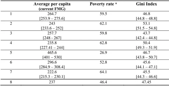
In the end, out of all the possible methodological choices, given the structure of the surveys and the data available and apart from the issue of defining aggregates, the question of whether or not the regional price differentials13 are taken into account has the greatest impact on the living standards calculations (Table 2, line 10 for Côte d’Ivoire: Table 3, line 6 for Madagascar). If these relative price differentials are taken into account, the average consumption level increases significantly, by more than 10% in both cases, and poverty rates are reduced by 7 percentage points. The effects on the global inequality levels amount to 2 points in the case of Côte d'Ivoire and to 0.8 in the case of Madagascar, but these differences are not significant. However, the fact that the relative price differentials are, or are not, taken into account may explain the difference in the inequality indicators found with our own calculations and those available in the World Development Indicators in the case of Côte d’Ivoire. Overall, fewer methodological choices have to be made for income than for consumption. Apart from the question of whether or not differences in relative prices are taken into account, which is posed for consumption and income alike, choices for calculating the income aggregate were above all concerned with the way of assessing farming income in the Ivorian case14.
Whatever the case may be, except for the questions of regional and infra-annual prices, these methodological choices do not have a great deal of impact on the form of living standards distributions. Instead, it is data entry errors and their corrections that have a significant impact on the assessment of living standards and inequalities. Nonetheless, it is quite legitimate to question whether the structure of consumption and income and the levels of inequalities produced by these surveys are realistic.
11 The per capita expenditure logarithm was regressed on the indicator for the period of the household survey, regional indicators, type of crop and level of self-consumption, checking certain features of the household such as size and level of education.
12
Subsequently, we do not take into account infra-annual inflation notably to compare more easily household data with National Accounts. 13 In the case of Côte d’Ivoire, they are far removed from reality, given that the latest regional pricesdate from 1985. On the contrary, in the case of Madagascar, the deflators used are precisely those calculated by the Madagascan Institute of Statistics when it processed the national survey (EPM) for 1993.
Table 3: Impact of methodological choices on consumption aggregate, Madagascar
Average per capita
(current FMG)
Poverty rate * Gini Index
1 264.7 [253.9 – 275.6] 59.5 46.8 [44.8 – 48.8] 2 243 [233.6 – 252] 62.1 53.1 [51.5 – 54.8] 3 257.7 [248 - 267] 59.8 43.7 [42.4 – 44.8] 4 235.8 [227.41 – 244] 62.8 50.4 [49.3 – 51.9] 5 465.6 [401 – 530] 26.9 46.7 [43.8 – 50.7] 6 296.6 [284.9 – 308.4] 52.8 45.6 [44.1 – 47.1] 7 222.6 [215.3 – 230.1] 64.1 45.5 [44.3 – 46.6] 8 237 46.4 47.45
1. Current expenditure, incl. imputed rents, transfers and consumer durables; 2. Definition n°1 without imputed rents
3. Definition n°1 without consumer durables
4. Definition n°1 without imputed rents or consumer durables
5. Definition n°1 without taking into account frequency of purchase during the year 6. Definition n°1 with regional price deflators. Definition chosen subsequently. 7. Definition n°6with infra annual price deflator.
8. Sources: Average consumption and poverty rates: http://www.worldbank.org/research/povmonitor/ Gini Indexes: World Development Indicators, World Bank, 2004.
* poverty line: 203,241 FMG equivalent to 1$ PPP 85.
Confidence interval between brackets, calculated by bootstrap; in thousands of F CFA or millions of current FMG. Sources: EPM93 Madagascar, our own calculations.
1.3.
Is the initial picture of inequalities and the structure of living standards a realistic one? 1.3.1. Structure of consumption and incomeThe structure of current consumption does appear to be typical of developing countries (cf. Table 16, Appendix B): the share of food products in total expenditure exceeds 50% on average and, as can be expected, the share of self-consumption falls with the level of total expenditure. For both countries, there is a negative relation between the food budget share and the standard of living, thus confirming Engel’s law15. However, the share of food products exceeds 50% even for the higher deciles and it is difficult to know whether the fact that self-consumption accounts for a higher share of food consumption in Madagascar than in Côte d’Ivoire (40.4% of food, i.e. 24.5% of total expenditure) stems from a methodological difference or from a real difference between the two countries.
As for the structure of incomes, it is even more difficult to assess the veracity of the survey results without referring to other sources of information such as the National Accounts (cf. infra). Whatever the case may be, the surveys gave the following results. In both countries, the share of wages increases with living standards (cf. Table 17 in Appendix B): by 8 percentage points between the first and last quartile in Madagascar and by 12 points in Côte d’Ivoire. Whereas in Madagascar, the share of farm revenues in non salary income remains stable and represents over 50% of total income whatever the level of wealth, in Côte d’Ivoire this share is halved between the first and last quartile, falling from 41% to 19%. In the latter country, the income of the first three deciles is dominated by farming activities (40% of the total), whereas this income only represents a third of the total for the middle of the distribution and less than a quarter for the last three deciles. However, an examination of the inequalities suggests that part of the results may possibly be due to measurement errors.
15 Housing is the second item of expenditure (10% of the total in Madagascar and 14% in Côte d’Ivoire). Rent accounts for 50% of housing expenditure in Madagascar and 62% in Côte d’Ivoire; this share falls more strongly with the standard of living in Madagascar than in Côte d’Ivoire. The budget share of expenditure on consumer durables, domestic care, health and leisure logically increases with wealth, once again in a more pronounced way in Madagascar.
1.3.2. Level of inequality and decomposition of inequalities by source of income
The greatest income disparities seem to be found in Côte d'Ivoire (cf. Table 4, and Table 17, Appendix B): the Gini index is higher (52.2 compared with 40.9 in Madagascar) and the ratio of last decile over first decile (d10/d1) is 35 compared with 10 for Madagascar. On the other hand, in terms of consumption, there is greater dispersion in Madagascar than in Côte d'Ivoire. In Madagascar, the fact that inequalities are greater in terms of consumption rather than income is surprising and contrary to results usually found in other countries. We can also note the low level of the highest incomes in both countries. In Côte d'Ivoire, the maximum incomes correspond to the average formal wage of a non African, whereas in Madagascar they are at the level of the average annual salary of a Madagascan senior executive working in a formal industrial company. These two observations seem to indicate that the highest incomes are under-estimated, particularly when it comes to non-salary incomes.
Table 4: Summary of differences in living standards and distribution extremes
Côte d’Ivoire (1998) Madagascar (1993) On expenditure On income On expenditure On income Current € per capita per month
Minimum 3 0 1 -27
C1 (1stcentile) 7 2 1 -0
P10 (upper bound, 1stdecile) 12 8 2 3
P90 (lower bound, 10thdecile) 103 93 20 25
C100 (last centile) 713 823 182 129
Maximum 2 249 3 697 1 504 429
Average per capita 44 48 13 16
In $ PPP 1998
Minimum 7 1 1 -32
C1 (1stcentile) 16 6 1 0
P10 (upper bound, 1st decile) 29 19 3 4
P90 (lower bound, 10th decile) 240 218 23 30
C100 (last centile) 1 669 1 926 218 154
Maximum 5 262 8 651 1 802 514
Average per capita 104 113 16 19
GDP per capita per month ($ PPA
98) 123 64 Coefficient de Gini (%) Confidence interval 43.6 [42.7 – 45.2] 52.2 [50.20 – 54.52] 47.5 [45.9 – 50.0] 40.9 [39.8 – 42.3] P90/P10 8 12 8 8
Not corrected; Confidence intervals between brackets, calculated by bootstrap. Sources: EPM93 Madagascar, ENV98 Côte d’Ivoire, our own calculations.
Although they present similarities, Madagascar and Côte d’Ivoire are different in terms of structures of income and sources of inequalities (Table 5). The most commonly used method for decomposing inequalities by source of income is the so-called “natural” method of Gini index decomposition, which adds three elements for each income component: its share in total income, its Gini index and a correlation coefficient that captures the relationship between each of the income components and its distribution16. Salaries represent 22% of total income in Madagascar and 28% in Côte d’Ivoire, whereas income from non-salary activities represents 66% and 60% respectively. However, in Madagascar, it is farming revenues which are most important (88% of income from work activity compared with only 42% in Côte d’Ivoire). Public and private salaries make relatively small contributions to global inequalities in the two countries, due to their small share in total income, and despite representing relatively high levels of inequality. In Côte d’Ivoire, inequalities in farming revenues are quite high (Gini index of 72 compared with 54 for Madagascar), but farming revenues are only responsible for 20% of total inequalities whereas their contribution exceeds 50% in Madagascar. On the contrary, income from non-farming activities makes a very low contribution to total inequalities in Madagascar (8%) whereas it contributes around 43% in Côte d’Ivoire. As this difference seems very large, a comparison must be made with other data sources in order to hone the diagnosis of the quality of the surveys.
Table 5: Decomposition of inequalities by source of income
Sources of per capita income Coefficient Gini Share of total income contribution Relative contribution Absolute Côte d’Ivoire Private salary 88.2 17.7 18.4 9.6 Public salary 95.3 7.6 8.7 4.6 Farming activities 71.9 27.5 19.8 10.3 Non-farming activities 80.9 35.2 43.8 22.9 Assets 74.4 5.8 3.8 2 Pension, insurance 98.1 1.5 1.8 0.9 Public transfers 94.5 0.7 0.6 0.3 Private transfers 92.4 2.8 1.78 0.9 Other income 97.8 1.1 1.2 0.6 Total 52.2 100 100 52.2 Madagascar Private salary 83.2 15.4 15.6 6.4 Public salary 95.5 6.8 10.6 4.3 Farming activities 54.6 58.5 52.9 21.7 Non-farming activities 90.3 7.5 8.2 3.4 Assets 57.6 5 4.2 1.7 Pension, insurance 99.2 0.08 0.08 0.03 Public transfers 98.5 1.04 1.3 0.5 Private transfers 22 1.7 1.6 0.7 Other income 93. 3.9 5.3 2.2 Total 40.9 100 100 40.9
2. COHERENCY WITH NATIONAL ACCOUNTS?
Given the differences of methods and cover17, there is clearly no real reason why the two sources of information, i.e. survey data and National Accounts aggregates, should arrive at a similar assessment of household consumption and/or income levels and in fact it is hardly surprising that this is not the case. Following work by Ravallion (2001), Deaton (2004) shows that in 277 surveys carried out throughout the world, the per capita consumption found in the surveys is underestimated compared with the National Accounts, the ratio between the two data sources averaging 86% (with a standard deviation of 31%). This average ratio amounts to 78% (standard deviation 10%) for OECD countries, although they are renowned for having better statistical resources than other countries.
It is worrying that there should be such a wide gap between the two sources and also that this gap is widening all the time, whether it be in rich countries such as the United States and Great Britain, or in developing countries. In a sample of non-OECD countries from 1990 to 2000, the growth rate of consumption found in the surveys was, on average, half of that found in the National Accounts (Deaton 2004). This confirms the diagnosis that household surveys have difficulty in capturing the top end of income distributions. This is particularly true in the case of developing countries in phases of high economic growth, such as India, where the emergence of new wealthy social classes is completely overlooked by the surveys (Banerjee and Piketty, 2003).
For the two countries studied here, the two sources of information show incoherencies, mainly in the case of Madagascar, which suggest that income (but also consumption) has been underestimated in the household survey, but also problems in the National Accounts. In the Ivorian case, despite the small amount of information that can be pieced together18, the two data sources are relatively coherent (Table 18, Appendix C). It was found that the surveys underestimated consumption by only 8%19 and
17 For a discussion on the conceptual differences in the aggregates, see Guénard and Mesplé-Somps (2004). 18 Certain elements of information are missing in the surveys, such as tax paid.
income by 16.8%20. These results are in line with averages for African countries, where gaps between the two data sources are relatively small (around 15% according to Deaton, 2004).
Data from the Madagascan survey greatly underestimates household consumption compared with national aggregates (cf. Table 18, Appendix C).21 In the end, it was only possible to match 53.5% of the National Accounts data with the survey data, with large disparities from one budget item to another. All the items are lower than the National Accounts figures, except for consumer durables and other goods.
Non-salary incomes are four times higher in the survey than in the National Accounts (cf. Table 19, Appendix C). Salaries, on the contrary, are lower by half. These differences in the shares of salaries and self-employment incomes in total household income may be due to differing definitions, as the sum of the two is almost identical. Income drawn by entrepreneurs in quasi-corporate undertakings represents over 50% of Madagascan households’ available income in the National Accounts, which seems very high in absolute terms and also compared with the survey, which puts it at about 10%. This gap alone accounts for the entire difference between the figures for total income in the National Accounts and in the survey.
Data from the National Accounts is generally used to correct data from household consumption surveys. In this case, the consumption in the surveys is adjusted using an average coefficient taken from the National Accounts, following the example of Bourguignon and Morrisson (2002) and Sala-i-Martin (2002). This method implies, on the one hand, that the National Accounts are considered to be more reliable than the surveys and, on the other, that the gap between the two sources is neutral in distributive terms, i.e. that the underestimation of consumption in the surveys is a constant proportion, at all levels of wealth. As we find these assumptions debatable, this method has not been used in this study.
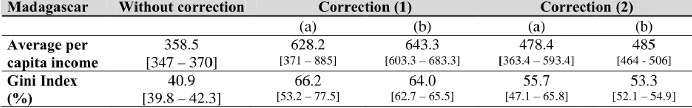
However, we did think it worthwhile to try to correct the survey data on income, even if the income drawn by formal entrepreneurs in Madagascar is quite probably overestimated in the National Accounts. In order to do this, the first step was to identify these formal entrepreneurs in the survey. This was not an easy task, because the section of the questionnaire dealing with employment did not contain the modality “corporate or quasi-corporate entrepreneur”. Twenty-two individuals declared themselves as “employers”, including 14 who owned a company with a “statistical identity card”. In the absence of more precise information to be able to check whether these are corporations or quasi-corporations, these individuals were put in the same category as formal entrepreneurs, 10 of which are in the last two consumption deciles. In addition, 4% of the households surveyed declared that they had received “dividends and other business revenues”, 50% of which were distributed in the three most wealthy deciles.
Four simulations are proposed (cf. Table 6). The first two help equalize the income of formal entrepreneurs in the survey with that of the National Accounts. 90% of the income given in the National Accounts is either allocated exclusively to formal entrepreneurs, or to the latter in addition to households receiving dividends. In this case, the average per capita income increases by around 50% and inequalities increase by over 23 points. The two remaining simulations allocate only 40% of the income given in the National Accounts, in the same way as for the previous two simulations. This re-estimate was made equiproportionally to the income from non-salary, non-farming activities and income received in the form of dividends. In this case, inequalities increase by over 15 points, and the Gini coefficient increases by 12 points when the transfer of dividends concerns formal entrepreneurs and households receiving dividends. Income inequalities are then higher than consumption inequalities.
20 Survey data was therefore used to compile the household account in the National Accounts.
21 Problems were encountered for matching the two types of information, particularly for aggregating household expenditure on consumption and for harmonising branch and product nomenclatures for surveys and Input-Output Tables. For details on matching the two data sources, see Guénard and Mesplé-Somps (2004).
Table 6: Correction of Madagascan survey data using National Accounts
Madagascar Without correction Correction (1) Correction (2)
(a) (b) (a) (b) Average per capita income 358.5 [347 – 370] 628.2 [371 – 885] 643.3 [603.3 – 683.3] 478.4 [363.4 – 593.4] 485 [464 - 506] Gini Index (%) [39.8 – 42.3] 40.9 66.2 [53.2 – 77.5] 64.0 [62.7 – 65.5] 55.7 [47.1 – 65.8] 53.3 [52.1 – 54.9] Correction (1): Addition of 90% of income drawn by entrepreneurs in quasi-corporate undertakings given in the National Accounts Correction (2): Addition of 40% of income drawn by entrepreneurs in quasi-corporate undertakings given in the National Accounts To « formal » entrepreneurs
To « formal » entrepreneurs and households declaring receipt of dividends
Confidence intervals between brackets, calculated by bootstrap; in thousands of F CFA or millions of current FMG Sources: EPM93 Madagascar; our own calculations.
In the case of India, Banerjee and Piketty (2003) use a different method to try to make up for the difference between the National Accounts and the household surveys. They re-estimate the high incomes from surveys between 1956 and 1998 using tax data and a method already developed for France and the United States (Piketty, 2003; Piketty and Saez, 2003). Their corrections highlight a 50% growth in income for the last centile and a tripling of average income for the last centile. The gap between the national data and the survey data is only partly reduced and explained by the fact that the latter are not well suited to capturing the income of wealthy individuals. The work using tax statements is extremely interesting, but for want of such information, we were unable to apply it to our case.
3. ASSESSMENT AND MEANS OF CORRECTING SAMPLE BIASES
3.1.
Survey cover and potential biasesIn order to measure the distributive impact of any sample biases of the surveys, we compared elements from the sample design with population censuses conducted in 1998 in Côte d'Ivoire (RGP98) and 1993 in Madagascar (RGP93) calculating several indicators: rate of urbanisation, structure by nationality, by ethnic group, by socio-professional group, by level of education and by type of housing, depending on the information available in each of the countries. In Côte d'Ivoire, the sample design for the 1998 survey was made on the basis of the 1988 General Population Census, which is problematical. In Madagascar, however, the survey is based on a census in the same year, 1993 (INSTAT, 1997).
A first potential bias concerning the possible under-representation of what are in principle the poorest households, i.e. households with no fixed abode, could not be evaluated. The census in Madagascar specifies that this specific population was interviewed separately and independently from the “domiciled” population, but we do not have the results in question. In Côte d’Ivoire, the definition of a household used in the successive censuses (1975, 1988, 1998) takes into account the place of residence22. In practice this means that homeless households were neither covered by the census nor by the surveys. On the contrary, other significant sample biases were identified:
- The rate of urbanisation is significantly overestimated in the survey (45%) compared with the census (42%); more precisely, Abidjan accounts for 21% in the survey and only 19% in the census.23 This confirms the fact that urban growth is overestimated in many countries, particularly in Africa (Bocquier, 2004) while it seems to be decreasing in Côte d’Ivoire (Beauchemin, 2004);
22
“According to the General Population and Housing Census of 1998, the ordinary household is composed of a group of related or unrelated people who recognize the authority of a single individual called the “head of household”, living under the same roof or in the same concession and whose resources are pooled or partly so.” (Touré, 2001).
23 The differences between the survey and the census are significant as confidence intervals for the percentages of urban population and Abidjan population are [44.2 % – 48 %] and [20.3 % – 22.7 %] respectively.
- The population of foreigners of African origin is under-represented; it accounts for 17% of the total population in the survey compared with 26% in the census.24 This bias points to an underestimation of inequalities given that these foreigners are more likely to belong to the bottom of the distribution, as demonstrated by Grimm et al. (2002);
- Households living in villas or individual houses are significantly underestimated in the survey (22% compared with 39% in the census) and this is also the case for households in makeshift housing such as shacks or huts (6% compared with 11%), particularly in urban areas. This bias points to a potential underestimate of inequalities due to a poor assessment of the distribution extremes.
In the Madagascan case, the corrections concerned geographical strata (urban or rural area) by region and by level of education (cf. correction 1 and 2 of Table 7). The rate of urbanisation for the survey is 18.5%25 compared with 22.9% in the census. In terms of education, 48.2% of individuals in the survey have received no education compared with 33.7% in the census and 39% have been educated to primary level compared with 47% in the census26. No clearly identified bias could be extracted from the other indicators available, particularly on housing characteristics (type of lighting, fuel used for cooking, type of floor, etc.). In addition, the breakdown of the population covered by the census by type of housing is not available.
In both countries, another bias is likely to have a strong impact on living standards and their distribution, namely foreigners of non-African origin residing in the country. This small population was deliberately not accounted for in the surveys. In Côte d'Ivoire, this concerned 32,700 individuals (source RGP98), mainly expatriate Europeans (16,028) and persons of Lebanese origin, i.e. 0.2% of the country’s total population, a very marginal percentage in demographical terms with no possible comparison to its economic weight. In Madagascar, the foreign population was not covered by the survey either. It represents 0.2% of total population : over a third are Europeans, 29% Asians, 10% Africans, 17% from the Indian Ocean and the remainder from the United States, the former USSR, Oceania and stateless persons (INSTAT, 1997).
3.2.
Impact of correction of biases on inequality levelsThe corrections consisted in restratifying the survey a posteriori by an iterative correction process of cross-tabulation for two criteria (nationality/geographical stratum, for instance). The households’ relative weights could then be corrected by a coefficient restoring their share in the total population before proceeding with the aggregation of incomes.
Three weighting corrections were made for Côte d’Ivoire: the first for ethnic origin and nationality by geographical stratum (correction 1), the second by type of housing by geographical stratum (correction 2) and the third by nationality by type of housing (correction 3), to correct levels of consumption and income (cf. Table 7). None of these corrections has a significant impact on income or consumption inequalities (cf. Table 7).
For Madagascar, the impact on the Gini coefficient is also fairly low, amounting to roughly one Gini point, and therefore non significant. These small impacts on inequalities no doubt stem from the method itself, as it amounts to replacing the missing values in the sample with average values for the corresponding sub-populations. There is therefore the implicit assumption that the non-respondents in a category (or the non-interviewed, which comes to the same thing) cannot be distinguished on average from the respondents. It also artificially introduces a concentration around the average values, meaning that the variances are calculated on the adjusted sample that underestimates the real differences.
24 This difference is also highly significant since the confidence interval for the percentage of foreigners of African origin in the population surveyed is [16.9 % – 17.9 %];
25 The confidence interval is [17.98% – 18.91%]
These results suggest that the real biases are not to be found in the sample designs, even though these are not perfect as in the case of Côte d’Ivoire, but from an underestimate of certain types of income, as we mentioned above. We therefore adopted a different method for adding the foreign population. For Côte d’Ivoire, we could have corrected this bias by correcting the weight of households living in villas or flats in urban areas, as these types of housing are partly occupied by Europeans and Lebanese. This would amount to assuming that this population has the same living standards as the African households living in this type of housing and covered by the survey. However, non-Africans tend to receive income in line with levels in their countries of origin. We therefore drew up two hypotheses. The first, so-called “high” hypothesis27, assumes that this population, comprising households with four members on average, has a monthly income of 4,500 euros per household and consumes on average 2,290 euros per month per household (in this case, their consumption level is equivalent to that of the ten most wealthy households). A second, so-called “low hypothesis”, consists in allocating them with the average income of French households (approximately 2,100 euros) and average consumption of around 1,100 euros28. Whereas the average consumption and income levels rise by 15% and 30% with the high hypothesis, and 7% and 11% with the low hypothesis, Gini indexes on expenditure rise by 6 points and on income by 9 points with the high hypothesis and by 2 points and 4 points with the low hypothesis (cf. correction 4, Table 7).
In Madagascar, given the make-up of the foreign population, we assumed that one third of them have living standards equivalent to Western expatriates, and that the remaining two-thirds have living standards equivalent to the country’s average. As in the case of Côte d’Ivoire, the high hypothesis for the income of the population from Northern countries has a very strong impact (cf. correction 4, Table 7): average consumption and income levels rise by 12 and 15% respectively, whereas the Gini coefficient on consumption increases by 6 points and that of income by 8 points. With the low hypothesis, all these effects are halved. Hence, even though the results of this simulation exercise on inequalities are sensitive to the chosen hypotheses, they show the extent to which inequalities can be underestimated if this category of households is not taken into account.
Table 7: Adjustment of consumption and income levels by correcting sample design
Without adjustment Correction 1 Correction 2 Correction 3 Correction 4
Côte d’Ivoire (1) (2)
Ave. per capita
consumption [337 – 360] 349 347 [336 – 359] 347 [332 – 363] 336 [322 – 350] 403 [372 – 434] 373 [356 - 390] Gini Index (%) 43.6 [42.1 – 45.2] 43.6 [42.3 – 45.5] 44.2 [42.3 – 46.7] 43.7 [41.7 – 45.3] 50.0 [47.4 – 53.3] 46.2 [44.3 – 48.0] Ave. per capita
income [359 – 402] 381 385 [362 – 408] 387 [361 – 414] 382 [356 – 408] 491 [427 – 554] 426 [393 – 458] Gini Index (%) 52.2 [50.3 – 55.6] 52.5 [50.3 – 54.3] 52.9 [50.7 – 56.0] 52.8 [50.1 – 55.2] 61.8 [56.6 – 66.1] 56.2 [54.0 - 58.8] Madagascar
Ave. per capita consumption 297 [285 – 308] 307 [295 – 320] 311 [298 – 324] 332 [295 - 369] 314 [293 – 335] Gini Index (%) 45.6 [44.1 – 47.1] 46.4 [44.9 – 48.5] 46.1 [44.6 – 47.9] 51.3 [47.4 – 56.5] 48.5 [46.4 - 51.7] Ave. per capita
income 359 [347 – 370] 362 [350 – 373] 366 [353 – 378] 412 [358 – 465] 385 [357 – 414] Gini Index (%) 40.9 [39.8 – 42.3] 41.3 [40.1 – 43.0] 41.1 [39.6- 42.5] 48.5 [40.6 – 53.4] 44.9 [41.2 - 49.4] In thousands of F CFA or millions of current FMG; confidence intervals for Gini coefficients between brackets, calculated by bootstrap.
Correction 1: on ethnic origin and nationality by geographical strata in Côte d’Ivoire and on area of residence and geographical strata in Madagascar.
Correction 2: on the type of housing by geographical strata in Côte d’Ivoire and on levels of education by geographical strata in Madagascar. Correction 3: by nationality and type of housing in Côte d'Ivoire.
Correction 4: addition of foreign population of non-African origin in Côte d'Ivoire and the foreign population in Madagascar, with high hypothesis (1) and low hypothesis (2) of living standards for populations of non-African origin.
Sources: EPM93 Madagascar, ENV98 Côte d’Ivoire, our own calculations.
27
Given that the average non-African salary in the private sector was approximately 2,600 euros in 1996 (Cogneau and Mesplé-Somps, 2002). However, expatriates’ salaries in the public sector are far higher than this average private salary (approximately 6,000 euros) and it can also be assumed that their spouses also receive an income.
28 This covers households which declare a positive or nil income to the tax authorities and for which the reference person is neither a student nor doing national service (source INSEE).
In the following section, we continue our discussion on measurement errors by examining under-declarations of income. Apart from comparisons with the National Accounts and methods for rectifying sample design, with the advantages and limits given above, several methods have been used by the community of researchers and statisticians to rectify biases from under-declarations and non-responses on income. After showing the incoherency of consumption and income declarations using residual savings rates calculations, we will apply different methods of adjustment to the two surveys studied here.
4. Under-declarations and non-responses
4.1.
Incoherencies between income and consumption declarationsIt is a well known fact that surveys generally provide negative savings rates and there are discussions as to the origin of this phenomenon. As Deaton noted (1997, p369): “household surveys from
developing countries frequently do record dissaving by substantial fractions of households. There is no doubt that some of this is due to underestimation of income relative to consumption, but the observation may have more truth to it than is often credited”. However, the fact that large numbers of
households had levels of income representing half of the declared levels of consumption attracted our attention (cf. Table 8) and seems to suggest that there are large problems with under-declarations of income, throughout the distribution in Côte d’Ivoire and at the top of the distribution only in Madagascar.
In Côte d’Ivoire, the average rate of residual savings is -86%, and is always negative, whatever the consumption decile, and decreases with the level of consumption. Thus, 61% of households in the Ivorian sample have negative residual savings, which can be normal behaviour in the event of loss of employment, no harvest or other negative shocks. However, over 20% of households had a residual savings rate lower or equal to -100%. These cases are found throughout the distribution, but more frequently in the highest deciles. We tested to see whether there was a link between the economic difficulties experienced by the households and the behaviour adopted to face up to them (using their savings, selling off assets, getting into debt), but found that households with the highest rates of dissaving did not have to face any greater economic difficulties than the other households.
In Madagascar, the average rate of residual savings is only -4% and is distributed in a completely different way: the average savings rates are positive and relatively high for the entire distribution with the exception of deciles 3, 9 and 10. Only 5% of the households in the total sample consumed twice more than their current income allowed them to. It is also surprising to note such high savings rates at the bottom of the distribution, which seems to suggest that consumption is underestimated.
Table 8: Average residual savings by consumption decile
Côte d’Ivoire Madagascar
Consump-tion decile Average savings rate (%) Stand. Devia- tion % of households with savings rates
≤ -100% Average savings rate (en %) Stand. Devia- tion % of households with savings rates
≤ -100% 1 -7.7 84.7 7 32.5 30.9 0 2 -50.6 533.5 11 25.6 91.6 2 3 -43.7 244.8 11 -32.5 1199 2 4 -39.5 147.6 17 27.4 46.3 2 5 -60.5 250.3 15 20.5 126.2 2 6 -62.8 214.1 21 11.1 105.4 4 7 -55.9 153.5 22 14.3 467.5 4 8 -77.3 196.8 26 4.9 98.6 4 9 -125.6 366.6 37 -19.9 194.4 9 10 -337.2 1910.2 52 -125.9 1948.6 18 Total -85.9 662.8 22 -4.2 745.2 5
In order to make the income declarations coherent with the consumption declarations, even though these, too, are subject to errors, we then attempted to rectify the income declarations using the different methods currently available.
4.2.
Correction of biases for under-declarations of income and for non-responses, and comparison with other data sourcesWe propose several adjustments: a correction based on the information concerning declared savings (Madagascar); a correction for missing values by Rubin’s multiple imputation method (Rubin 2004); and finally, using information given in the Balances of Payments, an assessment of capital flight attributed to certain households in the survey which are likely to hide part of their income.
4.2.1. Adjustment with declared savings
A first method that Loisy (1999) implemented in France helps adjust the income by using information on the amounts of accumulated savings declared by the households. Only the EPM93 survey in Madagascar asked the households about the flow of savings accumulated during the current year, and on credits contracted. In line with Loisy (1999), income can be adjusted as follows: in the cases where the sum of declared consumption and savings (C + Sdeclared) is higher than the declared income
(Ydeclared), and the household has not obtained a consumption loan, the income can be replaced by (C +
Sdeclared); in the other cases, i.e. where the income is higher than (C + Sdeclared) and when the households
have a lower income but have obtained a loan for the purchase of consumer goods, no replacements are made. This adjustment concerned 23% of the Madagascan households29.
Table 9: Adjustment of Madagascan income with declared savings
Without adjustment With adjustment by declared savings Per capita income 358.5
[347– 370] 407.8 [393 – 422.6] Gini index (%) 40.9 [39.8 – 42.3] 42.9 [41.34 – 44.36]
Average residual savings rates by consumption decile (%)
1 32.5 35.9 2 25.6 35.1 3 -32.5 33.2 4 27.4 33.5 5 20.5 30.5 6 11.1 26.6 7 14.3 22.8 8 4.9 21.9 9 -19.9 17.8 10 -125.9 7.8 Total -4.2 26.5
Confidence intervals between brackets, calculated by bootstrap; in thousands of F CFA or millions of current FMG. Sources: EPM93 Madagascar, ENV98 Côte d’Ivoire, our own calculations.
This correction increases the average income by 14%, the average residual savings rate by 30 percentage points and the Gini index by 2 points (gap not significant). The total savings rate for Madagascan households is then 27%, a relatively high rate compared with the National Accounts, which give a rate of only 2.3%. This method does not appear to be entirely satisfactory given that it does not obtain a Gini coefficient on income higher than that on consumption.
29 45% in the French « Family Budget 1995 ». Contrary to Loisy, we do not correct the consumption declarations beforehand for the differences observed compared with the National Accounts, for the reasons stated above..
4.2.2. Accounting for missing values Basic principles:
A high percentage of households can refuse to answer the part of questionnaires that concerns their income. For example, in the case of the American Current Population Survey, the rate of non-response exceeded 25% at the beginning of the 1980s (Lillard et al., 1986). The community of survey statisticians proposes several ways of accounting for missing values. Although this problem concerns less than 1% of the sample in the two cases studied here (cf. note 6)30, it is nonetheless interesting, in our view, to examine the different adjustment methods proposed, to see how they could be used to correct under-evaluations of income, a problem that we identified as important in our previous diagnoses. The following paragraphs outline the basic principles of some of the methods for adjusting missing values.
One relatively simple correction is to allocate the average or median31 of observations belonging to the “same category” as the missing observation, in what is called the mean or median imputation method. This method is used by the American Bureau of Statistics to make up for missing values on income: biases for non-responses in income declarations are corrected by allocating to individuals who refused or omitted to declare their income the average response for households with the same characteristics in terms of age, race, gender, type of occupation, level of education and number of hours worked (Census Bureau, 2002). This procedure is not perfect, as the distribution of the new variable is incorrect because average values have been added. This means that variance is underestimated, thereby artificially increasing the significance of the regression estimators. In addition, this matching method does not allow for a large number of variables to be taken into account.
A second correction consists in estimating an explanatory model for the variable for which part of the observations are missing, using predicted coefficients to estimate the missing values, in what is called the imputation using a prediction model. Székely and Hilgert (1999) adopted this method in several Latin American countries, estimating income for each income component and classifying the households according to predicted income. Households which did not provide information on their income were allocated a predicted income, plus a residual term equal to the average of the error terms for the two households just above and just below it in the new distribution.
This method, like the preceding one, does not take into account the selection mechanism which prevails in the total or partial non-response. And yet, for data on income, several elements suggest that not only the fact of being surveyed may not be random (problem of sample bias mentioned above), but also, the fact of answering the interviewer’s questions on income correctly or not may not be random either. As we already suspected, missing or underestimated income in the surveys studied are related to income from assets or non-salary activities. In addition, it can be assumed that, from discretion or fear that the information given to the interviewer will be passed on to the tax authorities, certain households refuse to declare their income over a certain amount.
There are several possible mechanisms governing the process of non-response or partial response (Rubin, 2004). A selection mechanism is Missing Completely at Random (MCAR) when the probability of a given variable X being missing does not depend on any observed variable. This hypothesis is often quite unrealistic. The Missing at Random (MAR) selection is a slightly less restrictive hypothesis. The probability of answering the questionnaire depends on part of or all the values observed (data collected in the survey or data coming from the survey design) but is independent from the behaviour model – in the present case, the model of income formation. In cases where the probability of not being included in the data depends on these same missing observations and that the two models, of selection and of behaviour, are not independent, the process of missing values is said to be “non-ignorable”. In cases where the respondent is informed of the object of the survey, which is the case of household surveys in developing countries, it is possible that the selection process is endogenous and that there is no variable that allows selection to be ignored (Gautier, 2005).
30 General practice in this case is to eliminate observations for which certain variables are missing (case deletion). 31 The median is preferred to the mean when the latter is too dependent on the values at the extremes of the distribution..