Financial Development and Growth:
A Re-Examination using a Panel Granger Causality Test
Christophe Hurlin and Baptiste Venety
August 2008
Abstract
In this paper we investigate the causal relationship between …nancial develop-ment and economic growth. We use an innovative econometric method which is based on a panel test of the Granger non causality hypothesis. We implement various tests with a sample of 63 industrial and developing countries over the 1960-1995 and 1960-2000 periods. We use three standard indicators of …nancial development. The results provide support for a robust causality relationship from economic growth to the …nancial development. On the contrary, the non causality hypothesis from …nancial development indicators to economic growth can not be rejected in most of the cases. However, these results only imply that, if such a relationship exists, it can not be easily identi…ed in a simply bi-variate Granger causality test.
Keywords: Granger Causality Tests; Panel Data; Financial Development; Eco-nomic Growth .
JEL classi…cation: C23; C11; O16; G18; G28
LEO, University of Orléans. Rue de Blois. BP 6739. 45067 Orléans Cedex 2. France. E-mail address: christophe.hurlin@univ-orleans.fr.
1
Introduction
Following McKinnon (1973) and Shaw (1973), a very large literature tries to assess
the nature of the relationship between …nancial development and economic growth.
But, it seems that “economists hold di¤erent views on the existence and direction of
causality”in this context (Al-Yousif, 2002). As it was mentioned by Patrick (1966), the
both directions of causality between the two variables can be considered as potentially
valid. On the one hand, …nancial deepening may promote economic growth. This
approach, called the supply-leading hypothesis, assumes that the optimal allocation of
resources results from the …nancial system development. On the other hand, growth
can also promote the development of the domestic …nancial system. This is the
demand-following approach. It assumes that economic growth leads to an increasing demand for
…nancial services which promotes …nancial development: in that case, …nancial system
is supposed to respond passively to economic growth. Besides, a third approach can be
considered in which the two variables are mutually causal. Naturally, the direction of
causality is crucial for the choice of the development strategy: “one could argue that,
only in the case of supply-leading, policies should aim to …nancial sector liberalization;
whereas in the case of demand-following, more emphasis should be placed on other
growth-enhancing policies” (Calderon and Liu, 2003, p. 331).
In the same time, empirical studies have generally failed to clearly identify the
Roubini and Sala-i-Martin (1995) as well as King and Levine (1993a,b), De
Grego-rio and Guidotti (1995), Levine et al. (2000) or Calderon and Liu (2003) support the
supply-leading hypothesis whereas Jung (1986) supports the second way of causality and
Demetriades and Hussein (1996) or Greenwood and Smith (1997) …nd a bidirectional
causality. Following Al-Yousif (2002), one can consider that the empirical literature on
that question is still “mixed and inconclusive”and that the causal relationship between
…nancial development and economic growth remains unclear. That is why we propose
a re-examination of this issue using an original panel data approach.
Our methodology is based on the panel non causality test developed by Hurlin (2005,
2007). It consists in a simple test of the Granger (1969) non causality hypothesis in a
heterogeneous panel model. The use of a panel data methodology in this context can
be justi…ed by the same arguments as those used in the contemporary panel unit root
tests literature. The …rst one is the power de…ciencies of the pure time series-based
tests of non causality in short sample. The second is the possibility to consider an
heterogeneous model to test the non causality hypothesis. As it is the case for the
panel unit root tests, the model used in this paper is speci…c to each country of the
sample: the only common feature of the sample is assumed to be the null hypothesis of
non causality. So, it is possible to test the relationship between economic growth and
…nancial development without considering the same dynamic model for all the countries
of the sample. It allows taking into account the heterogeneity of this relationship not
only between developed and developing countries for instance, but also between the
Indeed, one of the main issues of a panel Granger causality test is the heterogeneity
of the model and of the causality relationship. Let us assume for instance that we test
the non causality from …nancial development (represented by a variable x); to growth
(represented by a variable y). For each country; we say that …nancial development
measure (x) is causing growth (y) if we are better able to predict growth using all
available information than if the information apart from x had been used (Granger,
1969). But, when growth and …nancial development are observed on N countries,
the issue consists in determining the optimal information set used to forecast y: Several
solutions could be adopted. The most general is to test the causality from the variable x
(…nancial development) observed on the ithcountry to the variable y (growth) observed
for the jth country, with j = i or j 6= i: It implies that we can identify a causality
relationship when the past values of the …nancial development indicator for France give
an information about the future values of growth for Japan. In this paper, we use a
more restrictive solution derived from the time series analysis. We say that there is
causality from …nancial development to growth if and only if, the past values of the
variable x observed on the ith country improve the forecasts of growth for this country
i only. The cross sectional information is then only used to improve the speci…cation
of the model and the power of tests as in unit root test literature. In this context, we
propose to distinguish between the heterogeneity of the model and the heterogeneity of
the causal relationships from x to y. Indeed, the model may be di¤erent from an country
to another, whereas there exists a causal relationship from x to y for all countries. On
The structure of our test is similar to those used in the literature devoted to the panel
unit tests. Under the null hypothesis, we assume that there is no causal relationship
from x to y for all the countries of the panel. We call this hypothesis the Homogeneous
Non Causality (HNC) hypothesis. Under the alternative hypothesis, there exists a
causal relationships from x to y for at least one country of the sample.
The approach used is then similar to that used by Im, Pesaran and Shin (2003)
to test the unit root hypothesis. Our statistic of test is simply de…ned as the
cross-sectional average of individual Wald statistics de…ned to test the Granger non Causality
hypothesis for each country. under the assumption that the innovations of the model are
cross-sectionally independent, Hurlin (2007) show that the average statistic sequentially
converges to a normal distribution (under the HNC hypothesis) when T tends to in…nity
…rst and N then tends to in…nity. Two standardized statistics are then proposed: the
…rst is based on the exact moments of the asymptotic moments of the individual Wald
statistics, the second one is based on approximated moments for …nite T samples. This
last statistic is particularly suitable for the samples of developing countries, as in our
case.
We use a sample of 63 industrial and developing countries over the periods
1960-1995 and 1960-2000. In order to assess the sensitivity of our results to the measure of
…nancial development, we consider three indicators as in the seminal paper of Levine
et al. (2000). There are two major …ndings in the paper. First, the homogenous non
This result is robust to (i) the lag-order considered in the autoregressive model, (ii)
to the period studied and (iii) to the indicator of …nancial development used. Similar
results are obtained when the panel is split into two groups: 28 developed countries
and 35 developing countries. It suggests that this …rst causal relationship
(demand-following hypothesis) can be robustly identi…ed through a simple bi-variate Granger
causality test. On the contrary, the supply-side hypothesis is more di¢ cult to identify
with such an approach, even for developed countries. We reject the homogenous non
causality hypothesis for the total panel (63 countries) only for some lag-orders, but
these results are not robust to the choice of the proxi used to measure the …nancial
development. Besides, when only developing countries are considered the homogenous
non causality hypothesis is generally not rejected. These conclusions do not imply that
the …nancial development has no e¤ect on the economic growth. It only indicates that
if such a relationship exists it can not be identi…ed in a simple bi-variate causality
approach.
The rest of the paper is organized as follows. Section 2 brie‡y presents the
method-ology of the panel test of the Granger non causality hypothesis. Data and measure of
…nancial development are presented in section 3. Section 4 presents the results. Then
2
A panel test of the Granger Non Causality Hypothesis
We now brie‡y present our methodology based on a panel Granger non causality test
developed by Hurlin (2005, 2007). Let us consider a covariance stationary variable,
denoted x; as an indicator of …nancial development and let us denote y the GDP growth.
Both variables are observed on T periods and on N countries. For each country i at
time t; we consider the following heterogeneous autoregressive model:
yi;t= i+ K X k=1 (k) i yi;t k+ K X k=1 (k) i xi;t k+ "i;t (1)
with i = (1)i ; :::; (K)i 0: Individual e¤ects i are assumed to be …xed. We assume
that the lag-order K is common1. The autoregressive parameters (k)i and the regression
coe¢ cients slopes (k)i di¤er across countries. However, contrary to Weinhold (1996)
or Nair-Reichert and Weinhold (2001), parameters (k)i and (k)i are constant. It is
important to note that our model is not a random coe¢ cient model as in Swamy
(1970): it is a …xed coe¢ cients model with …xed individual e¤ects. For each country
the innovations "i;tare i:i:d: 0; 2";i and they are independently distributed across
groups.
Given this heterogeneous panel model, we propose to test the Homogenous Non
Causality (HNC) from …nancial development to growth as follows:
H0: i= 0 8i = 1; ::N (2)
with i = (1)i ; :::; (K)i 0: Under the alternative hypothesis, there is a causality
re-lationship from …nancial development to growth for at least one country. We allow
1
Wwill propose a sensitivity analysis on this parameter. We prefer this approach rather than using some criteria information for each individual equation with a small sample T:
for some, but not all, of the individual vectors to be equal to 0. In other words, we
assume that there are N1 < N countries with no causality from …nancial development
to growth:
H1 : i = 0 8i = 1; ::; N1 (3)
i 6= 0 8i = N1+ 1; N1+ 2; ::; N
where N1 is unknown but satis…es the condition 0 N1=N < 1: The structure of the
test is similar to the unit root test in heterogeneous panels proposed by Im, Pesaran
and Shin (2003). In our context, if the null is accepted …nancial development (variable
x) does not Granger cause growth (variable y) for all the countries of the panel. On the
contrary, let us assume that the HNC is rejected. Two cases have to be distinguished:
if N1 = 0; there is Granger causality relationship from …nancial development to growth
for all the countries of the panel. In this case we get an homogenous result as far as
causality is concerned, even if the model used is heterogeneous. On the contrary, if
N1 > 0; then the causality relationships is heterogeneous: there is no causality for N1
countries and there is causality for N N1 countries.
The test statistic is simply de…ned as the average of individual Wald statistics
associated to the test of the non causality hypothesis for the countries i = 1; ::; N . Let
WN;THnc be this average statistic.
WN;THnc= 1 N N X i=1 Wi;T (4)
where Wi;T denotes the individual Wald statistics for the ith country associated to the
statistic converges to a chi-squared distribution with K degrees of freedom. Besides,
under the assumption of cross sectional independence, these N statistics are
indepen-dent. So, the cross section average WHnc
N;T converges toward a normal distribution when
T tends to in…nity and then N tends to in…nity (see Hurlin 2007 for more details). Let
ZN;THnc be the corresponding standardized statistic.
ZN;THnc= r N 2K W Hnc N;T K d ! T;N !1N (0; 1) (5)
where T; N ! 1 denotes the fact that T ! 1 …rst and then N ! 1: For a large
N and T sample, if the realization of the standardized statistic ZN;THnc is superior in
absolute mean to the normal corresponding critical value for a given level of risk, the
homogeneous non causality (HN C) hypothesis is rejected.
However, this convergence result can not be achieved for a small T dimension.
In this case, individual Wald statistics Wi;T do not converge toward an identical
chi-squared distribution. So, we use an approximation of the two …rst moments of
their unknown distribution. This approximation is based on corresponding moments
of a Fisher distribution. Given the restrictions of our model, this distribution is a
F (K; T 2K 1). Indeed it is well known that in a dynamic model the F
distribu-tion can be used as an approximadistribu-tion of the true distribudistribu-tion of the statistic Wi;T=K
for a small T sample. Given these approximations, we propose to compute an
approxi-mated standardized statistic eZN;THnc for the average Wald average statistic WN;THnc of the
HN C hypothesis. e ZN;THnc= p NhWN;THnc N 1PNi=1E (Wi;T) i q N 1PN i=1V ar (Wi;T) (6)
where N 1 N X i=1 E (Wi;T) ' K (T 2K 1) (T 2K 3) (7) N 1 N X i=1 V ar (Wi;T) ' 2K (T 2K 1)2 (T K 3) (T 2K 3)2 (T 2K 5) (8) For a large N sample, under the HNC hypothesis, we assume that the statistic eZN;THnc
follows approximately the same distribution as the standardized average Wald statistic
ZHnc
N;T (see Hurlin, 2007 for more details).
e
ZN;THnc d!
N !1N (0; 1) (9)
The HN C test is built as follows. For each individual of the panel, we compute the
standard Wald statistics Wi;T associated to the individual hypothesis H0;i : i = 0
with i 2 RK Given these N realizations, we get a realization of the average Wald
statistic WN;THnc: Given the formula (6) we compute the realization of the approximated
standardized statistic eZN;THncfor the T and K values: For a large N sample, if the value
of eZN;THnc is superior in absolute mean to the normal corresponding critical value for a
given level of risk, the homogeneous non causality (HN C) hypothesis is rejected.
When the panel used is unbalanced, these formula can be adjusted as follows:
1 N N X i=1 E (Wi;T) ' K N X i=1 (Ti 2K 1) (Ti 2K 3) (10) 1 N N X i=1 V ar (Wi;T) ' 2K N X i=1 (Ti 2K 1)2 (Ti K 3) (Ti 2K 3)2 (Ti 2K 5) (11)
What is the main advantage of this Granger non causality panel test? For instance,
let us assume that there is no causality from …nancial development to growth for all the
N countries. Given the Wald statistics properties in small sample, the analysis based
on N individual tests is likely to be inconclusive. With a small T sample, some of the
realizations of the individual Wald statistics are likely to be superior to the
asymp-totic critical values of the chi-square distribution. These ”large” values of individual
statistics lead to wrongly reject the null hypothesis of non causality for at least some
countries. The conclusions are then no clear cut. On the contrary, in our panel average
statistic, these ”large” values of individual Wald statistics are crushed by the others
which converge in probability to zero. When N tends to in…nity, the cross-sectional
average is likely to converge to zero. The null hypothesis of homogeneous non
causal-ity hypothesis will not be rejected. In this sense, our testing procedure may be more
restrictive and may result in more clear-cut conclusions as compared to those obtained
with pure time series tests.
3
Data and measures of …nancial development
We consider three unbalanced panels: the …rst one includes 63 industrial and developing
countries, the second one corresponds to 35 developing countries and the last includes
28 developed countries. The countries considered in this study are globally the same
as those considered in Levine et al. (2000) or Calderon and Liu (2003), given the data
availability (see appendix A). We consider two periods: the …rst one (1960-1995) is the
same as Levine et al. (2000) and the second one (1960-2000) includes the end of 90s.
our heterogeneous approach. Finally, for each panel we use three di¤erent measures of
…nancial development which were elaborated by Levine et al. (2000).
BANCRED: Private credit by deposit money banks to GDP calculated using
the following de‡ation method:
f(0:5) [Ft=Pte+ Ft 1=Pt 1e ]g=[GDPt=Pta] (12)
where F denotes credit by deposit money banks to the private sector (line 22d),
GDP denotes gross domestic product (line 99b), Pe is end-of period consumer
price index (line 64) and Pa is the average consumer price index for the year.
This …rst measure isolates credits issued to the private sector as opposed to credits
issued to the public sector.
PRIVCRED: This indicator is calculated according the formula (equation 12),
where F denotes the credit by deposit money banks and other …nancial
institu-tions to the private sector (lines 22d + 42d). PRIVCRED is the preferred Levine
et al. (2000) …nancial development indicator .
LIQLIAB: Liquid liabilities of the …nancial system (currency plus demand and
interest-bearing liabilities of banks and non-bank …nancial intermediaries) to
GDP, calculated using the same de‡ation method (equation 12) where F denotes
liquid liabilities (line 55l).
These three indicators address the stock-‡ow problem of …nancial intermediary
bal-ance sheets items being measured at the end of the year, whereas nominal GDP is
measured over the year2 . The economic growth indicator is the real GDP per capita
(PIBR) (growth and log levels). It is taken from the Penn World Tables 6.1. All the
series are expressed in log-di¤erences. To check the stationarity of the variables used
in this model, we use the two main panel unit root tests based on heterogeneous
mod-els and on the cross-sectional independence assumption: Im, Pesaran and Shin (2003)
and Maddala and Wu (1999). The results of these tests are reported on table 1 for a
model with …xed individual e¤ects. All these tests conclude to the rejection of the non
stationarity hypothesis.
Insert table 1
4
Results
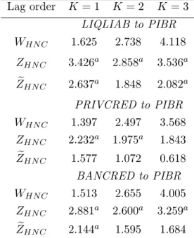
For all the samples considered, we test the causality from …nancial development to
growth and the reverse causality relationship. In each case, we compute three
statis-tics: the average Wald statistic WHN C
N;T , the standardized statistic ZN;THN C based on the
asymptotic moments and the standardized statistic eZN;THN C based on the approximation
of …nite sample moments. In order to assess the sensitivity of our results to the choice
of the common lag-order, we compute all these statistics for one, two and three lags.
The results for the complete sample of 63 developed and developing countries are
reported in tables 2 and 3. When the inference is based on the asymptotic standardized
statistic ZN;THN C, the homogenous non causality (HNC) from …nancial development to
economic growth is generally rejected at a 5% signi…cant level, whatever the variable
used. The only exception is for the PRIVCRED indicator in a model with three lags.
based on the approximation of the moments in a …nite T sample. When the inference
is based on eZN;THN C, the HNC hypothesis from PRIVCRED to PIBR is not rejected for
all lags. The results are ambiguous for the two other indicators. Such results clearly
indicate that the use of the asymptotic Wald distribution in pure time series Granger
causality tests may lead to a fallacious inference in panel with a relatively short time
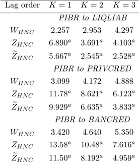
dimension as in our case. These …rst conclusions must be put in prospect compared to
those which one obtains for the causality analysis from economic growth to …nancial
development. In this case (table 3), the HNC hypothesis is strongly rejected and this
conclusion is robust to the choice of the lag-order and the …nancial indicator. Moreover,
the rejection of the null hypothesis is so robust that similar conclusions are obtained
with the asymptotic standardized statistic. The past values of the economic growth
are then useful when one comes to forecast the development of the domestic …nancial
system, in at least one country of the panel.
Insert tables 2 and 3
Our results clearly indicate that in one case (from economic growth to …nancial
development) the non causality hypothesis is strongly and robustly rejected, whereas in
the other case (from …nancial development to economic growth) the same homogeneous
non causality hypothesis is not robustly rejected. The value of the average of individual
Wald statistics is representative of this opposition: for instance, with the PRIVCRED
indicator and K = 1, the value of WN;THN C is slightly superior to 3 when we consider
the in‡uence of growth on …nancial development, whereas the realisation of the same
statistic is only equal to 1:39 when the reverse relationship is considered. The same
tables 11 and 12, in appendix B).
One important issue is to determine if the lack of robustness of the supply-leading
hypothesis is a common characteristic of developed and developing countries. For that,
we consider the same tests for a sub-sample of 35 developing countries (tables 4 and 5)
and a sub-sample of 28 developed countries (tables 6 and 7).
Insert tables 4 and 5
In both cases, the conclusions are similar to those obtained in the complete
sam-ple. As far as the developing countries sample are concerned, the conclusions are even
clearer. We can observe that the HNC hypothesis from …nancial development to
eco-nomic growth is not strongly and robustly rejected when the inference is based on the
…nite sample properties. Similar conclusions are drawn with LIQLIAB and BANCRED
when the asymptotic standardized statistic is used. On the contrary, the causality from
economic growth to …nancial development is largely and robustly accepted, except with
the …rst indicator LIQLIAB. Of course, it seems inappropriate to invoke the
demand-following hypothesis in this context. On the contrary, if there is a causal relationship
from the real side of the economy to the …nancial system in developing countries, it is
perhaps and paradoxically in respect to Patrick’s point of view, a signs of a developing
economy. This causal relationship may reveal an endemic ”fragility” of the
develop-ing countries’…nancial system. Because of the incomplete diversi…cation of risks (due
to incomplete …nancial markets) or a lack of …nancial skills of bankers due to a lack
of training and/or corruption for example, the …nancial system’s condition depends
…nan-cial depth in the short run in less-developed countries. Some recent …nan…nan-cial crises,
like in Argentina, Brazil or South Korea for example, seem to have been the direct
consequence of real factors.
Insert tables 6 and 7
The conclusions for the developed countries are more in favour of the supply-side
hypothesis, even if the results depend on the indicator used and on the lag structure.
With the PRIVCRED indicator, the HNC is not rejected for all lags, whereas the
op-posite conclusion is founded with LIQLIAB. But, it is important to note that the value
of the average Wald statistic for a given indicator is always superior in the developed
countries sample than in the developing countries one. So, it seems that the supply-side
hypothesis is more likely to be accepted in our panel of developed countries than in
the panel of developing countries. The more the countries are developed, the more the
…nancial development is useful in the forecasts of real GDP growth. Finally, as for
the two others samples, the causality from economic growth to …nancial development
is founded to be very robust in this sample. This is conform to the demand-following
hypothesis: this economic growth which generates a demand for …nancial services and
consequently have a positive in‡uence on …nancial deepening.
To sum it up, the lack of robustness of the causal relationship from …nancial
de-velopment to economic growth is conform to the idea that supply-leading hypothesis
is inaccurate for developed economies. Nevertheless, our results do not validate the
Patrick’s hypothesis for the developing countries. We …nd almost the same results when
does not mean that there is no impact of …nancial development on economic growth. In
our opinion, this only shows that the relationship between the two variables is perhaps
too complex to be identi…ed in a short run bivariate Granger causality approach. In a
moral hazard or adverse selection context, the …nancing capacity becomes indeed very
largely dependant of the quality of …nancial governance (Stulz, 2000). The latter is
strongly determined both by the e¢ ciency of legal framework and by its capacity to
guarantee investors’ rights: “In the end, the rights create …nance” (La Porta et al.,
1999). Empirically, La Porta et al. (1997) attempted to assess the contributions of the
legal framework type3, of di¤erent variables measuring the quality of legal framework,
and of various instrumental variables (e.g. growth of GDP, level of GDP) to external
capitalization4. They found that even if the kind of legal framework is not always a
signi…cant variable, the one called “rule of law” is generally very signi…cant.
Identi-cally, Beck et al. (2000) revealed a signi…cant impact of legal framework on growth
and …nancial e¢ ciency5. This empirical studies illustrate the fact that both …nancial
development and economic growth might be tied to a third variable: the quality of
the institutional framework. That is perhaps why we do not …nd any direct observable
Granger causality between the two variables.
There is also a second way to explain this result: the causality from …nancial
de-velopment to economic growth could indeed be a long run relationship. In this case,
the causal relationship must be identi…ed as in Toda and Philips (1993). However,
3
According to them, every legal framework is tied to one of these four historical types: Anglo-Saxon Common Law, French Code Civil, German tradition and Scandinavian tradition.
4
Measured by the ratio: capitalization controlled by external shareholders / GDP.
5
Financial e¢ ciency is an index developed by Demirgürc-Kunt & Levine [1999]. It is equal to the logarithm of the ratio: …nancial transactions / index of banking operations cost.
none generalization in a panel model of the Toda and Phillips approach have been yet
proposed. Such a development is in our work program. So, as far as Granger non
causality tests, there is trade-o¤ between implementing tests on individual time series
with a long-run causality dimension but poor properties due to the short time
dimen-sion, and implementing a panel data test with no long-run dimension but better …nite
sample properties. The only point that we can mention here, is the recent work of
Christopoulos and Tsionas (2004). Using panel unit root and cointegration tests, they
investigate the long run relationship between …nancial depth6 and economic growth
over the 1970-2000 period for 10 developing countries7. One of their conclusions is that
“there is fairly a strong evidence in favor of the hypothesis that long run causality runs
from …nancial development to growth. [...] The empirical evidence also points out to
the direction that there is no short run causality” (p. 72). Our panel Granger non
causality tests con…rm the second part of their results.
5
Conclusion
This paper re-examines the causal relationship between …nancial development and
eco-nomic growth in 63 industrial and developing countries over the 1995 and
1960-2000 periods. We use a new panel test of the Granger non causality hypothesis. The
…ndings can be summarized as follows. First, the Homogenous Non Causality (HNC)
hypothesis from …nancial development to economic growth is very often accepted at 5%
level. We …nd the same result when the panel is split into two subgroups: developed
and developing countries. This suggests that either there is no empirical evidence of
6
In their paper, …nancial depth is the ratio of total bank deposits liabilities to nominal GDP.
7Colombia, Paraguay, Peru, Mexico, Ecuador, Honduras, Kenya, Thailand, Dominican Republic
a causal in‡uence of …nancial depth on economic growth in the short run or that the
causality from …nance to the real side of the economy is too complex relationship to
be identi…ed by a bivariate Granger causality test. Then, our results are then conform
to some conclusions of previous empirical studies (Christopoulos and Tsionas, 2004,
for example). In terms of economic policy recommendations, it implies that …nancial
liberalization could have only delayed positive e¤ect on economic development, or have
an indirect e¤ect on it. That is perhaps why most …nancial liberalization policies which
were implemented in developing countries have been very often unsuccessful in the short
run. Second, the HNC hypothesis is robustly and strongly rejected when we investigate
the causal relationship from economic growth to …nancial development. This result are
conform to Patrick’s demand-following hypothesis when we focus on developed
coun-tries. In that context, economic growth can actively stimulate the demand for …nancial
services. But the reason why this causal relationship exists in developing countries
might be quite di¤erent. It could be a sign of the fragility of …nancial environment
A
Data appendix
All individual …nancial series can be downloaded at the following internet address: http://legacy.csom.umn.edu/WWWPages/FACULTY/RLevine/Index.html. All GDP series can be downloaded at the following internet address:
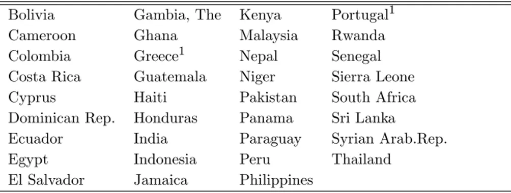
http://datacentre2.chass.utoronto.ca/pwt/alphacountries.html. The classi…cation of countries used in the paper is the following.
Insert tables 8 and 9
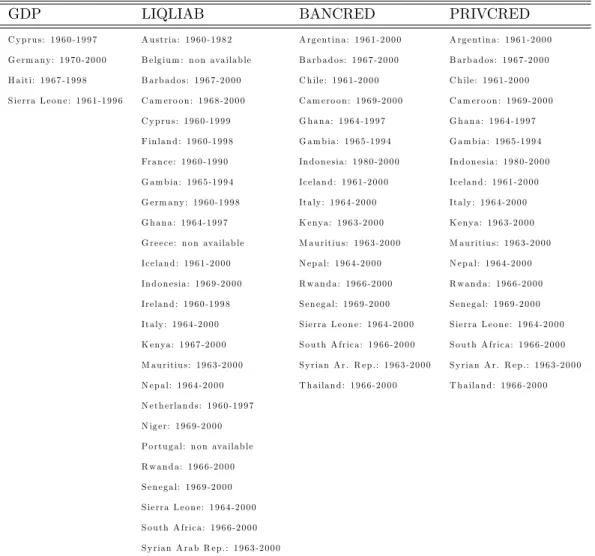
Most individual series starts in 1960 and ends in 2000. However, some of them are incomplete in the sense that they begin later or / and …nish earlier. This implies that panels we use are unbalanced ones. Individual samples for countries which data are incomplete are reported in the table 10.
B
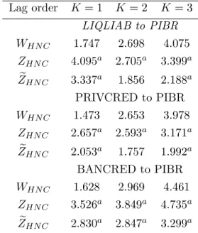
Sensitivity analysis
The two …rst tables 11 and 12, the results obtained with a panel of 63 countries over the period 1960-2000, are reported.
Insert tables 11 and 12
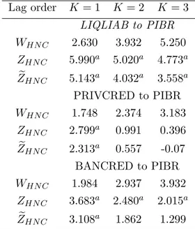
On tables 13 and 14, the results for the sample of 28 countries over the period 1960-2000, are reported.
Insert tables 13 and 14
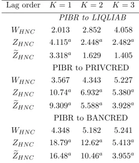
On tables 15 and 16, the results for the sample of 35 developing countries over the period 1960-2000, are reported.
References
[1] Al-Yousif, Y. K., 2002. Financial development and economic growth. Another look at the evidence from developing countries. Review of Financial Economics 11, 131– 150.
[2] Beck, T., Demirguc-Kunt, A., Levine, R. and Maksimovic, V., 2000. Financial structure and economic development: …rm, industry, and country evidence. World Bank working paper 2423, World Bank, Washington, DC.
[3] Calderon, C., Liu, L., 2003. The direction of causality between …nancial develop-ment and economic growth. Journal of Developdevelop-ment Economics 72, 321–334. [4] Christopoulos, D. M., Tsionas, E. G., 2004. Financial development and economic
growth: evidence from panel unit root and cointegration tests. Journal of Devel-opment Economics 73, 55–74.
[5] Demetriades, P.O., Hussein, K.A., 1996. Does …nancial developement cause eco-nomic growth? Time-series evidence from 16 countries. Journal of Development Economics 51, 378–411.
[6] Demirgüc-Kunt, A., Levine, R., 1999. Financial Structures Across Coun-tries:Stylized Facts. Washington, D.C.: World Bank, mimeo.
[7] De Gregorio, J., Guidotti, P.E., 1995. Financial Development and Economic Growth. World Development 23(3), 433–448.
[8] Granger, C.W.J., 1969. Investigating causal relationd by econometric models and cross-spectral methods. Econometrica 37, 424–438.
[9] Greenwood, J. Smith, B.D., 1997. Financial markets in development and the de-velopment of …nancial markets. Journal of Economic Dynamics and Control 21, 145–181.
[10] Hurlin C., 2005, Un Test Simple de l’Hypothèse de Non Causalité dans un Modèle de Panel Hétérogène, Revue Economique, 56(3), 799-809.
[11] Hurlin, C., 2007., Testing for Granger Non Causality in Heterogeneous Panels, Working Paper LEO, Université d’Orléans, 2007-10
[12] Im, K.S., Pesaran, M.H., Shin, Y., 2003. Testing for Unit Roots in Heterogeneous Panels. Journal of Econometrics 115(1), 53–74.
[13] Jung, W.S., 1986. Financial Development and Economic Growth: International Evidence. Economic Development and Cultural Change 34(2), 336–346.
[14] King, R.V, Levine, R., 1993a. Finance and Growth: Schumpeter might be right. Quarterly Journal of Economics 108, august, 717–738.
[15] King, R.V, Levine, R., 1993b. Finance, Entrepreneurship, and Growth: Theory and evidence. Journal of Monetary Economics 32, 513–542.
[16] La Porta, R., Lopez-de Silanes, F., Shleifer, A., Vishny, F., 1997. Legal determi-nants of external …nance. Journal of Finance 52(3), 1131–50.
[17] La Porta, R., Lopez-de Silanes, F., Shleifer, A., 1999. Corporate ownership around the world. Journal of Finance 54(2), 471–517.
[18] Levine, R., Loayza, N., Beck, T., 2000. Financial intermediation and growth: causality and causes. Journal of Monetary Economics 46, 31–77.
[19] Maddala, G.S. Wu, S., 1999. A Comparative Study of Unit Root Tests with Panel Data and a New Simple Test. Oxford Bulletin of Economics and Statistics, special issue, 631–652.
[20] McKinnon, R.I., 1973. Money and Capital in Economic Development. The Brook-ings Institution, Washington DC.
[21] Nair-Reichert, U. Weinhold, D., 2001. Causality tests for cross-countries panels: a look at FDI and economic growth in less developed countries. Oxford Bulletin of Economics and Statistics 63, 153–171.
[22] Patrick, H.T., 1966. Financial Development and Economic Growth in Underdevel-oped Countries. Economic Development and Cultural Change 14, 174–189. [23] Roubini, N., Sala-i-Martin, X., 1995. A growth model of in‡ation, tax evasion, and
…nancial repression. Journal of Monetary Economics 39, 275–301.
[24] Shaw, E.S., 1973. Financial Deepening in Economic Development. Oxford Univer-sity Press, New-York.
[25] Stulz, R., 2000. Does …nancial structure matter for economic growth? a corporate …nance perspective, in: Demirgürç-Kunt, A., Levine R. (Eds.), Financial Structure and Economic Growth, the MIT Press, Cambridge, pp. 143–188.
[26] Swamy, P. A., 1970. E¢ cient inference in a random coe¢ cient regression model. Econometrica 38, 311–323.
[27] Toda, H.Y. Phillips, P.C.B., 1993. Vector AutoRegressions and Causality. Econo-metrica 61, 1367–1393.
[28] Weinhold, D., 1996. Tests de causalité sur données de panel: une application à l’étude de la causalité entre l’investissement et la croissance. Economie et Prévision 126, 163–175.
Table 1: Panel Unit Root Tests V ariable WIP S PM W ZM W PIBR 30:11 (0:00) 901:0 (0:00) 48:82(0:00) BANCRED 20:27 (0:00) 648:8 (0:00z) 32:93(0:00) PRIVCRED 23:24 (0:00) 714:3 (0:00) 37:06(0:00) LIQLIAB 27:17 (0:00) 830:3 (0:00) 45:85(0:00)
Notes: WIP S denotes the standardized IP S statistic based on simulated
approximated moments (Im, Pesaran and Shin, 2003, table 3). PM W
de-notes the Fisher’s test statistic proposed by Maddala and Wu (1999) and on individual ADF p-values. Under H0; PM W has a 2 distribution with
2N of freedom when T tends to in…nity and N is …xed. ZM W is the Choi
(2001) standardized statistic used for large N samples: under H0; ZM W
has a N (0; 1) distribution when T and N tend to in…nity. Corresponding p-values are in parentheses.
Table 2: Causality from Financial Development to Economic Growth. 63 Countries Lag order K = 1 K = 2 K = 3 LIQLIAB to PIBR WHN C 1.625 2.738 4.118 ZHN C 3.426a 2.858a 3.536a e ZHN C 2.637a 1.848 2.082a PRIVCRED to PIBR WHN C 1.397 2.497 3.568 ZHN C 2.232a 1.975a 1.843 e ZHN C 1.577 1.072 0.618 BANCRED to PIBR WHN C 1.513 2.655 4.005 ZHN C 2.881a 2.600a 3.259a e ZHN C 2.144a 1.595 1.684 Notes: aindicates rejection at 5% level.
Table 3: Causality from Economic Growth to Financial Development. 63 Countries Lag order K = 1 K = 2 K = 3 PIBR to LIQLIAB WHN C 2.257 2.953 4.297 ZHN C 6.890a 3.691a 4.103a e ZHN C 5.667a 2.545a 2.528a PIBR to PRIVCRED WHN C 3.099 4.172 4.888 ZHN C 11.78a 8.621a 6.123a e ZHN C 9.929a 6.635a 3.833a PIBR to BANCRED WHN C 3.420 4.640 5.350 ZHN C 13.58a 10.48a 7.616a e ZHN C 11.50a 8.192a 4.959a Notes: aindicates rejection at 5% level.
Table 4: Causality from Financial Development to Economic Growth . 35 Developing Countries Lag order K = 1 K = 2 K = 3 LIQLIAB to PIBR WHN C 1.083 2.113 3.472 ZHN C 0.341 0.325 1.108 e ZHN C 0.022 -0.152 0.312 PRIVCRED to PIBR WHN C 1.217 2.685 4.015 ZHN C 0.908 2.026a 2.452a e ZHN C 0.497 1.219 1.149 BANCRED to PIBR WHN C 1.290 2.614 4.168 ZHN C 1.215 1.818 2.821a e ZHN C 0.764 1.047 1.411 Notes: aindicates rejection at 5% level.
Table 5: Causality from Economic Growth to Financial Development. 35 Developing Countries Lag order K = 1 K = 2 K = 3 PIBR to LIQLIAB WHN C 2.013 2.852 4.058 ZHN C 4.115a 2.448a 2.482a e ZHN C 3.318a 1.629 1.405 PIBR to PRIVCRED WHN C 2.251 3.854 4.754 ZHN C 5.234a 5.486a 4.237a e ZHN C 4.252a 4.073a 2.413a PIBR to BANCRED WHN C 2.242 3.876 4.533 ZHN C 5.197a 5.552a 3.703a e ZHN C 4.219a 4.127a 2.033a Notes: aindicates rejection at 5% level.
Table 6: Causality from Financial Development to Economic Growth. 28 Industrial Countries Lag order K = 1 K = 2 K = 3 LIQLIAB to PIBR WHN C 2.287 3.501 4.907 ZHN C 4.731a 3.901a 4.046a e ZHN C 3.919a 2.937a 2.774a PRIVCRED to PIBR WHN C 1.623 2.263 3.010 ZHN C 2.333a 0.697 0.022 e ZHN C 1.821 0.229 -0.469 BANCRED to PIBR WHN C 1.791 2.705 3.803 ZHN C 2.962a 1.867 1.735 e ZHN C 2.377a 1.228 0.928 Notes: aindicates rejection at 5% level.
Table 7: Causality from Economic Growth to Financial Development. 28 Industrial Countries Lag order K = 1 K = 2 K = 3 PIBR to LIQLIAB WHN C 2.557 3.076 4.590 ZHN C 5.721a 2.795a 3.373a e ZHN C 4.785a 1.994a 2.220a PIBR to PRIVCRED WHN C 4.160 4.569 5.056 ZHN C 11.82a 6.797a 4.443a e ZHN C 10.20a 5.432a 3.141a PIBR to BANCRED WHN C 4.893 5.595 6.371 ZHN C 14.56a 9.513a 7.284a e ZHN C 12.62a 7.749a 5.461a Notes: aindicates rejection at 5% level.
Table 8: High income countries (28)
Argentina Chile Ireland Netherlands United Kingdom
Australia Denmark Israel New Zealand United States
Austria Finland Italy Norway Uruguay
Barbados France Japan Sweden Venezuela
Belgium1 Germany Mauritius Switzerland
Canada Iceland Mexico Trinidad and Tobago 1
N o t in th e liq u id lia b ilit ie s p a n e l d a t a s e t.
Table 9: Low- and middle-income countries (35)
Bolivia Gambia, The Kenya Portugal1
Cameroon Ghana Malaysia Rwanda
Colombia Greece1 Nepal Senegal
Costa Rica Guatemala Niger Sierra Leone
Cyprus Haiti Pakistan South Africa
Dominican Rep. Honduras Panama Sri Lanka
Ecuador India Paraguay Syrian Arab.Rep.
Egypt Indonesia Peru Thailand
El Salvador Jamaica Philippines
Table 10: Samples for incomplete individual series
GDP LIQLIAB BANCRED PRIVCRED
C y p ru s : 1 9 6 0 -1 9 9 7 A u s t ria : 1 9 6 0 -1 9 8 2 A rg e ntin a : 1 9 6 1 -2 0 0 0 A rg e nt in a : 1 9 6 1 -2 0 0 0
G e rm a ny : 1 9 7 0 -2 0 0 0 B e lg iu m : n o n ava ila b le B a rb a d o s : 1 9 6 7 -2 0 0 0 B a rb a d o s : 1 9 6 7 -2 0 0 0
H a iti: 1 9 6 7 -1 9 9 8 B a rb a d o s : 1 9 6 7 -2 0 0 0 C h ile : 1 9 6 1 -2 0 0 0 C h ile : 1 9 6 1 -2 0 0 0
S ie rra L e o n e : 1 9 6 1 -1 9 9 6 C a m e ro o n : 1 9 6 8 -2 0 0 0 C a m e ro o n : 1 9 6 9 -2 0 0 0 C a m e ro o n : 1 9 6 9 -2 0 0 0 C y p ru s : 1 9 6 0 -1 9 9 9 G h a n a : 1 9 6 4 -1 9 9 7 G h a n a : 1 9 6 4 -1 9 9 7 F in la n d : 1 9 6 0 -1 9 9 8 G a m b ia : 1 9 6 5 -1 9 9 4 G a m b ia : 1 9 6 5 -1 9 9 4 Fra n c e : 1 9 6 0 -1 9 9 0 In d o n e s ia : 1 9 8 0 -2 0 0 0 In d o n e s ia : 1 9 8 0 -2 0 0 0 G a m b ia : 1 9 6 5 -1 9 9 4 Ic e la n d : 1 9 6 1 -2 0 0 0 Ic e la n d : 1 9 6 1 -2 0 0 0 G e rm a ny : 1 9 6 0 -1 9 9 8 Ita ly : 1 9 6 4 -2 0 0 0 It a ly : 1 9 6 4 -2 0 0 0 G h a n a : 1 9 6 4 -1 9 9 7 K e nya : 1 9 6 3 -2 0 0 0 K e nya : 1 9 6 3 -2 0 0 0
G re e c e : n o n ava ila b le M a u rit iu s : 1 9 6 3 -2 0 0 0 M a u ritiu s : 1 9 6 3 -2 0 0 0
Ic e la n d : 1 9 6 1 -2 0 0 0 N e p a l: 1 9 6 4 -2 0 0 0 N e p a l: 1 9 6 4 -2 0 0 0
In d o n e s ia : 1 9 6 9 -2 0 0 0 R w a n d a : 1 9 6 6 -2 0 0 0 R w a n d a : 1 9 6 6 -2 0 0 0
Ire la n d : 1 9 6 0 -1 9 9 8 S e n e g a l: 1 9 6 9 -2 0 0 0 S e n e g a l: 1 9 6 9 -2 0 0 0
Ita ly : 1 9 6 4 -2 0 0 0 S ie rra L e o n e : 1 9 6 4 -2 0 0 0 S ie rra L e o n e : 1 9 6 4 -2 0 0 0
K e nya : 1 9 6 7 -2 0 0 0 S o u t h A fric a : 1 9 6 6 -2 0 0 0 S o u t h A fric a : 1 9 6 6 -2 0 0 0
M a u rit iu s : 1 9 6 3 -2 0 0 0 S y ria n A r. R e p .: 1 9 6 3 -2 0 0 0 S y ria n A r. R e p .: 1 9 6 3 -2 0 0 0
N e p a l: 1 9 6 4 -2 0 0 0 T h a ila n d : 1 9 6 6 -2 0 0 0 T h a ila n d : 1 9 6 6 -2 0 0 0 N e t h e rla n d s : 1 9 6 0 -1 9 9 7 N ig e r: 1 9 6 9 -2 0 0 0 P o rt u g a l: n o n ava ila b le R w a n d a : 1 9 6 6 -2 0 0 0 S e n e g a l: 1 9 6 9 -2 0 0 0 S ie rra L e o n e : 1 9 6 4 -2 0 0 0 S o u t h A fric a : 1 9 6 6 -2 0 0 0 S y ria n A ra b R e p .: 1 9 6 3 -2 0 0 0
Table 11: Causality from Financial Development to Economic Growth . 63 Countries, 1960-2000 Lag order K = 1 K = 2 K = 3 LIQLIAB to PIBR WHN C 1.747 2.698 4.075 ZHN C 4.095a 2.705a 3.399a e ZHN C 3.337a 1.856 2.188a PRIVCRED to PIBR WHN C 1.473 2.653 3.978 ZHN C 2.657a 2.593a 3.171a e ZHN C 2.053a 1.757 1.992a BANCRED to PIBR WHN C 1.628 2.969 4.461 ZHN C 3.526a 3.849a 4.735a e ZHN C 2.830a 2.847a 3.299a Notes: aindicates rejection at 5% level.
Table 12: Causality from Economic Growth to Financial Development. 63 Countries, 1960-2000 Lag order K = 1 K = 2 K = 3 PIBR to LIQLIAB WHN C 2.188 3.231 4.829 ZHN C 8.822a 4.768a 5.786a e ZHN C 7.551a 3.636a 4.167a PIBR to PRIVCRED WHN C 3.699 4.336 5.275 ZHN C 15.14a 9.271a 7.373a e ZHN C 13.22a 7.553a 5.503a PIBR to BANCRED WHN C 4.188 5.143 6.340 ZHN C 17.89a 12.47a 10.82a e ZHN C 15.73a 10.39a 8.467a Notes: aindicates rejection at 5% level.
Table 13: Causality from Financial Development to Economic Growth . 28 Countries, 1960-2000 Lag order K = 1 K = 2 K = 3 LIQLIAB to PIBR WHN C 2.630 3.932 5.250 ZHN C 5.990a 5.020a 4.773a e ZHN C 5.143a 4.032a 3.558a PRIVCRED to PIBR WHN C 1.748 2.374 3.183 ZHN C 2.799a 0.991 0.396 e ZHN C 2.313a 0.557 -0.07 BANCRED to PIBR WHN C 1.984 2.937 3.932 ZHN C 3.683a 2.480a 2.015a e ZHN C 3.108a 1.862 1.299 Notes: aindicates rejection at 5% level.
Table 14: Causality from Economic Growth to Financial Development. 28 Countries, 1960-2000 Lag order K = 1 K = 2 K = 3 PIBR to LIQLIAB WHN C 2.907 3.662 5.449 ZHN C 7.007a 4.318a 5.195a e ZHN C 6.040a 3.409a 3.884a PIBR to PRIVCRED WHN C 3.863 4.326 5.334 ZHN C 10.71a 6.156a 5.043a e ZHN C 9.434a 5.082a 3.868a PIBR to BANCRED WHN C 5.070 5.907 7.096 ZHN C 15.22a 10.33a 8.849a e ZHN C 13.49a 8.744a 7.097a Notes: aindicates rejection at 5% level.
Table 15: Causality from Financial Development to Economic Growth . 35 Developing Countries, 1960-2000 Lag order K = 1 K = 2 K = 3 LIQLIAB to PIBR WHN C 1.025 1.688 3.113 ZHN C 0.103 -0.893 0.265 e ZHN C -0.146 -1.138 -0.263 PRIVCRED to PIBR WHN C 1.253 2.876 4.614 ZHN C 1.061 2.593a 3.899a e ZHN C 0.695 1.850 2.705a BANCRED to PIBR WHN C 1.628 2.969 4.884 ZHN C 3.526a 3.849a 4.551a e ZHN C 2.830a 2.847a 3.242a Notes: aindicates rejection at 5% level.
Table 16: Causality from Economic Growth to Financial Development. 35 Developing Countries, 1960-2000 Lag order K = 1 K = 2 K = 3 PIBR to LIQLIAB WHN C 2.013 2.852 4.058 ZHN C 4.115a 2.448a 2.482a e ZHN C 3.318a 1.629 1.405 PIBR to PRIVCRED WHN C 3.567 4.343 5.227 ZHN C 10.74a 6.932a 5.380a e ZHN C 9.309a 5.588a 3.928a PIBR to BANCRED WHN C 4.348 5.182 5.241 ZHN C 18.79a 12.62a 5.413a e ZHN C 16.48a 10.46a 3.955a Notes: aindicates rejection at 5% level.