HAL Id: hal-01895339
https://hal.archives-ouvertes.fr/hal-01895339
Submitted on 15 Oct 2018HAL is a multi-disciplinary open access archive for the deposit and dissemination of sci-entific research documents, whether they are
pub-L’archive ouverte pluridisciplinaire HAL, est destinée au dépôt et à la diffusion de documents scientifiques de niveau recherche, publiés ou non,
an electrical resistivity tomography device
Milia Fares, Géraldine Villain, Stéphanie Bonnet, Sergio Palma-Lopes, Benoit
Thauvin, Mickaël Thiery
To cite this version:
Milia Fares, Géraldine Villain, Stéphanie Bonnet, Sergio Palma-Lopes, Benoit Thauvin, et al.. Deter-mining chloride content profiles in concrete using an electrical resistivity tomography device. Cement and Concrete Composites, Elsevier, 2018, 94, pp. 315-326. �10.1016/j.cemconcomp.2018.08.001�. �hal-01895339�
Determining chloride content profiles in concrete using an
1
Electrical Resistivity Tomography device
2 3
Milia FARES1, Géraldine VILLAIN1, Stéphanie BONNET2, Sérgio PALMA LOPES1, 4
Benoit THAUVIN3, Mickaël THIERY4. 5
6 1
IFSTTAR, Centre de Nantes, Allée des Ponts et Chaussées, CS 5004, 44344 Bouguenais, France
7
[email protected], [email protected], [email protected] 8
2 UBL, Université de Nantes, GeM, Institut de Recherche en Génie civil et Mécanique, 52 rue Michel Ange, BP 9
420, 44 606 Saint-Nazaire, France
10
3 CEREMA DTER Ouest, Département Laboratoire de St-Brieuc, France 12
4
Ministère de la Transition Ecologique et Solidaire, MTES – MCT / DGALN / DMUP
14 [email protected] 15 16 Abstract: 17 18
Chloride penetration in concrete can lead to steel corrosion which is one of the major 19
pathologies affecting reinforced concrete’s durability. The development of methods to 20
investigate chloride penetration is essential to predict and update the service life of the 21
structure. A non-destructive (ND) DC-electrical technique is used in this study: this 22
Electrical Resistivity Tomography (ERT) device is arranged in a Wenner configuration 23
and measures apparent resistivities. Apparent resistivities are then inverted in order to 24
obtain a resistivity profile versus depth. In parallel, a calibration method relating the 25
resistivity to the chloride content for each type of concrete is used to obtain the chloride 26
profile versus depth. This methodology was applied to a chloride diffusion experimental 27
program on two concrete formulations and one mortar. The profiles evaluated by NDT 28
are then compared to those obtained by a destructive method (potentiometric titration). 29
Both types of profile fit relatively well, thus, the presented methodology is validated for 30
determining chloride content profiles by means of a non-destructive ERT device. The 31
evaluation of the uncertainty range of successive processes (measurement, inversion and 32
calibration) underlines the importance on including the uncertainties in the 33
interpretation of the ND profiles in future research. 34
35
Keywords: Resistivity, chloride, NDT, diffusion, concrete durability 36
37
1. Introduction:
38
The deterioration of reinforced concrete structures in marine environment is mainly due to the 39
corrosion of steel induced by the penetration of chloride ions [1]. Chloride ions can penetrate 40
into concrete through multiple mechanisms including diffusion, adsorption, permeation and 41
surface deposit of airborne salts [2-7]. By penetrating into the cover concrete, the chloride 42
ions destroy the passive layer that protects the reinforcing steel bars from corrosion. The 43
corrosion mechanism induces a reduction of the steel surface area and rust production on the 44
bars resulting in an increase of the total volume up to 600% [8, 9]. The consequences then 45
include the decrease of the mechanical resistance of the structure as well as the cracking and 46
the spalling of the concrete. 47
The duration preceding the destruction of the passive layer is defined according to Tuutti [10] 48
as the initiation period which is followed by the propagation period during which the 49
corrosion develops. The work presented in this paper is positioned in the framework of the 50
inspection of concrete structures in marine environment during this initiation period. 51
Determining the chloride concentration at the depth of the steel bars allows evaluating the 52
corrosion risks (studies claim a free chloride threshold varying between 0,07 and 1,16% by 53
weight of binder [11]). Before reaching the critical chloride threshold, the monitoring of the 54
evolution of chloride profile permits the assessment of maintenance needs and repair action 55
scheduling [1, 4, 8]. Moreover, the monitoring of the evolution of the chloride profiles allows 56
the update of the service life prediction models of the structures. 57
Therefore, it is important to determine the chloride concentration profiles and not only to 58
detect the presence of chloride ions or to assess the chloride concentration at only a given 59
depth. This study deals with determining the chloride concentration profiles in cover concrete 60
versus depth using a non-destructive method applied to the concrete surface. 61
Among the few testing techniques used to determine chloride concentration most are 62
destructive, fastidious and time-consuming [12]. One of the main disadvantages of 63
destructives techniques lies in the fact that by destroying the sample, it is not possible to 64
monitor the evolution of the chloride concentration with time at the same position. Hence, the 65
development of fast and reliable non-destructive methods becomes a necessity. 66
With non-destructive methods, the rapidity of the measurement makes it possible to 67
investigate a large surface area of the structure and therefore to detect weak points that need 68
further investigation [13, 14]. In addition, being non-invasive, the methods allow surveying 69
the same spot in the structure and assessing the concrete conditions at several test times. The 70
monitoring parameters provided are valuable to predict the potential evolution of the concrete 71
conditions with time. 72
Amongst non-destructive methods, electromagnetic techniques are particularly sensitive to the 73
resistance (applied voltage divided by transmitted current intensity) of a unit volume of 77
concrete. 78
In concrete, electrical current is carried by the ions present in the pore solution [26]. The 79
resistivity thus depends on the concrete composition (affecting the porosity and tortuosity), on 80
the saturation degree and on the ionic content of the pore solution [20, 27-34]. Concerning the 81
concrete composition, [32] have demonstrated that resistivity increases when the W/C ratio of 82
the studied concrete decreases and therefore when porosity decreases. A similar trend is 83
observed by [35] after measuring concrete specimens with different water to binder ratios. 84
Developed resistivity instruments used on concrete include embedded sensors [36,37] as well 85
as surface applied devices [18].Concerning the saturation degree and the ionic content, 86
although the use of DC-electrical resistivity measurements to assess moisture and ionic 87
contents is fairly common in the fields near-surface geophysics applied to soil science (e.g. 88
[38]), and hydrological or environmental studies (e.g. [39]), approaches are less advanced in 89
the field of concrete durability evaluation. 90
Recent studies [18, 40] have proven the potential of resistivity techniques to monitor water 91
and chloride ingress in concrete by using electrical resistivity measurements. In [18] the 92
authors compare the potential of three electromagnetic (EM) NDT techniques (electrical 93
resistivity tomography (ERT), capacimetry, and ground-penetrating radar) to monitor water 94
and chloride ingress into cover concrete and point out that separating the influences of both 95
parameters (moisture and chloride contents) in non-saturated concrete would imply a more 96
sophisticated and combined EM approach. In [31] the authors focused on evaluating the 97
detection threshold of chlorides in cover concrete by means of an embedded DC-electrical 98
resistivity probe (for monitoring purposes) and based on statistical analysis and quality 99
assessment approaches. Nevertheless, none of these studies are able to quantify the degree of 100
saturation or the chloride content because the calibration phase is missing. In particular, Du 101
Plooy et al. [18] could not decorrelate the effect of the chloride content from the water 102
saturation profile during a sea water imbibition process, on the apparent resistivities measured 103
by the ERT device. 104
For a given cement type, a given concrete mix design, and for a zero chloride concentration, a 105
variation in resistivity most likely indicates a variation of the concrete saturation degree. In 106
the same way, for a given cement type, a given concrete mix design, and for a constant 107
saturation degree equal to 100%, a variation in resistivity most likely indicates a variation of 108
the chloride concentration. 109
It is worth noting that this study deals with chloride diffusion in saturated concrete (S = 110
100%) with the only variant being therefore the chloride content. Although the rate of 111
chloride penetration in non-saturated conditions is more important and is found in various 112
field situations, separating the two parameters is essential at first given that the resistivity is 113
sensitive to both parameters. 114
In this paper, we investigate the use of electrical resistivity tomography (ERT) to obtain a 115
chloride profile concentration using the ERT device developed by [41], by means of one-116
dimension (1D) inversion of raw resistivity data (as opposed to [41] who used a 2D inversion 117
procedure that is somewhat unnecessary for yielding 1D profiles) in addition to material 118
calibration. The article first gives a detailed description of the proposed methodology to 119
obtain chloride content profiles using non-destructive surface measurements. The 120
methodology is validated with an experimental program carried out on three different 121
materials and the results are compared to those obtained by a destructive method. 122
2. Proposed methodology and experimental measurement methods
123
As previous studies [18, 40] did not succeed in determining the chloride profiles by ERT, the 124
innovative methodology described in this section is necessary. 125
2.1 Global methodology to obtain chloride profiles using NDT, including methodology 126
steps 127
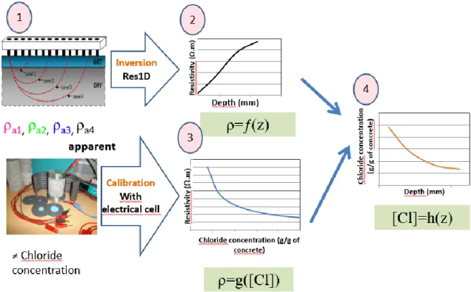
Five main steps can be identified in the process of obtaining a chloride content profile using 128
resistivity measurements (illustrated in Figure 1). 129
The first step is the measurement of a set of apparent resistivities (ρa) on the studied structure
130
using an ERT device (defined in section 2.2.2). Apparent resistivities are the electrical 131
responses of a given material. Each apparent resistivity is obtained by multiplying a measured 132
electrical resistance in Ohms (ratio between the generated potential drop and the 133
corresponding applied current intensity) by a geometric factor (in meters) that accounts for the 134
measurement geometry (see 2.2.2). 135
For a homogeneous and isotropic material, the apparent resistivities theoretically equal the 136
bulk resistivity of the material. In non-homogeneous materials, each apparent resistivity is an 137
obtain a resistivity profile versus depth. The inversion was carried out using the free Res1D 141
software (released for academic use) as will be described in section 2.3. 142
Parallel to this procedure, the third step entails the measurement of the resistivity of several 143
cores of the same concrete saturated with different concentrations of sodium chloride using 144
the calibration resistivity cell (section 2.2.1): this step is to establish the calibration curves 145
corresponding to the resistivity versus the free chloride content. The free chloride content in 146
concrete was determined by the destructive method described in section 2.4. The calibration 147
is, for the time being at least, a necessary tool in order to convert the resistivity profile 148
obtained in step 2 into chloride concentration profile (step 4). The last step deals with 149
transforming the resistivity profile (step 2) to chloride content profile using the calibration 150
curves obtained with step 3. The propagation of uncertainty throughout the different steps 151
listed above has a considerable impact on the final results as will be detailed in section 4.3. 152
To validate the chloride profiles obtained in step 4, these are compared with those obtained by 153
the destructive method described in section 2.4. 154
155
Figure 1 Schematic representation of the methodology used to obtain chloride content profiles in concrete 156
2.2 Resistivity measurement techniques 158
In this section, we present the two techniques, first, the resistivity cell for determining the 159
calibration curves on cores and, second, the ERT device for carrying out apparent resistivity 160
measurements in situ or on slabs at the lab scale. The resistivity cell as well the as the ERT 161
device (also called resistivity probe in [18, 41]) used in this study were developed by Du 162
Plooy et al. [41]. 163
2.2.1 Electrical resistivity cell used for calibration 164
The main use of the resistivity cell is the measurement of the apparent resistivity of small 165
concrete cores (75 mm diameter and 70 mm height) saturated with different chloride contents 166
in order to establish the calibration curve specific to each material. The cell is made of a 167
cylindrical PVC support in which five “ring” electrodes were placed (Figure 2 (a)). The 168
electrodes are made of conductive metallic sponges that are carefully humidified before the 169
test to insure a better contact with the concrete. An electrical current, of intensity I, is injected 170
through two metallic plate electrodes placed on the top and bottom ends of the core 171
respectively as shown in Figure 2 (a). Potential differences ∆Vi are then measured between the
172
various ring pairs in order to assess the homogeneity of the core. The apparent resistivity 𝜌𝑎𝑖
173
for each ring pair is then obtained using (equation 1): 174
𝜌𝑎𝑖 = 𝐺𝑖∆𝑉𝑖
𝐼 (1)
175
where 𝐺𝑖 is a geometric factor equal to 𝐴/𝐿𝑖 (Figure 2) (where A is the area of each electrode
176
plate and Li the distance between the ring electrodes used). Four measurements are performed
177
between two consecutive rings and two measurements are performed between the two 178
extreme rings totalizing therefore six measurements. 179
In this study, having saturated the whole core in the same NaCl solution, we assume each core 180
to be homogeneous. Therefore, regardless of the electrode configuration, all the 𝜌𝑎𝑖 181
theoretically equal the concrete resistivity. The measured apparent resistivities are averaged 182
over all ring electrode pairs and the standard deviation is calculated and is considered as the 183
uncertainty value of the measurements. 184
185
Figure 2 Electrical resistivity cell: the cell used (a) and schematic view of the general principle (b) [43] 186
187
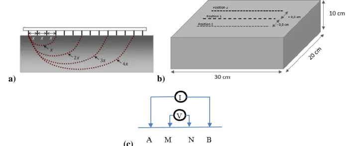
2.2.2 Electrical Resistivity Tomography device 188
The ERT device (Figure 3) can be used in situ on concrete structures. In this study it was 189
implemented on rectangular concrete slabs and used in Wenner configuration (Figure 3 (c)). 190
This device was successfully used to image the penetration of water and different sodium 191
chloride solutions in concrete slabs [40, 41, 43, 44] and was compared to other 192
electromagnetic techniques and destructive methods. It is composed of 14 hollow metallic 193
electrodes filled with wetted sponges. The distance between the centers of the electrodes is 194
equal to 2 cm. The Wenner configuration was chosen due to its high signal-to-noise ratio and 195
high sensitivity to resistivity variation with depth [42]. This electrode configuration implies 196
that the electrodes are aligned and equally spaced and that the current is injected through two 197
outer electrodes and the potential difference is measured between the two inner electrodes. By 198
increasing the spacing between the electrodes, the investigation depth increases [43]. Having 199
14 electrodes, one has access to 4 different electrode spacings and therefore 4 different 200
investigation depths referred to as “levels” as shown by Figure 3 (a). 201
a) b) 202
(c) 203
Figure 3 Schematic representation of the ERT device: (a) penetration depths, (b) device position on the slab, (c) 204
Wenner configuration 205
206
Equation (1) is then applied to obtain the apparent resistivities with the geometric factors 𝐺. 207
For an infinite homogeneous half-space medium, the geometric factor is equal to 𝐺𝑅 = 2𝜋𝑎 208
where 𝑎 is the spacing between the electrodes. However, for a finite medium, boundary 209
conditions need to be taken into account. As explained in [41], the geometric factors in this 210
study are calculated using the COMSOL Multiphysics finite element software and account for 211
both the electrode spacing and the slab geometry. 212
It is worth noting that according to du Plooy [43] the modelled geometric factors are not 213
influenced by the electrode sizes, whether they were modelled using point-electrodes or 4 mm 214
diameter sponge electrodes. 215
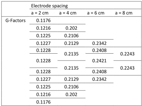
As an example, the geometric factors obtained for the slab studied in the experimental 216
program (section 3.3) are showed in Table 1. 217
As expected, the lowest geometric factors are found for the smallest electrode spacing and for 218
the electrodes positioned near the edges. For more information on the analysis and 219
determination of the geometric factors, the reader can refer to [41,43]. 220
222 Electrode spacing a = 2 cm a = 4 cm a = 6 cm a = 8 cm G-Factors 0.1176 0.1216 0.202 0.1225 0.2106 0.1227 0.2129 0.2342 0.1228 0.2135 0.2408 0.2243 0.1228 0.2421 0.2135 0.2243 0.1228 0.2408 0.1227 0.2129 0.2342 0.1225 0.2106 0.1216 0.202 0.1176
Table 1: Geometric factors computed by FEM for the ERT deviced placed in the central upper face of a 30x20x10cm 223
slab 224
As previously mentioned, for a non-homogeneous material, the obtained apparent resistivities 225
do not directly yield the ‘true’ resistivity distribution of the medium. To obtain the resistivity 226
distribution versus depth in the non-homogeneous, an inversion process is needed (step 2 in 227
our methodology). The inversion process is explained in section 2.3. 228
Three sets of measurements are performed: one in the middle of the slab (Position 1 in Figure 229
3 (b)) and two 5 mm apart from either side of the middle (Position 2 and 3 in Figure 3 (b)). 230
For each set of measurement: the number of electrode combinations and therefore the number 231
of apparent resistivity measured are 11 for Level 1 followed by 8 for Level 2, 5 for Level 3 232
and 2 for Level 4. The different values obtained for the three sets of measurement are 233
averaged per level and four apparent resistivity values are determined, one per investigation 234
level (ρa1, ρa2, ρa3, ρa4). The different values of apparent resistivity obtained per level can be
235
an indicator of the lateral heterogeneity of the slab. This factor is taken into account in this 236
study by the standard deviation of the different apparent resistivity values per level (σ1, σ2, σ3,
237
σ4). Since the volume investigated increases from Level 1 to Level 4, the effect of the vertical
238
heterogeneity on the measurement decreases when the electrode spacing increases. 239
2.3 Inversion process of the measured apparent resistivities 240
The inversion process consists in finding a resistivity profile (in 1D, or resistivity distribution 241
in 2D or 3D) that would yield the same measurements as the actual measurements on the 242
investigated medium [41, 45]. The inversion of the apparent resistivity values of the 4 243
different levels was carried out as stated before using Res1D which is a program based on 244
Levenberg-Marquardt’s algorithm (also known as damped least-squares [46]). Three sets of 245
apparent resistivities were then chosen for the inversion: the mean values (ρa1, ρa2, ρa3, ρa4),
246
the mean values plus the standard deviations (ρa1 +σ1, ρa2 + σ2, ρa3+ σ3, ρa4 + σ4,) and the
247
mean values minus the standard deviations (ρa1 - σ1, ρa2 - σ2, ρa3 - σ3, ρa4 - σ4). The reason for
248
the three sets of inversion is to study the effect of the variability of the apparent measurements 249
(data input) on the inverted resistivity profiles (data output). 250
The material was considered to be composed of 4 ‘homogeneous’ layers (discrete 251
parametrization) with predefined thicknesses estimated with Res1D using the electrodes 252
configuration. The inverse problem consists in obtaining the resistivity values for each layer. 253
The resistivity profile was then estimated by displaying the resistivity at the center of each of 254
the four layers (at 5.1, 16.57, 30.92 and 44.44 mm depth respectively) with horizontal lines 255
corresponding to the thicknesses of the respective layers (equal to 10.2, 12.75, 15.94 and 20 256
mm). 257
It is worth noting that the thicknesses of the layers were determined by estimating the depth of 258
investigation for each electrode separation [47]. This choice for the layer thicknesses may 259
have an effect on the inverted results, i.e. the fitted resistivity of each layer and therefore the 260
obtained resistivity profile. Indeed, it is a long established fact among the geophysics 261
community that “electrical equivalences” may occur between layer models that yield the same 262
apparent resistivities within the data uncertainty level (e.g. [48]). However, other inversion 263
strategies not presented here (including not fixing the layer thicknesses and therefore 264
inverting for both thicknesses and resistivities of layers) did not lead to better fits. 265
In future work, attention should be paid to the development of algorithms using optimized 266
model parameterizations, e.g. a discrete parameterization based on a larger number of layers 267
or a continuous parameterization based realistic resistivity profile shapes. 268
2.4 Destructive method to determine free chloride profiles 269
The adopted reference method is the well-known procedure recommended by the RILEM 270
178-TMC Technical Committee [12, 49]. In order to obtain a profile, the concrete specimens 271
The procedure described below is used to determine the free chloride content from concrete 275
powder [49, 51]. Approximately 5g of concrete powder is taken from each layer and placed in 276
a beaker. To get free chloride, deionised water is added and the mixture is stirred for 3 min. 277
The obtained solution is then filtered into a 250 cm3 volumetric flask. The chloride 278
concentration of the filtered solutions is determined by potentiometric titration with silver 279
nitrate (AgNO3).
280
It is worth noting that the total chloride content in concrete is the sum of the free chlorides in 281
the pore solution and the chlorides that are bound to the cement paste (physically or 282
chemically) [52]. In this research, we study mainly the free chlorides for two reasons: the first 283
is that the corrosion risk of the steel mainly depends on the free chlorides and the second 284
reason is that the electric current in concrete is carried by the ions present in the concrete 285
pores solution [26]. 286
287
3. Experimental program: materials, specimens and measurements
288
procedures
289
The global methodology developed in section 2 was applied on an experimental program on 3 290
types of material. The descriptions of the experimental program as well as the measurement 291
procedures are detailed in the following. 292
3.1 Concrete mix designs and specimens 293
The experimental program was carried out using 2 types of concrete: C1 and C2, and one type 294
of mortar M2. The different components of the materials are represented in Table 2. Concrete 295
C1 is an industrial concrete whereas the other materials were fabricated in the lab under 296
controlled conditions. Concrete C1 was one year old at the time of the test and was kept under 297
ambient temperature conditions in laboratory (T = 20±2°C and RH = 50±7%). C2 and M2 298
were around 8 years old at the time of the test and were conserved alternatively in water or 299
ambient temperature. The three materials were chosen to have a water to cement ratio (W/C) 300
superior to 0.6 to accelerate the penetration of aggressive agents. 301
C1 C2 and M2 Components (kg/m3) Origin C1 (kg/m3) Origin C2 (kg/m3) M2 (kg/m3) Aggregate (11/22) Pont de Pierre,
corneen 760 0 0
Aggregate (6/10) Trégueux, amphibolite 320 Pontreaux, gneiss 785 0 Sand (0/4) Moulin, alluvial 300 Pilier, alluvial 445 649 Sand (0/2) Gouviard, gneiss 560 Pontreaux, gneiss 449 652 Cement C CEM I 52.5 N Saint-Pierre la Cour, Lafarge 305 Saint-Pierre la Cour, Lafarge 341 492
Admixture, AD Sika prise SC2 0.7 0 0
Added water 235 331.9 Effective water W 190 222.9 319.5 W/C 0.623 0.654 0.649 Percentage of cement paste (%) 0,3 0,36 0,51 Dmax [mm] 22 10 5
Table 2 Concrete mix design of concretes C1 and C2 and mortar M2 303
304
The concrete properties are given in Table 3: the values provided are the average values 305
obtained from three experimental results. The open porosity was determined by water 306
saturation under vacuum condition and the apparent diffusion coefficient was determined by 307
chloride migration test in non-steady- state [53]. 308
Material
Open porosity measured by water saturation at 90 days (%) Apparent diffusion coefficient (x10-12 m2/s) [53] Compressive strength at 28 days (MPa) C1 15.9 ± 0.7 21.9 ± 7.6 36.3 ± 0.9 C2 17.5 ± 0.6 55.4 37.1 ± 0.8 M2 26.4 ± 0.5 62.1 34.0 ± 1.0
Table 3 Properties of concretes C1 and C2 and mortar M2 309
310
The experimental program included two main types of experiments: the calibration of the 311
Concerning the specimens, for each material, we dispose of 8 cores used for calibration (with 315
a 75 mm diameter and a 70 mm height). Moreover, we dispose of four slabs 316
(300x220x100 mm): two slabs for C1 (C1-1 and C1-2), one slab for C2 (C2-1) and one slab 317
for M2 (M2-1) used for chloride diffusion. 318
3.2 Calibration: Core conditioning and measurement procedure with EM cell (Step 3 in 319
Section 2.1) 320
For calibration purpose, the resistivity has to be measured at different chloride contents. For 321
each 3 concretes, the 8 cores (75x70 mm) were initially dried in an oven at 65°C until mass 322
stability according to the criteria defined by [54] (i.e. the relative difference of 2 weighing 323
results with a 24h gap must be under 0.05%). We assume actually that the studied concrete 324
materials are fully hydrated and hydrates like ettringite remain stable below 70°C [55]. The 8 325
cores were afterwards saturated using a vacuum-chamber with solutions having 4 different 326
sodium chloride concentrations (0, 15, 35 and 90 g/L) in addition to 4 g/L NaOH to avoid 327
leaching as recommended by the French standards [56-57] (2 cores per concentration). The 328
cores were then stored for 5 months in a solution (regularly renewed) with the same sodium 329
chloride concentration as the one they were saturated with. 330
For each concentration, two cores of each concrete were conditioned and tested with the 331
resistivity cell in order to obtain the calibration curves. After the first set of 6 measurements is 332
performed, the core is rotated and a second set of 6 measurements is performed. Having 12 333
resistivity measurements per core (at different heights of the core), the total number of 334
resistivity measurements is 24 per material per concentration. The average of the 24 335
measurements as well as the standard-deviation are computed. 336
At the end of the non-destructive testing, the “real” free chloride concentrations were 337
determined for one of the two cores at 4 different heights (approximately 5, 20, 40 and 60 338
mm), using the destructive protocol detailed in section 2.4. To get the concentration at 5 mm, 339
the core was ground in several steps from 0 to 10 mm, perpendicular to the top face of the 340
specimen using the grinding instrument. To get the value at 20 mm, 40 mm and 60 mm, the 341
core was ground respectively from 10 to 30 mm, from 30 to 50 mm, and from 50 to 70 mm. 342
The average of the concentrations obtained at the four different heights as well as the standard 343
deviation were then calculated and are presented in the calibration curves (Figure 5) in section 344
4.1. 345
3.3 Chloride diffusion monitoring: Slab conditioning and non-destructive testing 346
procedure with ERT device 347
The chloride diffusion experimental program was carried out under saturated conditions 348
which entails that the main mode of transport of chloride ions is due to the concentration 349
difference between the external solution and the interstitial water. In preparation for the 350
diffusion experimental program, the 4 slabs (C1-1 and C1-2, C2-1, M2-1) were saturated in a 351
vacuum chamber with chloride free tap water. An epoxy resin was then applied on the lateral 352
faces of the slab to ensure a unidirectional transfer. 353
The slabs were then placed in individual closed boxes. The bottom face was placed in 354
regularly renewed solutions containing 165 g/l NaCl and 4 g/l NaOH up to 1 cm, at initial test 355
time. The upper face was covered with a wet cloth to prevent evaporation (see Figure 4). 356
At each test time, each slab was removed from solution and carefully wiped with a wet cloth 357
before apparent resistivity measurement with the ERT device. The measurements were carried 358
out at the 3 positions indicated at section 2.2.2 and on both sides. Right after the 359
measurements, the slab was placed again in the solution again in the same way as for the 360
initial test time. 361
Using this same protocol, the apparent resistivity measurements were regularly performed for 362
a period of 18 weeks for C1-1, 40 weeks for C1-2 and 12 weeks for each of C2-1 and M2-1. 363
364
Figure 4 Scheme of the chloride diffusion protocol 365
366
4. Results and discussions
analysis of uncertainty sources is led. Finally, the chloride content profiles extracted from 370
ERT measurements are compared to reference destructive profiles at final test times. 371
372
4.1 Calibration results: Chloride concentration as a function of resistivity (Step 3) 373
As explained before, the calibration curves are needed to convert the resistivity profile 374
obtained in step 2 into chloride concentration profile (step 4). It is shown in this paragraph 375
how the calibration curves are obtained for each concrete. 376
The resistivity versus chloride concentration calibration curves for the three materials are 377
presented in Figure 5. The average resistivity (standard-deviation given by vertical error bars) 378
measured in homogeneous cores is function of the average of the concentrations (standard 379
deviation as horizontal error bars) obtained by the reference chloride titration. For all the 380
cases, the chloride content was found to be homogeneous throughout the core with the 381
maximal variation coefficient attaining 6%. 382
In order to compare the materials, in Figure 5 (a) we represent the concretes C1 and C2, and 383
in Figure 5 (b) we represent the concrete C2 and mortar M2. The experimental results show a 384
fast decrease of the resistivity at low concentrations and a slow decrease at higher 385
concentrations, similarly to the results of [31], [32] and [58]. Therefore, the results were 386
modeled using an exponential curve with regression coefficients superior to 0.9. Three curves 387
were obtained by fitting the average experimental points (blue solid line) and the average plus 388
and minus the vertical and horizontal standard-deviation (pink and green dashed lines). 389
As mentioned before, the resistivity and the diffusivity of concrete are strongly related since 390
they are both dependent on the tortuosity and porosity of the material. When the diffusivity is 391
higher, the current is lead more easily through the concrete and the resistivity is therefore 392
lower. Comparing the two concretes, the resistivity of the saturated concrete C1 (initially 393
around 50 Ω.m) is superior to that of the saturated C2 (initially around 30 Ω.m), the latter 394
being superior to that of M2 (initially around 20 Ω.m). The results are in agreement with the 395
values obtained for the apparent coefficient of diffusion (Table 3) where that of C1 (21.7x10 -396
12
m2/s) is inferior to that of C2 (55.4x10⁻¹² m2/s), the latter being inferior to that of M2 397
(62.1x10⁻¹² m2/s). This general trend also applies for the samples with chloride. 398
399
Figure 5 Calibration curves relating resistivity versus free chloride concentrations 400
- (a) concretes C1 and C2 - (b) concrete C2 and mortar M2 401
402
4.2 Monitoring resistivity versus time during chloride diffusion process (Step 1) 403
We present herein the chloride diffusion monitoring results. The apparent resistivities of the 404
concretes measured during the experimental program are inverted. Then the true resistivity 405
profiles are translated into chloride concentrations using the calibration curves. 406
4.2.2 Variation of resistivity with time during chloride diffusion 407
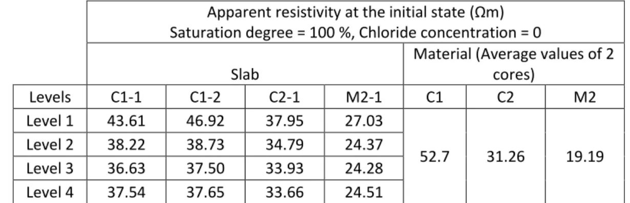
4.2.2.1 Initial state 408
The apparent resistivity measured for each Level (Level 1 to 4) versus time of diffusion is 409
presented in Figure . 410
As indicated before, the slabs were saturated in vacuum in order to obtain a homogeneous 411
saturated slab (saturation = 100%, chloride concentration = 0 g/l). Therefore, at the initial 412
state, the resistivity results at the different levels (or different investigated depths) were 413
expected to be equal. However, the apparent resistivity at Level 1 is superior to the resistivity 414
of the other Levels indicating an initial property gradient in the concrete (Table 4). This initial 415
gradient can either be due to a porosity difference (due to carbonation, framework effects, 416
shrinkage, …) or to an ionic difference in the material (leaching). 417
valued to be more likely due to a possible leaching whose influence on resistivity 421
measurement is underlined by [20] and not to carbonation or water saturation degree 422
difference. In the future, we plan to control the basicity of the solution in which the concrete 423
is stored in order to avoid any risk of lixiviation problem. In addition, compared to the initial 424
state of the cores used for calibration (Table 4), the resistivity values of the slabs of C1 were 425
expected to be higher, and those of the slabs of C2 and M2 were expected to be lower. The 426
difference between the resistivity values almost certainly lies in the material heterogeneity. 427
This difficulty will be a challenge for in-situ measurements given that the contrast between 428
the samples will be even higher than in the case of laboratory conditions. 429
430
Apparent resistivity at the initial state (Ωm) Saturation degree = 100 %, Chloride concentration = 0
Slab
Material (Average values of 2 cores) Levels C1-1 C1-2 C2-1 M2-1 C1 C2 M2 Level 1 43.61 46.92 37.95 27.03 52.7 31.26 19.19 Level 2 38.22 38.73 34.79 24.37 Level 3 36.63 37.50 33.93 24.28 Level 4 37.54 37.65 33.66 24.51
Table 4 Initial state of the slabs : apparent resisitivty values for Levels 1 to 4 431
432
4.2.2.2 Evolution of apparent resistivity with time 433
For the 4 slabs, the trend of the curves are similar: a decrease of the apparent resistivity values 434
for the 4 levels is noticed due to the penetration of chloride in the concrete. For concrete C1, 435
we chose to prolong the diffusion test for the slab C1-2 up to 40 weeks compared to 18 weeks 436
of test time in the case of slab C1-1. The apparent resistivity values of the four levels continue 437
to mildly decrease after 18 weeks. The standard-deviation (of the three series of 438
measurements) is the highest for Level 1 and decreases from Level 1 to Level 4. Given that 439
the measurement for each Level integrates a certain volume of the slab which increases from 440
Level 1 to Level 4, the resistivity values at Level 4 are less influenced by the local variation in 441
the material. 442
443
444
Figure 6 Evolution of apparent resistivity versus time during a chloride diffusion test for Level 1 to 4 for: slab C1-1 445
(a), C1-2 (b), C2-1 (c) and mortar M2-1 (d) 446
447
Within few days of exposure to chloride , the apparent resistivity values for a given date is 448
increasing from Level 1 to Level 4 which implies a lower resistivity on the surface and a 449
higher resistivity in the core. This is in agreement with the expected direction of chloride ions: 450
from the surface to the core. Therefore, the results indicate a high chloride concentration on 451
the surface and a lower concentration in the core which is in agreement with the physical law 452
of chloride diffusion. 453
The raw results displayed offer a good indicator of the chlorides penetration in the concrete 454
structure, the apparent resistivity can indicate an increase or a decrease of the chloride 457
concentration for a stable saturation degree. 458
However, for a higher accuracy, it would be very useful to obtain not merely the trend of the 459
concentration, but the exact distribution of the chloride concentration in concrete. The next 460
section deals with the sources of uncertainty encountered in the process of obtaining the 461
chloride concentration profile. 462
4.3 Apparent resistivity inversion and sources of uncertainty on the chloride profiles 463
(Step 2 and 4) 464
As detailed in section 2.1, different steps are required to obtain chloride profile from surface 465
resistivity measurements. The steps include mainly an inversion and a calibration process. 466
The variability of the raw data, the material difference between the calibration cores and the 467
diffusion slabs are all sources of uncertainty that will affect the final results. Taking them into 468
account is crucially important and in the next section, a first attempt is presented. 469
The study of the propagation of the uncertainty throughout the different steps of the method is 470
presented solely for concrete C2 as an example. The same analysis was applied to C1 and M2, 471
and the final result will be presented for the 3 materials. 472
4.3.1 Consequences of raw data variability on the inversion results 473
As was elaborated in section 3.3, three sets of raw data were chosen for inversion taking into 474
account the standard deviation. So, the resistivity ρ correspond to the inversion result of the 475
average apparent resistivity ρa and the resistivities, noted ρ- and ρ+ , correspond respectively
476
to the inversion results of ρa – σ and ρa + σ. As an example, the three sets of inversion after
477
0.9 week, 3 weeks, and 11 weeks of concrete C2 are displayed in Figure 7 (a). Three 478
resistivity profiles for each date are obtained: a mean profile ρ (solid line), a maximal profile 479
ρ+ (dotted lines) and a minimal profile ρ- (dashed lines). We remind the reader that the 480
inversion was carried out using a discrete parameterization and horizontal error bars represent 481
the layers thickness. The horizontal bars are represented solely for the inversion of the mean 482
resistivity after 3 weeks of chloride diffusion for visual purposes. 483
To visualize the effect of the resistivity profiles variability on chloride profiles, in Figure 7 (b) 484
we display the three sets of chloride profiles at 11 weeks of diffusion obtained using the three 485
sets of resistivity profiles and the mean curve of calibration (Figure 5 (b)). However, the 486
calibration curves present as well a maximal and minimal variation range that needs to be 487
taken into account. 488
489
Figure 7 Consequences of raw data variability for concrete C2 on the profiles: (a) resistivity profile after 0.9 week, 3 490
and 11 weeks (b) chloride profile after 11 weeks 491
492
4.3.2 Consequences of calibration curve variability on the inversion results 493
The mean resistivity profile obtained after 11 weeks of diffusion (purple solid line in Figure 7 494
(a)) is converted to three chloride profiles (Figure 8 (a) maximal in pink, mean in blue and 495
minimal in green) using the three calibration curves (Figure 5 (b)). The same procedure was 496
applied for the minimal resistivity profile « ρ- » (Figure 8 (b)) and maximal resistivity profile 497
« ρ+ » (Figure 8(c)). Finally, 9 profiles are obtained. In order to assess and show the range of 498
uncertainty, three of the 9 chloride profiles were selected (Figure 9 (c)): the mean profile 499
(solid blue line), the maximal profile (pink dashed line, noted Cl max ρ-) and the minimal 500
profile (dotted green line, noted Cl min ρ+). The drawback is that this choice maximizes the 501
possible variation range of the uncertainty. 502
For the two other materials, the same procedure was applied thus the mean resistivity profile ρ 503
is shown and the variation range between “Cl max ρ-” and “Cl min ρ+”. 504
505
506
Figure 8 Concrete C2 after 11 weeks of diffusion: Minimal, mean, maximal profiles for the inversions of ρ (a), ρ- (b) 507
et ρ+ (c) 508
509
4.4 Comparing chloride profiles obtained by resistivity to those obtained by destructive 510
method 511
The procedure explained in the previous sections has been applied to the three materials: C1, 512
C2 and M2. In addition, for each slab, a destructive chloride profile was obtained using a core 513
(70 cm diameter) from the slab. In Figure 9, the chloride profiles obtained by resistivity are 514
illustrated in three colors (green, blue and pink) and the one obtained by potentiometric 515
titration in black. The vertical error bars for the destructive methods are based on a recent 516
study by Bonnet et. al [59] where the vertical standard deviation for total chloride content is 517
approximately equal to 6% (calculated from 42 measurements). Unfortunately, no studies are 518
found about the sources of uncertainties for the free chloride profile measurements in concrete 519
by destructive method. However, as explained in [59], the protocol for obtaining the total and 520
free chloride profiles are similar. 521
522
523
Figure 9 Comparing chloride profiles obtained by resistivity and those obtained by destructive method for : Slabs C1-524
1 (a), C1-2 (b), C2 -1 (c) and M2-1 (d) 525
526
In general, and considering the horizontal error bars, the destructive profiles lie in the range of 527
the non-destructive profiles. The few differences that can be found between the profiles are 528
attributed to the several sources of uncertainty stated before. More specifically, two main 529
sources can be underlined: 530
2) At the initial state (concrete fully saturated and without chloride), a significant 534
difference was found between the resistivity of the slabs used for the diffusion test and 535
the cores used for the calibration (Table 4). Since the curves displayed in Figure 9 536
were obtained using those calibration curves, a significant difference between the ND 537
results and the D results is expected. 538
539
The diffusion of chloride for concrete C1 lasted for 18 weeks for slab C1-1 (solid line in 540
Figure 10) and for 40 weeks for slab C1-2 (dashed lines in Figure 10). The comparison of the 541
chloride profiles obtained by means of both resistivity and destructive method at the end of 542
the experimental program is presented in Figure 10. 543
The increase of the chloride concentration from 18 weeks (C1-1) to 40 weeks (C1-2) is 544
observed for both the ND and the D profiles. In addition, between the depths of 20 and 36 545
mm, the ND and the D profiles are almost merged. 546
The D profile of C1-1 is superior to that of C1-2 between the depths of 0 and 10.6 mm. This is 547
certainly due to the material difference between both slabs. As stated earlier, the material 548
heterogeneity effect is more pronounced on the surface of the slabs. 549
550
Figure 10 Evolution of chloride profiles for concrete C1 after 18 weeks (slab C1-1) and 40 weeks of chloride diffusion 551 (slab C1-2) 552 553 5 Conclusion 554
In this article, we have presented a methodology that allows obtaining chloride concentration 555
profiles from surface resistivity measurements. The process implies the use of an inversion 556
process to obtain resistivity profiles and a calibration curve to obtain chloride concentration 557
profiles. The methodology was successfully applied to three types of material (two concretes 558
and one mortar). The profiles obtained were compared to those obtained by a destructive 559
method. The non-destructive results were represented by three profiles for each measurement: 560
a mean/intermediate, a maximal and a minimal profile. The three profiles took into 561
consideration the propagation of uncertainty throughout the proposed methodology. In 562
general, the destructive profile was located between the gaps of the three profiles. The highest 563
sources of uncertainty underlined were first the material difference between the samples used 564
for calibration (cores) and those used for the diffusion tests (slabs), and second the automatic 565
inversion process that only allows a discrete parametrization of the modelled medium. 566
To overcome the uncertainty from the inversion process, several solutions can be studied such 567
as the implementation of a continuous parametrization inversion and/or the increase of the 568
number of available data. However, overcoming the uncertainty coming from the material 569
differences is trickier because as stated before, the material difference at on-site 570
measurements is more important than that of laboratory samples. In this case, increasing 571
information about the material (by increasing and varying non-destructive techniques) can 572
aim to assess the difference between the measured samples and those used for calibration. 573
Therefore, the difference can be implemented in the calibration curves and taken in 574
consideration when transforming resistivity values to chloride concentrations. 575
The comparison of two chloride concentration profiles for the same concrete after two 576
different diffusion times highlights the ability of the methodology to monitor the evolution of 577
chloride penetration. In the near future, the study of the evolution of the chloride 578
concentration profiles by means of resistivity can aim to determine durability indicators using 579
chloride penetration models. 580
581
Acknowledgments 582
The authors would like to thank Région Pays de la Loire and IFSTTAR for financial support 583
of the PhD thesis, IFSTTAR and CEREMA for financing the research project ORSI-APOS, 584
Véronique Bouteiller and Jean-Luc Geffard (IFSTTAR), Ronan Queguiner and the technical 585
team from CEREMA Site of Saint Brieuc, for their contribution in the experimental 586
Bibliography 589
[1] V. Baroghel-Bouny, Concrete design for structures with predefined service life durability 590
control with respect to reinforcement corrosion and alkali–silica reaction state-of-the-art and 591
guide for the implementation of a performance-type and predictive approach based upon 592
durability indicators, English version of Documents Scientifiques et Techniques de l’AFGC 593
(Civil Engineering French Association) (2004) 252. 594
[2] L. Pang, Q. Li, Service life prediction of RC structures in marine environment using long 595
term chloride ingress data: Comparison between exposure trials and real structure surveys, 596
Construction and Building Materials 113 (2016) 979–987. 597
[3] W. Chalee, C. Jaturapitakkul, P. Chindaprasirt, Predicting the chloride penetration of fly 598
ash concrete in seawater, Marine Structures 22 (2009) 341–353. 599
[4] I. Othmen, S. Bonnet, F. Schoefs, Investigation of different analysis methods for chloride 600
profiles within a real structure in a marine environment, Ocean Engineering, Volume 157, pp 601
96-107. 602
[5] Hilsdorf, H., Kropp, J., 2004. Performance Criteria for Concrete Durability, CRC Press, 603
2004. 604
[6] A.B. Fraj, S. Bonnet, A. Khelidj, New approach for coupled chloride/moisture transport in 605
non-saturated concrete with and without slag, Construction and Building Materials 35 (2012) 606
761-771. 607
[7] A. Da Costa, M. Fenaux, J. Fernández, E. Sánchez, A. Moragues, Modelling of chloride 608
penetration into non-saturated concrete: Case study application for real marine offshore 609
structures, Construction and Building Materials 43 (2013) 217–224. 610
[8] L. Bertolini, B. Elsener, P. Pedeferri, E. Redaelli, R. Polder, Corrosion of steel in 611
concrete: Prevention, Diagnosis, Repair, 2nd Edition, WILEY-VCH, Weinheim, Germany, 612
2013. 613
[9] A. Neville, Chloride attack of reinforced concrete: an overview, Materials and Structures 614
28 (1995) 63-70. 615
[10] K. Tuutti, Corrosion of Steel in Concrete, Swedish foundation for concrete Research, 616
Stockholm, 1982. 617
[11] U. Angst, B. Elsener, C.K. Larsen, & Ø. Vennesland, Critical chloride content in 618
reinforced concrete—a review. Cement and concrete research 39(12) (2009) 1122-1138. 619
[12] R.T. 178-TMC, Analysis of total chloride content in conrete, Materials and Structures 35 620
(2002 (a)) 583-585. 621
[13] D. Breysse ed., Non-destructive Assessment of Concrete Structures: Reliability and 622
Limits of Single and Combined Techniques: State-of-the-art Report of the RILEM Technical 623
Committee 207-INR, Springer, Netherlands, 2012. 624
[14] J.G. Webster, H. Eren, Measurement, Instrumentation, and Sensors Handbook, Second 625
Edition:Spatial, Mechanical, Thermal, and Radiation Measurement., CRC Press,2014. 626
[15] G.E. Monfore, The electrical resistivity of concrete., Journal of PCA (1968) 35-48. 627
[16] A. Robert, Dielectric permittivity of concrete between 50 Mhz and 1 Ghz and GPR 628
measurements for building materials evaluation, Journal of Applied Geophysics 40(1-3) 629
(1998) 89-94. 630
[17] D.A. Whiting, M.A. Nagi, Electrical resistivity of concrete – a literature review, Portland 631
Cemente Association, Skokie (Illinois),2003. 632
[18] R. du Plooy, G. Villain, S. Palma Lopes, A. Ihamouten, X. Dérobert, B. Thauvin, 633
Electromagnetic non-destructive evaluation techniques for the monitoring of water and 634
chloride ingress into concrete: a comparative study, Materials and structures 48 (2015) 369-635
386. 636
[19] R.B. Polder, W.H.A. Peelen, Characterisation of chloride transport and reinforcement 637
corrosion in concrete under cyclic wetting and drying by electrical resistivity, Cement and 638
Concrete Composites 24(5) (Octobre 2002) 427-435. 639
[20] R. Spragg, S. Jones, Y. Bu, Y. Lu, D. Bentz, K. Snyder, J. Weiss, Leaching of 640
conductive species: Implications to measurements of electrical resistivity., Cement and 641
Concrete Composites 79 (May 2017) 94-105. 642
[21] Y. Bu, J. Weiss, The influence of alkali content on the electrical resistivity and transport 643
[22] M. Fares, Y. Fargier, G. Villain, X. Dérobert, S. Palma Lopes, Determining the 646
permittivity profile inside reinforced concrete using capacitive probes, NDT&E international 647
79 (2016) 150-161. 648
[23] G. Klysz, J.P. Balayssac, Determination of volumetric water content of concrete using 649
ground-penetrating radar, Cement and concrete research 37(8) (2007) 1164-1171. 650
[24] X. Dérobert, J. Iaquinta, G. Klysz, J.P. Balayssac, Use of capacitive and GPR techniques 651
for non-destructive evaluation of cover concrete, NDT&E International. 41(1) (2008) 44-52. 652
[25] G. Villain, V. Garnier, M. Sbartaï, X. Dérobert, J-P. Balayssac, Development of a 653
calibration methodology to improve the on-site non-destructive evaluation of concrete 654
durability indicators, Materials and Structures, 2018, 51:40 available on line 655
https://doi.org/10.1617/s11527-018-1165-4 656
[26] R.B. Polder, Test methods for on site measurement of resistivity of concrete -- a RILEM 657
TC-154 technical recommendation, Construction and Building Materials 15(2-3) (2001) 125-658
131. 659
[27] C. Andrade, A. R., Concrete mixture design based on electrical resistivity, Second 660
International Conference on Sustainable Construction Materials and Technologies, Ancona, 661
Italy, 2010, pp. 28-30. 662
[28] H.W. Whittington, J. McCarter, M.C. Forde, The conduction of electricity through 663
concrete, Magazine of Concrete Research 33(114) (1981) 48-60. 664
[29] B.P. Hughes, A.K.O. Soleit , R.W. Brierley New technique for determining the electrical 665
resistivity of concrete, Magazine of Concrete Research 37(133) (1985) 243 –248. 666
[30] W. Elkey, E.J. Sellevold, S. Vegvesen, Electrical resistivity of concrete, Publication No. 667
80 (1995). 668
[31] M. Saleem, M. Shameem, S.E. Hussain, M. Maslehuddin, Effect of moisture, chloride 669
and sulphate contamination on the electrical resistivity of Portland cement concrete, 670
Construction and Building Materials 10 (3) (1996) 209-214. 671
[32] Z.M. Sbartaï, S. Laurens, J. Rhazi, J.P. Balayssac, G. Arliguie, Using radar direct wave 672
for concrete condition assessment: Correlation with electrical resistivity., Journal of Applied 673
Geophysics 62(4) (2007) 361-374. 674
[33] J.F. Lataste, G. Villain, J.P. Balayssac. Chapter 4. Electrical Methods, IN Non-675
destructive Testing and Evaluation of Civil Engineering Structures, BALAYSSAC J-P., 676
GARNIER V. (Eds). Elsevier Press Ltd, Amsterdam, English Version (2017) 356p. ISBN 677
978-1-78548-229-8 https://doi.org/10.1016/B978-1-78548-229-8.50004-2 678
[34] S. Bonnet, J.P. Balayssac, Combination of the Wenner resistivimeter and Torrent 679
Permeameter methods for assessing carbonation depth and saturation level of concrete, 680
Construction and Building Materials, 188 (2018), pp. 1149-1165. 681
[35] A. Lübeck, A.L.G. Gastaldini, D.S. Barin, H.C. Siqueira, Compressive strength and 682
electrical properties of concrete with white Portland cement and blast-furnace slag, Cement 683
and Concrete Composites 34(3) (2012) 392–399. 684
[36] W.J. McCarter, T.M. Chrisp, A. Butler, P.A.M. Basheer, Near surface sensors for 685
condition monitoring of cover-zone concrete, Construction and Building Materials15(2-3) 686
(2001) 115-124. 687
[37] R. Bässler, J. Mietz, M. Raupach, O. Klinghoffer, Corrosion monitoring sensors 688
fordurability assessment of reinforced concrete structures, Materials week, Munich, Germany, 689
September 25th-28th, 2000 690
[38] O. Banton, M.A. Cimon, M.K. Seguin, Mapping field-scale physical properties of soil 691
with electrical resistivity, Soil Science Society of America Journal 61(4) (1997) 1010-10. 692
[39] M.H. Loke, J.E. Chambers, D.F. Rucker, O. Kuras, P.B. Wilkinson, Recent 693
developments in the direct-current geoelectrical imaging method, Journal of Applied 694
Geophysics 95 (2013) 135–156. 695
[40] Y. Lecieux, F. Schoefs, S. Bonnet, T. Lecieux, S.P. Lopes, Quantification and 696
uncertainty analysis of a structural monitoring device: detection of chloride in concrete using 697
DC electrical resistivity measurement, Nondestructive Testing and Evaluation 30(3) (2015) 698
216-232. 699
[41] R. du Plooy, S. Palma Lopes, G. Villain, X. Dérobert, Development of a multi-ring 700
resistivity cell and multi-electrode resistivity probe for investigation of cover concrete 701
[43] R. du Plooy, The development and combination of electromagnetic non-destructive 705
evaluation techniques for the assessment of cover concrete condition prior to corrosion, PhD- 706
Université de Nantes, Ifsttar Nantes, 2013. 707
[44] G. Villain, A. Ihamouten, R. du Plooy, S. Palma Lopes, X. Dérobert, Use of 708
electromagnetic non-destructive techniques for monitoring water and chloride ingress into 709
concrete, Near Surface Geophysics 13(3) (2015) 299-309. 710
[45] W. Menke, Geophysical Data Analysis: Discrete Inverse Theory, Academic press 1989. 711
[46] M. Fares, Evaluation de gradients de teneur en eau et en chlorures par méthodes 712
électromagnétiques non-destructives, PhD, Ecole Centrale de Nantes, Ifsttar, Nantes, 2015. 713
[47] R.D. Barker, Depth of investigation of collinear symmetrical four-electrode arrays. 714
Geophysics 54(8) (1989) 1031-1037. 715
[48] D.S. Parasnis, Principles of applied geophysics. Fourth edition, Chapman & Hall (1986) 716
422 p. 717
[49] R.T. 178-TMC, Analysis of water soluble chloride content in concrete, 718
Recommendation, Materials and Structures 35 (2002 (b)) 586-588. 719
[50] O. Vennesland, M.-A. Climent, C. Andrade, Recommendation of RILEM TC 178-TMC : 720
Testing and modelling chloride penetration in concrete. Methods for obtaining dust samples 721
by means of grinding concrete in order to determine the chloride concentration profile, Mater 722
Struct : RILEM Technical Committee (2012). 723
[51] T. Chaussadent, G. Arliguie, AFREM test procedures concerning chlorides in concrete: 724
extraction and titration methods, Materials and structures 32(3) (1999) 230-234. 725
[52] V. Baroghel-Bouny, X. Wang, M. Thiery, M. Saillio, F. Barberon, Prediction of chloride 726
binding isotherms of cementitious materials by analytical model or numerical inverse 727
analysis, Cement and Concrete Research 42(9) (2012) 1207-1224. 728
[53] N.B. 492, Nordest Method : Chloride migration coefficient from non-steady-state 729
migration experiments, NORDTEST, Espoo, Finland (1999). 730
[54] AFPC-AFREM, Méthodes recommandées pour la mesure des grandeurs associées à la 731
durabilité, Journées techniques AFPC-AFREM sur la durabilité des bétons, Toulouse–France, 732
1997, 283p. 733
[55] Zhou, Q., Glasser, F. P.,Thermal Stability and Decomposition Mechanisms of Ettringite 734
at <120°C. Cement and Concrete Research, 2001, Vol. 31(9), pp.1333-1339. 735
[56] XP P 18-461, Concrete — Chloride migration of hardened concrete in steady state, 736
French standards, AFNOR (2012). 737
[57] XP P 18-462, Concrete — Chloride migration of hardened concrete in non steady state, 738
French standards, AFNOR (2012). 739
[58] F. Hunkeler, The resistivity of pore water solution- a decisive parameter of rebar 740
corrosion and repair methods, Construction and Building Materials 10 (5) (1996) 381-389. 741
[59] S. Bonnet, F. Schoefs, M. Salta, Sources of uncertainties for total chloride profile 742
measurements in concrete: quantization and impact on probability assessment of corrosion 743
initiation, European Journal of Environmental and Civil Engineering (2017). 744
http://dx.doi.org/10.1080/15732479.2017.1377737 745
![Figure 2 Electrical resistivity cell: the cell used (a) and schematic view of the general principle (b) [43]](https://thumb-eu.123doks.com/thumbv2/123doknet/7763975.255603/8.892.194.683.107.293/figure-electrical-resistivity-cell-cell-schematic-general-principle.webp)