3D coding tools final report

(1)

HAL Id: hal-00935604

https://hal.archives-ouvertes.fr/hal-00935604

Submitted on 23 Jan 2014

HAL is a multi-disciplinary open access

archive for the deposit and dissemination of

sci-entific research documents, whether they are

pub-lished or not. The documents may come from

L’archive ouverte pluridisciplinaire HAL, est

destinée au dépôt et à la diffusion de documents

scientifiques de niveau recherche, publiés ou non,

émanant des établissements d’enseignement et de

3D coding tools final report

Vincent Ricordel, Vincent Jantet, Josselin Gautier, Christine Guillemot,

Laurent Guillo, Emilie Bosc, Fabien Racapé, Luce Morin, Muriel Pressigout,

Marco Cagnazzo, et al.

To cite this version:

Vincent Ricordel, Vincent Jantet, Josselin Gautier, Christine Guillemot, Laurent Guillo, et al.. 3D

coding tools final report. 2013, pp.89. �hal-00935604�

(2)

Projet PERSEE

« Schémas Perceptuels et Codage vidéo 2D et 3D »

n◦ _{ANR-09-BLAN-0170}

Livrable D4.3 31/07/2013

3D coding tools final report

Vincent RICORDEL IRCYNN

Vincent JANTET IRISA

Josselin GAUTIER IRISA

Christine GUILLEMOT IRISA

Laurent GUILLO IRISA

Olivier LE MEUR IRISA

Emilie BOSC IETR, IRCYNN

Fabien RACAPE IETR, IRISA

Luce MORIN IETR

Muriel PRESSIGOUT IETR

Marco CAGNAZZO LTCI

Giuseppe VALENZISE LTCI

(3)

Contents 2

Introduction

In this document we describe the latest contributions to the PERSEE project related to 3D video compression. Several perceptually-oriented appoaches have been proposed to encode depth information. Several of these algorithms have been integrated with the new 3D-HEVC 3D video codec which is being developped in the ISO/ITU JVT joint standardization group.

(6)

Edge based Depth Map Compression for 3D Coding 5

1 Edge based Depth Map Compression for 3D Coding

1.1 Introduction

At the coding stage along the 3DTV framework, the depth map compression meth-ods have recently gain interest in the video coding community. The transmission of geometry joined to the texture information is necessary to Depth Based Image Ren-dering (DIBR) for interactive multi-view display on 3DTVs. The geometry provided by the depth of the acquired scene will allow the generation of new virtual viewpoints adapted to the end-user’s display requirements: additional viewpoints inside or outside of the range of transmitted views to offer more views and then extend the range of stereoscopic vision on auto-stereoscopic displays for example.

It is indeed essential to efficiently encode and reconstruct a depth map in a way that preserves the distance properties of objects within each other because this will be precisely used for later view synthesis. In contrast the depth map smoothly varying surface leads to very predictable pixel values along the spatial dimension that might not need to be perfectly reconstructed if they don’t affect the rendering.

A depth map is basically representing different depths of objects in the scene and more exactly different distances to object surfaces. These surfaces are delimited by the object borders. A distortion into the object depth might result in a local deformation of the rendered object, but a distortion at borders between the object and its background depths might lead to worse artefacts: mixed foreground/background object textures.

In this section we will present an efficient depth map compression introducing lossless edge coding as an alternative to 3DVC depth map coding methods approximating piecewise linear functions whose coefficients need to be encoded.

1.2 A Lossless Edge based Depth Map Coding Method

Depth maps have two main features that must be preserved but can also be relied on for efficient compression. The first one is the sharpness of edges, located at the border between object depths. Distortions on edges during the encoding step would cause highly visible degradations on the synthesized views, that may require depth map post-processing. The second one comes from the general smooth surface properties of objects whose depth is measured.

While Merkle et al. first proposed that smooth regions could be approximated by piecewise-linear functions separated by straight lines, we indeed assume that these smooth surfaces could be entirely reconstructed by interpolating the luminance values from their boundaries. Then the coefficients of the piecewise-linear functions would not be transmitted but instead the pixel values on both side of the edges.

To this end, we can observe that depth maps share similarity to cartoon-images. Mainberger et al. [33] proposed a dedicated cartoon-image encoder, that - in low bitrate conditions - beats the JPEG-2000 standard. After a Canny edge detection, the edge locations are encoded with a lossless bi-level encoder, and the adjacent edge pixel values are lossy quantized and subsampled. At the decoding stage, a homogeneous

(7)

diffusion or an interpolation are used to retrieve the inside unknown areas from lossy decoded edges. Indeed, the demonstrated performances -while beating state of the art codecs- reach the limit of 30dB.

We revisited this edge-based compression method by proposing improvements to fit the high quality, low bitrate, and specific requirements of depth maps. Finally, we increase the diffusion-based depth map encoding performance, which might be generalized to all kinds of images.

In the next sections the encoding process is described. Then the decoding, diffusion and interpolation methods are explained. Results, performances and comparison with state-of-the-art methods based on a traditional objective metric are then given in the next section, before subjective experiments draw more meaningful results on the effectiveness of our proposal.

EDGE DETECTION JBIG CODING EDGE INTENSITY EXTRACTION EDGE INTENSITY CODING ALONG PATH ARITHMETIC CODING FRAME+SEED EXTRACTION Payload Edge Location (JBIG) Frame Edge Intensity Seeds JBIG

DECODING EDGE INTENSITY REPOSITION-NING

HOMOGENEOUS DIFFUSION

Fixed directional priority

Figure 1: Diagram of the proposed depth map compression method.

1.2.1 Encoding

The encoding is a 5-step process: first is the detection of edges, then encoding of the edge location and finally encoding of the edge, border and seed pixel values, as illustrated by Figure 1.

Edge detection Different operators exist to extract the contour of an image. An optimal edge detector should provide:

• a good detection: the algorithm should find as much real edges as possible. • a good localization: the edges should be marked as edges as close as possible to

the real edges.

• a good robustness: as much as possible, the detector should be insensitive to noise.

(8)

In our context of depth map edge coding, several requirements are added. The quality of reconstruction by diffusion should be maximized, while minimizing the number of edges to encode. To avoid diffusion from bad positioned edges causing “leakages”, the localization of contours should be quasi-perfect. The detection of contours should be good but avoiding an over-detection. Up to a certain limit, weak contours (i.e. with a low gradient) might be useless for the reconstruction and might unnecessarily increase the edge coding cost. Also, noisily detected pixels should be avoided for the same reason.

The Marr-Hildreth edge detector combined with Canny-like hysteresis thresholding is used in [33], but suffers from errors of localization at curved edges. The widely used Canny edge detector has also been benchmarked. It relies on a 5x5 gradient prefiltering to cope with noise before local maxima edge detection. But this prefiltering step also makes this detector vulnerable to contour localization errors, as illustrated in Figure 2(c), where inexact selection of adjacent edge pixels leads to improper diffusion. In contrast Sobel has the advantage of an accurate contour localization -as shown in Figure 2(d)- at the cost of a noisy, edge detection. To cope with these over-detected edges, contours c shorter than a certain value (c < 14) are excluded. Pixels with a bi-dimensional gradient amplitude larger than a threshold λ are extracted. Used with sharp depth maps, this gives well-localized contours.

Encoding the contour location As in [33], a bi-level edge image containing the exact location of previously detected edges is first encoded using the JBIG (Joint Bi-level

Image Experts Group) standard. This is a context-based arithmetic encoder enabling

lossless compression of bi-level images. We use the JBIG-Kit, a free C implementation of the JBIG encoder and decoder. The progressive mode is disabled to reduce the required bitrate.

Encoding the contour values Once the edge pixel locations have been encoded, the pixel luminance values have also to be losslessly encoded following our initial requirements. The authors in [33] proposed to store the pixel values on both sides of the edge, instead of the pixel values lying on the edge itself. Indeed, for blurry contours, this might be valuable to interpolate the inner part of the edge and code the luminance values on both sides. However, with sharp depth maps, the pixel values lying directly on an edge, as illustrated in Figure 2(b), alternate between one side or another from this edge and couldn’t be interpolated correctly.

With the Sobel edge detection not thinned to a single edge pixel, we ensure retaining at least one pixel value from each side of the frontier edge as shown in Figure 2(d).

We keep the idea of storing the pixel values by their order of occurrence along the edge to minimize signal entropy. A path with fixed directional priorities (E, S, W, N, NE, SE, SW and NW) is used. As the intrinsic properties of pixels along an edge or “isophote” are their small luminance variation, then we propose to compute the differential values of edge pixels in a Differential Pulse Code Modulation (DPCM) way. From this optimized path encoding method, the stream of DPCM values is then encoded with an arithmetic coder.

(9)

(a) (b)

(c) (d) (e)

Figure 2:(a) A “Breakdancer” depth map, (b) the encoded and decoded Sobel edge and seed pixels (red selection on (a)), (c) a zoom (blue selection) on Canny edges, (d) the selection of corresponding pixel adjacent to Canny edges (c) as in [33], with an intruder edge pixel (orange-framed) that will lead to bad diffusion, (e) the proposed Sobel selection of edge pixel values, exactly located from both side of the frontier edge.

(10)

Additionally to these edges we also encode two kinds of information. The pixel values from the image border are stored to initiate the diffusion-based filling from borders. Inspired by the work of [4] on “dithering” for finding optimal data for interpolation, we propose to sparsely deploy, at regular intervals, some seeds of original depth pixels as shown in Figure 2(b) (The interval s = 10 in practice) While having low overhead, we discovered that this helps accurate reconstruction by initializing and accelerating the diffusion in large missing areas.

Thus, these extra border and seed pixels are coded in DPCM and added to the differential edge values. The resulting file is thus composed of the payload of the JBIG data and of the arithmetic encoded bitstream of the DPCM border, edge and seed pixel values. A typical PCM payload and its subsequent DPCM payload (from a depth map encoding of the “breakdancers” sequence) are illustrated in figure 3.

Frame border

Edge

Seeds

PCM DPCM

Figure 3: Illustration of the payload of the encoded pixels intensity values (“break-dancers” depth map). The PCM (left) pixel intensity and the DPCM (right) residuals are displayed in raster scan order.

It can be seen on the PCM values (3 left) that the pixels vary very smoothly along the frame border: the frame border pixel entropy is very low after DPCM on upper part of 3 right. Interestingly , the upper frame border is black while the lower is bright: it comes from the scene configuration: the upper part is the farther part, the background whole, and lower part of the scene is the ground closer to the camera.

The original pixel values of the edge pixels coded with a walk along the edge appear more cluttered: edges pixels contribute the most to the global entropy of the image. The edges are found and coded in a raster -scan order on the whole image: even if the edges have low-varying values along their edges, once an edge is terminated, the iterative process follow the encoding from the next vertex whose values can be very

(11)

different. Each jump to the next edge can be illustrated by the higher or lower residual error than the middle gray value in 3 right.

Finally the seeds values appear regular: their luminance is encoded in a raster scan order so the highest residual pixels come from a jump from seeds on background to foreground and reversely.

1.2.2 Decoding, diffusion vs interpolation

A lossless decoding of the border, edges and seeds is performed. Then two methods are proposed and evaluated to reconstruct the depth map surfaces: a lossy diffusion or an interpolation from the decoded edge pixels. Finally, a quadtree approach is proposed to place the seeds.

Decoding contour location and pixel values Once the edge positions from JBIG payload are decoded, the edge pixel values are decoded and positioned following the same order in which they were encoded: the path along contour location respecting directional priorities. The border and seed values are also re-positioned following a predefined location.

Reconstructing the Missing Values by Diffusion We now have a sparse depth map containing only the edge, border and seed pixel values. A homogeneous diffusion-based inpainting approach is used to interpolate the missing data. This method is the simplest of the partial differential equations (PDEs) diffusion method, and has the advantage of low computational complexity. It directly stems from the heat equation:

(

It=0= eI δI δt = ∆I

where eI is the decoded edge image before diffusion that will constitute the Dirich-let boundaries of the equation. The diffused data then satisfies the Laplace equation ∆I = 0. The diffusion process is run in a hierarchical manner, each diffusion step being in addition helped with seeds and appropriate initialization. These three improvements have been introduced in the classical diffusion approach to limit the number of itera-tions required to converge, hence to speed up the entire process.

diffusion A Gaussian pyramid is built from eI. The diffusion process is first performed on a lower level of the pyramid and the diffused values are then propagated to a higher level (3 levels are used and show good performances). The propagation of the blurred version of the diffused pixel values from a lower level to an upper one helps to initialize the diffusion in unknown areas.

Middle range initialization On the highest level, instead of starting from unknown values of eI set at 0, we propose to initialize unknown values to the half of the possible range: 128 for an 8 bit depth map. This facilitates and speeds up the process of diffusion by limiting the number of required iterations to converge.

(12)

Seeding As explained in section 1.2.1, some seeds are chosen from a regular pattern both to accelerate the diffusion process and to provide accurate initialized values in large unknown areas. Indeed, this definitely achieves a fast and accurate diffusion -with a gain of 10 dB- for a quasi-exact reconstruction of the depth map.

Reconstructing the Missing Values by Interpolation A bi-linear interpolation is also tested to render the missing values between border, edges and seeds. A linear interpolation in both directions from the border, edge and seed pixels is simply realized. It is equivalent to a two-table lookup with linear interpolation in both horizontal and vertical directions.

This approach is more simpler than the diffusion one and gives better results: no iterative process of diffusion are required up to an asymptotic point. This will be assessed in the section 1.3.

1.2.3 An Extension by a Quadtree Approach

Another approach has been finally proposed to add flexibility to the coding of seeds. Instead of placing the seeds on a regular pattern, the seeds are positioned on each vertex of blocks obtained from a quadtree decomposition. The original depth map is recursively divided into four equal-sized square blocks based on the presence of edges within the block. If an edge is present within a given block, this block is subdivided into smaller blocks, up to the limit of the smaller size of block.

Because the edge positions are transmitted and the smaller size of block is fixed and known at the decoder side, no quadtree decomposition needs to be conveyed: only the border, edge, and seed -positioned according to the quadtree- values are transmitted in addition to the pixel location.

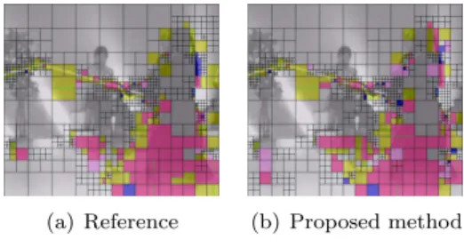
A quadtree decomposition of a “breakdancers” depth map is illustrated in 4(a). The quadtree is well decomposed into smaller blocks along the edges, while big blocks remain in the large smooth areas. However, the interpolation in these areas might be poor because only four seeds at vertices will help the interpolation (except at frame border). Small variation of depth surfaces not extracted by edge detector will not be reproduced on large areas, while they would be partially reproduced with seeds placed on a regular pattern. This will be assessed in the next section. The hypothetical advantage to use seeds placed according to a quadtree rather than on a regular interval is illustrated on Figure 4(b), to compare with 2(b). The seeds are more dense in the neighbourhood of detected edges which might lead to a better interpolation and reconstruction of the small surfaces.

1.3 Results based on objective quality evaluation

The performances of the proposed compression method and its extensions are first evaluated on an objective quality metric ground. An original resolution depth map from a MVD sequence “Breakdancers” from [?] is used. It was accurately estimated through a color segmentation algorithm. The original good quality of the depth map

(13)

(a) (b)

Figure 4: Ilustration of the quadtree decomposition on the criterion of edge presence. (a): Quadtree decomposition blocks are illustrated in white. The minimum size of block is 8x8. (b) A zoom on 2(a) with the seeds positioned according to the quadtree.

will enable a precise evaluation of the impact on texture synthesis reconstruction of the depth distortions.

1.3.1 Depth map objective quality evaluation

The reconstruction quality of our PDE-diffusion-based method is investigated and compared with the JPEG-2000 and HEVC-HM-4.1 Intra compressed versions. First, to visually illustrate the difference of quality reconstruction on edges, the three methods are compared at equal Peak-Signal-to-Noise-Ratio (PSNR),(45 dB, JPEG-2000 with a Quality factor Q=25, HEVC-Q=40).

A zoom on the head of a character presenting initially sharp edges highlights the difference of edge quality depending on the compression type (Figure 5). While at high PSNR, the JPEG-2000 (a) and HEVC (b) versions of the depth map tend to blur the edges. This is commonly referred to as ringing artifacts. It appears with JPEG-2000 because of the lossy quantization following wavelet transformation. It might appear with HEVC because of deblocking filter limitation. Then both JPEG-2000 and HEVC cannot efficiently reconstitute the smooth gradient on uniform areas while preserving the edges. In contrast, our proposed approach stores the exact edges and diffuses regions between these edges, resulting in a smooth gradient restitution on slanted surfaces and non-distorted edges.

Thus we evaluate the global depth-map rate-distortion performances of the three previous encoding methods plus the interpolation and the interpolation-plus-quadtree methods. Figure 6 shows that the diffusion approach outperforms JPEG-2000 except in very low or high bitrate conditions, while being under HEVC. No dedicated adjustment

(14)

(a) (b) (c) (d)

(e) (f) (g) (h)

Figure 5:Upper row: zoom on the head of a dancer on original View #3 (V3) depth map (a) highlights -by comparison at equal depth map PSNR (45dB) referenced to (a)-the ringing artifact on JPEG-2000 (b) and (a)-the blur effect with HEVC (c). Our method (d) based on exact edges and homogeneous diffusion prevents this effect (contrast has been increased on depth maps for distortion visibility). Lower row: zoom on corresponding synthesized view V4 without (e) or with JPEG-2000 (f) and HEVC (g) compressions and our diffusion-based method (h).

was performed in our method, only the threshold λ was varied to adjust its bitrate (an interval of 10 pixels between seeds was chosen for the tests).

The interpolation approach with the same regular pattern of seeds gives substantial improvements in terms of depth map PSNR (with the original depth map as refer-ence). An average gain of 4dB in term of PSNR is obtained in practice between the interpolated-decoded depth map and the diffused-decoded depth map.

With the quadtree approach, the supposed advantage of reduced seed number on the bitrate is counterbalance by the decrease of depth map PSNR quality. For different minimum sizes of quadtree blocks, 8 and 32 pixels, the average fall of quality is of 6dB and 7.5dB on average respectively. The maximum size of quadtree blocks was 512 pixels and might also have been limited to a small size. As proposed before, it is precisely on these large uniform areas that the loss of PSNR quality is important. But have these falls repercursions on the objective visual quality of the synthesized - and then displayed - view? This will be presented in the next section.

1.4 View synthesis quality evaluation

The impact of depth compression methods on rendering is measured by calculating the PSNR of a synthesized view (from a pair of uncompressed textures and compressed depth maps), with respect to an original synthesized view (from a pair of uncompressed textures and depth maps). The corresponding synthesized view from two original

(15)

Edge based Depth Map Compression for 3D Coding 14 0 0.1 0.2 0.3 0.4 40 50 60 Bitrate (bpp) Depth map PSNR (dB) HEVC Intra Interpolation, Seed10 Interpolation, QT8 Interpolation, QT32 Diffusion, Seed10 JPEG-2000

Figure 6: Rate-Distortion performance of the V3 first “breakdancers” depth map with

different quality factors of JPEG-2000 and HEVC and different Sobel detec-tion thresholds λ for the three proposed methods. The proposed methods differ in the interpolation from decoded edges and seeds: diffusion or bi-linear interpolation from regular seeds and bi-linear interpolation from quadtree-placed seeds. 0 0.1 0.2 0.3 0.4 35 40 45 50 Bitrate (bpp) Sy n thesized View PSNR (dB) HEVC Intra Interpolation, Seed10 Interpolation, QT8 Interpolation, QT32 Diffusion, Seed10 JPEG-2000

Figure 7: Rate-Distortion performance of synthesized V4 with the bitrate of V3 depth

map, for different quality factors of JPEG2000 and HEVC, and different Sobel detection thresholds λ for the three proposed methods.

(16)

depth maps is then the reference. VSRS 3.0 [32] is used for view interpolation from this 2-view dataset.

The R-D synthesis performance, illustrated in Figure 7, justifies the edge-coding approach over wavelet based encoders: undistorted edges permit an accurate and ef-ficient view coding and rendering. The PSNR quality of synthesized view is better than JPEG-2000 with the edge-based method with both diffusion or interpolation fill-ing from regular seeds. The interpolation method even beats the HEVC intra coded method for 0.1 to 0.2 bpp. However, the PSNR measure shows its limitation of ob-jective evaluation on perceived quality. Our method does not always outperform in term of rate-distorsion the existing methods (Figures 6, 7), but still can improve the perceived quality of the synthesized view, especially around critical edges (see Figure 5).

The non-linearity of the depth map and synthesized view PSNR quality deserves some explanation. The rate-distorsion PSNR curves are all monotonic but a drop appears with diffusion-based and especially with interpolation-based solutions when the bitrate is reducing under 0.12-0.14 bpp. This can not be explained by the constant cost of seeds along a regular pattern that could become not negligible at low bitrate. The quadtree solution -which effectively reduced the cost of seeds and then the total cost of the methods- still introduces this non-linearity.

This fall might be due to detected edges non-connected anymore. When reducing the bitrate and then the edge detection threshold, the edges around object become non-connected or their edge pixels values along the edge are not well preserved. In those cases with our walk-along-edge technique, when a hole around an edge is encountered, a new vertex non-correlated with the preceding edge pixel has to be transmitted. When this happens over the whole image, the total quality of depth map reconstruction is affected because entire surfaces become poorly interpolated. A solution could be to reconnect the edge pixels at decoding side before interpolating their values along the edges and then between the edges.

1.5 Subjective Results

Subjective assessment of the influence and impact of compressed depth maps on 3D view synthesis have been conducted in the IVC lab of IRRCyN in Nantes. The ex-periments were in line with the MPEG on-going activities on 3D video coding and then relied on similar test conditions and view rendering techniques and the same se-quences as input tested data. These were realized within the PERSEE project context and involved different depth coding methods of four french labs.

The idea was to observe, test and measure the influence of the proposed depth compression method on the perceived visual artefacts of rendered views and then on the consequent perceived visual quality by observers.

(17)

1.5.1 Experimental contents

The first experiment presented below involves the rendering of multiple spatially-translated but temporally-fixed intermediate frames from the same two adjacent views obtained from uncompressed textures and compressed depth images. An intermediate rendering from a pair of frames was processed, then another shifted in space render-ing from the same pair was processed and so on. The resultrender-ing shifted intermediate frames were then concatenated into a single monoscopic video displayed on a mono-scopic screen. This leads to a video where the viewpoint is changing over time while the acquired time doesn’t evolve: a bullet-time effect video.

Depth Map Coding Methods Two state-of-the-art simulcast and one multiview-plus-depth video coding methods are selected for the benchmark: H.264/MPEG-4 AVC, HEVC and 3DVC respectively. The depth coding method is also compared to the recent JPEG-2000 still image coding standard which is based on wavelet-transform and is then supposed to efficiently encode the 8-bits uniform area while limiting the ringing artefacts. The selected method from our previous work was based on interpolation and quadtree seed distribution with a quadtree block minimum size of 32 pixels. This choice was made before the objective quality comparison with previous interpolation methods presented in 1.4. This method was originally selected according to a bitrate criterion to compete with the state-of-the-art 3DVC technique. Finally, filtered and edge-filtered versions of the original depth map are tested for extensive comparisons. Preselection of Coded Depth Map Versions According to the Perceived Synthesized Quality Because the objective quality scores -with their associated bitrate- of depth maps could not give a good opinion on the range of subjective quality of the synthesized views, three experts first pre-selected different qualities of coded depth maps according to three classes of perceived quality of synthesis. This to ensure that the rank were given in roughly the same range of quality. Then the quality of synthesized views could be compared between each other into a dedicated class and evaluated by an observer. Competing with 3D-HTM The main issue when we want to compare a method to another one is how to do that fairly. This issue arises with the comparison of our depth map coding technique to the depth coding method embedded into the 3DVC video standard.

First, while our method does not involve any temporal prediction, it seems fair to compare the rate of the depth map coding technique to the distortion in view synthesis, expressed on a single frame instead of on the whole video. The intra mode of H.264 and HEVC are then used for the single frame comparison. The bitrate of the single Intra coded depth image is then used, while the distortions are evaluated on the resulting rendered temporally-shifted video.

Second, while our method uses in input only a single depth map, the 3DVC depth map coding uses a set of different inter-component prediction techniques to efficiently encode jointly the texture and the depth data (see sections ?? and ??), such as the inter-prediction Mode 3 and 4, but also the View Synthesis Prediction.

(18)

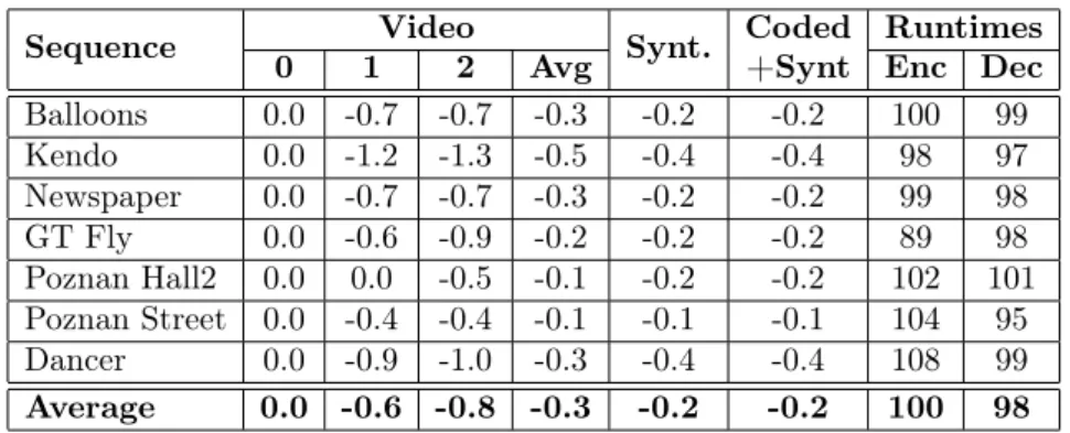
View Synthesis Method The view synthesis method is the same as used by MPEG: the View Synthesis Rendering Software (VSRS). The same software version as cur-rently used for normalization of MPEG 3D-HTM is retained, and the same rendering is used: view interpolation from two adjacent views. Two modes of interpolation are used, either with view blending or without.

The view synthesis is run with a pair of non-compressed texture images and the corresponding pair of compressed depth maps coded with one of the depth coding methods. Then, the impact of the depth map coding is isolated and can be measured independent of texture coding.

Resulting bullet-time video stimuli All the tested methods are compared at three levels of quality of the resulting synthesized view, predefined by a video quality expert. For each depth map coding the blending mode of VSRS is either activated or deacti-vated. Thus, for each method, 3 levels x 2 blending modes are tested, so 6 bullet-time video stimuli were displayed, evaluated and annotated by the viewer.

Between each frame, the intermediate view was shifted1_/

50from the left toward the

right view. When the extreme intermediate right view before the original right view was synthesized, the inverse camera movement was done. Then, 50 resulting frames shifted toward the right plus 50 frames in inverse movement were displayed successively. This allows the viewer to clearly identify the potential artefacts appearing in a moving video -as it will be the case in practice- while the pair of depth maps is the same over time.

Test material Six videos as proposed by MPEG have been retained. Two Class-A Full HD video and four Class-C 1024x768 pixels resolution videos were used.

Sequence Encoded views Displayed views Undo Dancer 1-9 (1 +1_/ 50∗(9−1)−2) → (9 −1/50∗(9−1)−2) GT Fly 1-9 (1 +1_/ 50∗(9−1)−2) → (9 −1/50∗(9−1)−2) Kendo 1-5 (1 +1_/ 50∗(5−1)−2) → (5 −1/50∗(5−1)−2) Balloons 1-5 (1 +1_/ 50∗(5−1)−2) → (5 −1/50∗(5−1)−2) Newspaper 2-6 (1 +1_/ 50∗(5−1)−2) → (5 −1/50∗(5−1)−2) Book Arrival 6-10 (1 +1_/ 50∗(5−1)−2) → (5 −1/50∗(5−1)−2)

Table 1: Selected multi-view video sequences with their respective encoded and dis-played views.

1.5.2 Viewing conditions

The assessment of the quality of the synthesized view was realized on a 2D conven-tional LCD display (Panasonic BT-3DL2550) in a controlled environment (following the recommendations ITU-R BT500-11). For the HD sequences, the observation dis-tance was of 3H (ratio between height of the screen (310mm) and observation disdis-tance (93cm)).

(19)

1.5.3 Participants

27 subjects with normal or corrected-to-normal vision participated in the experiment. The experiment was split into two sessions. Each subject evaluated all the video stimuli.

1.5.4 Test protocol

The subjective assessment was conducted with the Absolute Category Rating with Hidden Reference (ACR-HR) methodology, as set forth in ITU-T recommendation P.910. The test sequences were presented one at a time and rated independently on a category scale. Among the displayed stimuli, a hidden reference was included to prevent the assessment values from being affected by differences in the video content used for assessment. The assessment results obtained by the ACR method are “normal-ized” by using the following formula to calculate the difference in scores between the assessment video and reference video, expressed as DMOS (Differential Mean Opinion Scores):

DMOS = {assessment video score} − {reference video score} + 5

with the quality of the reference video judged to be from “1: Bad” to “5: Excellent” by the subject between each video presentation.

1.5.5 Results: DMOS

The average DMOS of the 27 observers for the “Balloons” and “Book Arrival” bullet-time video synthesized sequences are illustrated in Figures 8. Additional results for the rest of MPEG sequences of 3DVC corpus are presented in Annex ??. Different trends can be observed for the set and for each video sequence. These will be presented before the limitations and perspectives be discussed.

Globally speaking, the evolution of DMOS appears similar between the versions of VSRS rendering with or without blending, and this whatever the sequences.

Also, the 3DVC Intra coding of depth maps generally performs best among the low quality class of video. However, the 3DVC intra coded methods sometimes also present by far the lower subjective quality (Balloons and Kendo not blended). This raises the question of the best trade-off between perceived quality and bitrate requirements.

The compressions of the five methods selected in the middle quality class gives glob-ally a subjective score which is inside the confidence interval: the five methods manage to compress effectively the sequence in a relatively low range of bitrate without affect-ing the perceived visual quality (between 0.025 and 0.04 bpp for class C videos). These two observations are important because they tend to show that -without considering the texture compression- a good compromise can be found between perceived quality and bitrate up to a certain limit. Under this limit, the bitrate is effectively decreased but so is the quality.

(20)

Edge based Depth Map Compression for 3D Coding 19 0 5 · 10−2 _0.1 2 3 DMOS Balloons 3DVC Intra HEVC Intra H.264 Interp. QT32 JPEG-2000 0 5 · 10−2 _0.1 2 3 DMOS Balloons (blended) 0 5 · 10−2 _0.1 _0.15 _0.2 _0.25 2 3 Bitrate (bpp) DMOS Book Arrival 0 5 · 10−2_0.1 _0.15 _0.2 _0.25 1 2 3 4 Bitrate (bpp) DMOS

Book Arrival (blended)

Figure 8: Average DMOS reported by 27 observers on Class-C “Balloons” and “Book Arrival” bullet-time synthesized videos for 3 classes of quality (high, mid-dle and low quality) with 2 modes of rendering by the VSRS interpolation software (blending on/off to the right/left columns respectively) and for five depth map encoding methods. The DMOSs are obtained from a normali-sation of the viewers’ MOS by the MOS of the hidden non-coded reference picture. This HR-MOS is overlaid on the figure with a gray dashed line surrounded by its confidence interval illustrated by a gray area.

(21)

It is hard to conclude on the best solution for high quality reconstruction. H.264, lossless-edge coding method (with seeds placed at vertex of block of 32*32 minimum size) and HEVC manage to increase the perceived visual quality over the original depth map, but among this high quality class, their bitrates are often important. This interesting property of increase of quality from the depth map compression might be hard to use in practice because of the joint texture compression and because of the very low allocated depth bitrates.

Concerning each sequence, the “Balloons” sequence DMOS (without blending) of the different methods appears close to the HR-MOS for the middle quality class, but our method exceeds the others in term of rate-distortion ratio only for the high quality class.

On the “Book Arrival” sequence our method suffers from high bitrate at high and low quality class of videos. It exceeds the other method for the middle class in blended mode, but not significantly.

The “Kendo” is known to have poor quality depth map, so most of the method perfor-mances remain in the confidence interval of the original HR-MOS (without blending). The blending deeply increases the perceived video quality of the original reference, so that its performance and confidence interval are higher and lower respectively. Our method does not perform well in this setting for all classes of quality.

The high quality “Kendo” and “Newspaper” compressed with our method show either lower or higher bitrates respectively than the other methods. It shows the limit of the approach. No linear regressions were implemented to limit the size of the depth map according to a bitrate range rather than to an edge detection threshold.

The Full-HD Class A videos are synthetic videos and it seems hard to conclude on a global tendency. The artefacts appeared difficult to evaluate on the “GT Fly” sequences because most of the methods are within the confidence intervals of the original HR-MOS. It means either that the distortions are not visible enough, that the baseline between cameras is too small or that all the methods perform well on this content. This last hypothesis is very unlikely however.

In contrast, the “Undo Dancer” compressed versions are much lower than the hidden original version. This might be explained by the numerous planes at various depth that make the distortions between views very noticeable. Except with 3DVC, all the methods show a DMOS score under the rank of 2 points. Another experiment (with reduced camera baseline, slower movement, etc..) might help to clarify the performance of the five tested methods on this sequence.

Discussion First, the relative small amplitude and high confidence intervals of DMOS for the different tested methods limit the capabilities of interpretations and differen-tiations of the method performances. Second, the fact that these DMOS are most of the time inside the confidence intervals of the Hidden Reference MOS (HR-MOS) also affects the possible conclusions on the supposed impact of depth compression on per-ceived quality in 2D. The tested methods have close subjective quality to the original reference, but it seems hard to differentiate them.

(22)

However, two clear trends appear. The 3DVC depth map coding gives globally the best “rate-subjective-distortion” performances for the class of low quality, with the lower bitrate but also with the lower DMOS. To evaluate precisely these implications, additional tests must be realized. But it is very likely that in practice the allocated depth bitrate will imply these distortion effects. However, the distortions impacting the perceived quality might be limited by the View Synthesis Optimization.

Also, the impact of the blending on the perceived quality is negligible except for “Kendo” whose original depth maps are very distorted. Additional tests with joint depth and texture compression could confirm or deny the limited impact of blending. It seems very important to precisely adjust the baseline of views for synthesized videos by pre-tests. This has been done however and baselines were doubled for nearly all videos following an initial rendering. According to the results, the “GT Fly” ren-dering introduces a too short baseline while the “Undo dancer” baseline configuration is too large. Typically, a large baseline induces large disoccluded areas for each view before merging. It is on these merged areas that potential artifacts will appear. From one sequence to another, the size of these regions might vary, and influence the marks by the viewers. In other words, viewers’ marks for a given sequence might be influenced by another preceding sequence and its synthesized quality.

Two important findings are highlighted from this first campaign of experiments in 2D conditions. First, all the methods manage to perform within the same range of perceived quality of synthesis from the original depth map within the middle and high quality classes (see the second and third points along each curves).

Second, and consequently, there seem to exist a critical threshold of distortion visibility where the DMOS is dropping, especially for the low quality classes of videos with bitrates under 0.025 bpp. This threshold might be decreased however in 3DVC by the use of advance compression predictions techniques such as the View Synthesis Optimization (VSO).

Perspectives These tests were conducted with the lossless-edge version with the quadtree configuration that led to the worst objective results. The comparison based on an objective metric was not realized before the subjective tests and so the quadtree configuration was retained only according to the low bitrate criterion. In the light of the objective results, the lossless edge encoding method with an adapted quadtree could give much better subjective results within the low and middle quality classes of videos, for slightly higher bitrates however. Because additional experiments are planned in stereoscopic conditions, this quadtree configuration giving the best objec-tive scores will be tested.

The experiments raise the question of the best trade-off between quality and bitrate allocated to the depth map. Up to which limit can we decrease the depth map bitrate without affecting the synthesis quality so it remains interesting to transmit the depth maps rather than transmitting supplementary texture views (with or without their depth maps)?

Behind this question, two other fundamental questions are asked. How to determine a correspondence law between the quality factors of texture and depth maps, this

(23)

depending on the baseline? How to evaluate precisely, objectively and subjectively the impact of distortionsappearing on the disoccluded areas with the interpolation or extrapolation rendering methods? This last issue is tackled in the next chapter with the use of objective quality metrics applied on extrapolated synthesized views and on their reconstructed disoccluded areas.

1.6 Conclusion

An alternative method to the new depth map 3DVC encoding has been presented that consists of separately coding the edge location at the picture level through a binary JBIG arithmetic encoder and the pixel values on both side edges in a predefined directional order.

An extension of this method has been proposed. It relies on the idea of an adaptive placement of seeds denser in the edge neighbourhood. But what is gained around the contours is also lost in large areas without contours. These surfaces become poorly reconstructed and then penalize the final synthesised quality. Then a good trade-off has to be found between a maximum size of block not too large that would decrease the synthesized quality and a minimum size of block not too small that would increase the bitrate without gain of quality.

The subjective results confirm the pertinence of the approach, but also show its lim-itations at very low quality and very high bitrate when using a non-adapted quadtree approach.

Thus the idea of coding the edge location, its partition by predefined pattern or chain code are both relevant. The 3DVC finally simplifies the edge values on both sides of the edge as constant ones. The complexity of the encoder is instead put on the refinement of the quadtree and of the depth block quantization optimizing an RD criterion on the resulting view synthesis: the view synthesis optimization.

Finally, the depth map coding methods may be substantially improved in the near future by considering the ecological structure of the scene; object based and context based approaches might induce relevant improvements on the depth map coding per-formances.

(24)

The “Don’t Care Region” paradigm for 3D video coding: latest results 23

2 The “Don’t Care Region” paradigm for 3D video

coding: latest results

In this section we introduce the concept of “Don’t Care Region” (DCR), that can be used for the coding of 3D video (see also D4.2 and D3.4). In our previous work on this subject we mainly presented the basic idea of DCR and outlined a set of possible tools using it in the context of 3D image and video coding. Here we introduce a full system based on DCR. The DCR’s are integrated in an implementation of the H.264 video codec, and therefore we are able to provide fully constistent experimental results that confirm the advantages related to the use of the DCR.

2.1 The Don’t Care Region concept

To enhance visual experience beyond conventional single-camera-captured video, elab-orate arrays of closely spaced cameras (e.g., 100 cameras were used in one setup in [19]) are now proposed to capture a scene of interest from multiple viewing angles, so that an observer can interactively choose a specific captured viewpoint as the video is played back in time. If, in addition to texture maps (RGB images), depth maps1

(per-pixel physical distance between scene objects and the capturing camera) are also acquired, then the observer can synthesize successive intermediate views between two camera-captured views via depth-image-based rendering (DIBR) [35] for smooth view transition, achieving free-viewpoint visual experience [27]. Transmitting both texture and depth maps of multiple viewpoints—a format known as texture-plus-depth—from server to client entails a large bit overhead, however. In this contribution, we ad-dress the problem of temporal coding of depth maps in texture-plus-depth format for multiview video.

The key observation in our work is that depth maps are not themselves directly viewed, but are only used to provide geometric information of the captured scene for view synthesis at decoder. Thus, as long as the resulting geometric error does not lead to unacceptable synthesized view quality, each depth pixel only needs to be reconstructed coarsely at decoder, e.g., within a defined tolerable range. We first formalize the notion of this tolerable range per depth pixel as don’t care region (DCR) using a threshold τ , by studying the synthesized view distortion sensitivity to the pixel value. Specifically, if a depth pixel’s reconstructed value is inside its defined DCR, then the resulting geometric error will lead to distortion in a targeted synthesized view by no more than τ . Clearly a sensitive depth pixel (e.g., an object boundary pixel whose geometric error will lead to confusion between background and foreground) will have a narrow DCR, and vice versa.

Given per-pixel DCRs, we then modify inter-prediction modes during motion com-pensation in such a way that, for each pixel of a block, we find the smallest residue that brings the predicted pixel inside DCR. This is different from the conventional approach that aims at reconstructing a fixed ground-truth depth block, and results in

1

Depth maps can either be estimated via stereo-matching algorithms, or captured directly using time-of-flight cameras [21].

(25)

a lower energy of the prediction residuals. skip mode is also similarly altered, so that code block of the same location in reference frame is evaluated against DCRs in a tar-get block in the current frame. We implemented our DCR-based motion compensation scheme inside H.264 [61]; our encoded bitstreams remain 100% standard compliant. We show experimentally that our proposed encoding scheme can reduce the bitrate of depth maps coded with baseline H.264 by over 28%.

In the following, e first discuss related work in Section 2.2. We then define formally per-pixel DCR in Section 2.3. Given per-pixel DCRs, we discuss how different coding modes in motion compensation are modified in Section 2.4.1. Finally, we present experimental results and conclusions in section 2.5 and 2.6, respectively.

2.2 Related work

It was argued in [26] that since depth maps in texture-plus-depth multiview video are only used for view synthesis and not themselves directly viewed, synthesized-view-specific metrics should be used during depth map coding optimizations. [26] proposed alternative mode selection strategies in H.264 when coding depth maps, so that the distortion term reflects distortion in the synthesized view rather then distortion of the depth maps themselves.

Observing that depth maps are mostly flat surfaces with sharp edges, alternative coding schemes have also been proposed [34,50]. [34] proposed edge-adaptive wavelets, and [50] proposed edge-adaptive transforms, where the goal in both schemes is to avoid filtering across depth edges, which would result in many hard-to-code high frequency components in the transform domain. We differ from these works in that we focus on reducing the energy of the prediction residual during motion compensation, given that each depth pixel only needs to be reconstructed within a well defined tolerable range. Don’t care regions have been originally defined for finding the sparsest representa-tion of transform coefficients in the spatial dimension in [14]. There, given per-pixel tolerable range for reconstruction (don’t care regions) in a code block, the sparsest transform domain representation of depth signal is sought by minimizing the l0-norm.

In this work we extend the approach in [14] by exploiting the degrees of freedom de-fined in DCRs to seek coding gain in the temporal dimension for depth video. How to jointly optimize depth video in both spatial and temporal dimension given per-pixel DCR is left for future work.

2.3 Don’t care region: definition

In the texture+depth video format, each camera-captured view n = 1, . . . , N is rep-resented by one texture and one depth map. If the images are properly rectified (i.e., they are warped so that one captured image is a pure horizontal shift of another), then depth can be easily converted to disparity information, which is proportional to the inverse of depth. In the following, we will use both “disparity” and “depth” to refer to the disparity map at each view. Given vn, vn+1 and dn, dn+1, texture and disparity

maps at views n and n + 1, respectively, it is possible to synthesize any texture map vk at intermediate view k, k ∈ [n, n + 1], using a depth-image-based rendering (DIBR)

(26)

The “Don’t Care Region” paradigm for 3D video coding: latest results 25 Disparity value Error in the synthesized pixel value DCR(i,j) � �� , � , �� , � , ; � ,

Figure 9: Definition of DCR for a given threshold τ .

algorithm such as [35]. Essentially, any DIBR algorithm synthesizes a pixel value in vk by properly mapping corresponding pixels from texture maps vnand vn+1,

accord-ing to their disparity. If no correspondaccord-ing pixels in vn and vn+1 are found (due to

dis-occlusion), then an inpainting technique can be used to fill in the missing pixels using neighboring pixel information. If the captured cameras are close to each other, however, then the number of dis-occluded pixels is expected to be small.

Since the disparity values are used as geometric information for pixel mapping during DIBR (and geometry of the captured scene varies greatly across space), not all the disparity pixels need be reconstructed with the same fidelity in order to guarantee a certain quality in the synthesized view. For example, depth pixels corresponding to smooth areas can be reconstructed with less accuracy than pixels at foreground object boundaries, as errors in the latter would produce large distortion when the decoder errs in mapping foreground textural pixels to background and vice versa. We formalize this concept as “don’t care region” in the next paragraph.

We now define per-pixel DCRs for depth map dn, assuming target synthesized view

is n. In other words, we consider the case k = n, since the encoder does not known which viewpoint k will be chosen at the decoder. This is generally the most difficult scenario, since the target view is the farthest from the reference. A similar procedure can be done for depth map dn+1 assuming target synthesized view n + 1.

A pixel vn(i, j) in texture map vn, with associated disparity value dn(i, j), can

be mapped to a corresponding pixel in view n + 1 through a view synthesis function s(i, j; dn(i, j)). In the simplest case where the views are captured by purely horizontally

shifted cameras, s(i, j; dn(i, j)) corresponds to a pixel in texture map vn+1of view n+1

displaced in the x-direction by an amount proportional to dn(i, j); i.e.,

s(i, j; dn(i, j)) = vn+1(i, j − γ · dn(i, j)) (1)

where γ is a scaling factor depending on the camera spacing.

We now define view synthesis error, ε(i, j; d), as the absolute error between the mapped-to pixel s(i, j; d) in the synthesized view n + 1 and the mapped-from pixel

(27)

vn(i, j) in vn, given disparity value d for pixel (i, j) in vn; i.e.,

ε(i, j; d) = |s(i, j; d) − vn(i, j)| . (2)

If dnis compressed, the reconstructed value ˜dn(i, j) employed for view synthesis may

differ from dn(i, j) by an amount e(i, j) = ˜dn(i, j) − dn(i, j), resulting in a (generally

larger) view synthesis error ε(i, j; dn(i, j) + e(i, j)) > ε(i, j; dn(i, j)). We define the

Don’t Care Region DCR(i, j) = [DCRlow(i, j), DCRup(i, j)] as the largest contiguous

interval of disparity values containing the ground-truth disparity dn(i, j), such that

the view synthesis error for any point of the interval is smaller than ε(i, j; dn(i, j)) + τ ,

for a given threshold τ > 0. The definition of DCR is illustrated in Figure 9. Note that DCR intervals are defined per pixel, thus giving precise information about how much error can be tolerated in the disparity maps. We also remark that the DCRs can be computed at the encoder side since both the views and the associated disparities are available.

2.4 Motion Prediction using DCR

The defined per-pixel DCRs give us a new degree of freedom in the encoding of disparity maps, where we are only required to reconstruct each depth pixel at the decoder to within its defined range of precision (as opposed to the original depth pixel), thus potentially resulting in further compression gain. Specifically, we change three aspects of the encoder in order to exploit DCRs: i) motion estimation, ii) residual coding, and iii) skip mode.

2.4.1 Motion estimation

During motion estimation for depth map encoding, the encoder searches, for each target block B, a corresponding predictor block P in a reference frame which minimizes the Lagrangian cost function

P∗= arg min

P Dmv(B, P) + λmvRmv(B, P), (3)

where Rmv(B, P) is the bit overhead required to code the motion vector from position

of P to B, and λmv is a Lagrange multiplier. The term Dmv(B, P) is a measure of the

energy of the prediction residual r(i, j) = P(i, j) − B(i, j) for each pixel (i, j) in the target block B and the corresponding pixel in the predictor block P. Typical choices for measuring the energy of residuals include the sum of absolute or squared differences — SAD or SSD, respectively.

For a given predictor block P, we can reduce the energy of the prediction residuals using defined per-pixel DCRs as follows. We first define a per-block DCR space for a target block B as the feasible space containing depth signals with each pixel falling inside its per-pixel DCR. As an example, Figure 10 illustrates the DCR space for a two-pixel block with per-pixel DCR [2, 6] and [1, 4]. For a given predictor block, to minimize the energy of the prediction residuals, we identify a signal in DCR space

(28)

The “Don’t Care Region” paradigm for 3D video coding: latest results 27 � � �� = �� = �� = �� = � = − , − �′_{= , −} �� = , �� = , �� = , � = − , − �′_{= ,}

Figure 10: Coding the residuals using DCR with a toy example with just two pixels (dn(1) and dn(2)). In conventional coding, given predictor (pred), one aims

to reconstruct the original ground truth (gt). However, considering DCR, it is sufficient to encode a generally smaller residual, i.e. one that enables to reconstruct a value inside or on the border of the DCR (shaded area in the picture).

(5, 5), we identify (5, 4) in DCR space as the closest signal in DCR space, with resulting residuals (0, −1). If the preditor is (5, 3), we identify (5, 3) in DCR space as the closest signal with residuals (0, 0).

In mathematical terms, we compute a prediction residual r′_{(i, j) for each pixel (i, j)}

given predictor pixel value P(i, j) and DCR [DCRlow(i, j), DCRup(i, j)] according to

the following soft-thresholding function:

r′(i, j) =     

P(i, j) − DCRup(i, j) if P(i, j) > DCRup(i, j),

P(i, j) − DCRlow(i, j) if P(i, j) < DCRlow(i, j),

0 otherwise.

(4)

We then use the residuals r′_{(i, j) with respect to DCR to calculate D}

MV in (3). If

SAD is used as distortion metric, we get: Dmv′ =

X

(i,j)∈B

|r′(i, j))|. (5)

Since the distortion DMV is now zero for any motion vector which points to a

predictor inside DCR, the encoder can select from a potentially larger set of zero-distortion candidate predictors. Among them, the one with the smallest rate term RMV will result in a small Lagrangian cost.

2.4.2 Coding of prediction residuals

Once the optimal predictor P∗ _{for a given target block has been found, we encode r}′

(29)

to ground truth depth signal. Notice that this applies also to intra coding modes as well. Although the prediction technique is different from the case of inter modes (spatial prediction is used instead of temporal prediction), we still encode the residue that enables to reconstruct a value inside the DCR which is as close as possible to the predictor. Since this criterion is applied to any pixel in a block, we are in fact coding the residuals with respect to DCR having minimum energy (ℓ2 norm). In general,

since both rate and distortion terms are computed using minimum-energy residuals r′

for inter and intra modes, the actual selected mode for a given target block will be different from the one selected when coding residuals with respect to the ground truth signal.

We note that, although computing minimum-energy prediction residuals from (4) is computationally convenient (in fact, its complexity grows linearly with the number of pixels), this is not necessarily the best possible strategy in terms of rate-distortion performance. This is because the minimum-energy residual may not lead to the low-est transform coding rate; e.g., lower-energy residuals {1, 0, 1, 1} leads to coding of more non-zero transform coefficients (thus higher rate) than higher-energy residuals {1, 1, 1, 1}. Therefore, the best motion vector and the best coding residuals for a given block with defined per-block DCR is a joint optimization problem, whose solution is not trivial. We leave the investigation of this problem for future work.

2.4.3 Skip mode

The coding of prediction residuals for inter/intra modes described in the previous section guarantees that the reconstructed block will be within DCR (up to quanti-zation errors). If the skip mode is selected instead, the prediction residuals are not coded. Thus, the reconstructed pixels could be potentially far away from DCR. This is potentially harmful since, by construction, there is no upper bound to the distortion in the synthesized view when a depth pixel is reconstructed outside DCR. This requires skip mode to be handled differently from inter/intra.

In order to be sure that distortion in the synthesized view will be bounded in skip macroblocks, we prevent the skip mode to be selected from the encoder if any recon-structed pixel of that macroblock violates DCR. More formally, we alter the distortion term Dmdin the Lagrangian function used for mode decision according to the following

barrier penalty function:

D′md=

(

0 if r′_{(i, j) = 0 ∀i, j;}

+∞ otherwise. (6)

Although this could be conservative in terms of rate optimization, it guarantees that the distortion in the synthesized view for skip macroblocks will be bounded by τ .

2.5 Experimental results

We modified an H.264/AVC encoder (JM reference software v. 18.0) in order to include DCR in the motion prediction and coding of residuals. Our test material includes 100

(30)

The “Don’t Care Region” paradigm for 3D video coding: latest results 29 100 150 200 250 300 350 34 34.5 35 35.5 36 36.5

Rate for depth maps [kbps]

P S N R of sy n th es iz ed v ie w [d B ] no DCR τ = 3 τ = 5 τ = 7 (a) Kendo 100 150 200 250 300 350 33 33.5 34 34.5 35

Rate for depth maps [kbps]

P S N R of sy n th es iz ed v ie w [d B ] no DCR τ = 3 τ = 5 τ = 7 (b) Balloons

Figure 11: RD curves for Kendo and Balloons

frames of two multiview video sequences, Kendo and Balloons,2

with spatial resolution of 1024 × 768 pixels and frame rate equal to 30 Hz. For both sequences we coded the disparity maps d3 and d5 of views 3 and 5 (with IPP. . . GOP structure), using

either the original H.264/AVC encoder or the modified one. In the latter case, we computed per-pixel DCRs with three values of τ , namely τ = {3, 5, 7}. Given the reconstructed disparities in both cases (with/without DCR), we synthesize view v4

using the uncompressed views v3and v5and the compressed depths ˜d3and ˜d5. Finally,

we evaluate the quality of the reconstructed view ˆv4 w.r.t. ground-truth center view

v4.

The resulting rate-distortion curves are reported in Figure 11. For the Kendo se-quence, using τ = 5 we obtain an average gain in PSNR of 0.34 dB and an average rate saving of about 28.5%, measured through the Bjontegaard metric. Notice that the proposed method enables a significant amount of bit saving by reducing selectively the fidelity of the reconstructed depths where this is not bound to affect excessively the synthesized view. On the other had, to achieve an equivalent bitrate reduction, a conventional decoder should quantize prediction residuals much more aggressively, and the quantization error can affect all the synthesized pixels.

In order to show the impact of the proposed method on the choice of motion vectors

2

(31)

Table 2: Coding statistics for two RD points of Kendo

bitrate PSNR % skip Motion info. Residuals

[kbps] [dB] [bit/frame] [bit/frame]

no DCR 230.4 33.99 80.20 582.10 522.41

DCR (τ = 5) 179.5 34.04 92.25 253.48 240.62

and optimal modes at the encoder, we show in Table 2 the coding statistics of two RD points in Figure 11(a). We notice that most of the rate savings are obtained through a more efficient use of skip mode (which increases by over 18% in this case), and by a more efficient prediction of motion and coding of residuals. Observe that in the current setting, we are not taking into account the effect of quantization error, which could make reconstructed values lie outside DCR. We will investigate how to push the de-quantized and reconstructed values inside DCR in future work.

2.6 Conclusions

Depth maps need not be reproduced with high fidelity at the decoder in order to synthesize novel views with acceptable quality. In this contribution we have formalized this intuition by defining per-pixel don’t care regions. DCRs provide new degrees of freedom to the encoder, which can result in a higher coding efficiency of depth. Specifically, we demonstrated that DCR-aware motion compensation and coding of residuals can lead to substantial coding gains with respect to state-of-the-art video coding paradigms.

In fact, motion compensation and coding of residuals is a joint estimation problem, since any value inside DCR is a feasible reconstruction point which could entail a different RD cost. Also, quantization may move reconstructed values outside DCR, causing a deterioration of the synthesized video’s quality. Solving both these two issues is the focus of our current research.

(32)

Improving 3D-HEVC via the modification of the Merge candidate list 31

3 Improving 3D-HEVC via the modification of the

Merge candidate list

The emrging HEVC-based 3D compression standard (3D-HEVC) [57] exploits spatial, temporal, inter-component and inter-view redundancies to efficiently encode the 3D video. Inter-view redundancies are in particular exploited by disparity-compensated prediction (DCP), currently present in the MVC standard [12]. DCP enables having, for the currently frame, reference frames from different views at the same time instant. The vector of a prediction unit (PU) pointing to a PU in a different view is called a disparity vector (DV), while a vector pointing to a reference frame in the same view but at a different time instant is called a motion vector (MV). 3D-HEVC uses the Merge coding mode [24] introduced in HEVC which establishes a list of candidate vector predictors to efficiently reduce the signaling cost of motion / disparity parameters (vectors + reference indices). This list rarely contains DV predictors, and although there is a multiview candidate in the list, it is preferred to be a MV than a DV. This MV / DV asymetry highly penalizes DCP, which remains largely less selected than motion-compensated prediction. In this contribution, we modify the Merge candidate list by inserting a new candidate which is always a DV. The DV candidate is inserted either in the secondary (method 1) or the primary (method 2) list of Merge candidates.

3.1 Background

The Merge coding mode in 3D-HEVC allows a PU to inherit the motion / dispar-ity parameters from a neighboring PU. Motion / dispardispar-ity parameters from different neighboring PUs form the Merge candidate list. Only the index of the most coding efficient candidate is sent in the bitstream, along with an optional PU residual. Merge mode thus creates contiguous motion / disparity areas at a minimal cost in 4 different dimensions: horizontal, vertical, temporal, and inter-view.

3D-HEVC uses the Merge candidate list of HEVC [8], which consists, in order, of four spatial candidates and one temporal candidate. A pruning process is performed within the spatial candidates to remove redundant vectors [6]. 3D-HEVC adds a so-called multiview candidate, only for dependent views, in the first position of the list. If some of these 6 candidates are unavailable (the PU corresponding to the position falls outside the slice, or is Intra-coded, or the candidate is redundant), a secondary list of candidates is computed. These candidates are then appended to the list so that the total number of candidates is always 6. The candidates in that secondary list are, in order, combined candidates from mixed primary vectors of both reference lists, and zero-vector candidates, each having a different reference index.

The multiview candidate is computed in the following manner: first, a DV is derived for the current PU. In previous versions of 3D-HEVC, a depth map estimate was main-tained for each view and the DV was derived from the highest depth value conmain-tained in the co-located PU in the estimate. Currently in 3D-HEVC, to reduce complexity, a simple neighbor search for a DV is performed. The DV allows finding a reference PU in the main view that corresponds to the current PU in the side view. The motion