HAL Id: hal-03194423
https://hal.archives-ouvertes.fr/hal-03194423
Submitted on 9 Apr 2021
HAL is a multi-disciplinary open access
archive for the deposit and dissemination of
sci-entific research documents, whether they are
pub-lished or not. The documents may come from
teaching and research institutions in France or
abroad, or from public or private research centers.
L’archive ouverte pluridisciplinaire HAL, est
destinée au dépôt et à la diffusion de documents
scientifiques de niveau recherche, publiés ou non,
émanant des établissements d’enseignement et de
recherche français ou étrangers, des laboratoires
publics ou privés.
Heat transfer and crystallization kinetics in
thermoplastic composite processing. A coupled
modelling framework
Arthur Lévy, Steven Le Corre, Vincent Sobotka
To cite this version:
Arthur Lévy, Steven Le Corre, Vincent Sobotka. Heat transfer and crystallization kinetics in
ther-moplastic composite processing. A coupled modelling framework. ESAFORM 2016: 19th
Inter-national ESAFORM Conference on Material Forming, 2016, Nantes, France. �10.1063/1.4963594�.
�hal-03194423�
Heat transfer and crystallization kinetics in thermoplastic
composite processing. A coupled modelling framework.
Arthur Levy
1,a), Steven Le Corre
1,b)and Vincent Sobotka
1,c)a)Corresponding author,+33 2 40 68 31 22 [email protected]
1Laboratoire de Thermocin´etique de Nantes, La Chantrerie, rue Christian Pauc, BP 50609, 44306 Nantes cedex 3,
France.
b)[email protected] c)[email protected]
Abstract.The cooling and solidification of a thick semi-crystalline thermoplastic composite part was investigated. The cooling is driven by the heat conduction equation whereas the crystallization at each position follows a given kinetics. The coupled problem is implemented using finite elements in FreeFem++. In the case of thick part, there is usually a sharp liquid/solid transition. To ensure a fine description, a remeshing criterion is proposed. Simulations were performed in parallel, on a complex 3D geometry with up to 1 million degrees of freedom. A 2D simplified geometry permitted fast screening of the process parameters.
INTRODUCTION
Thanks to their good specific properties, organic matrix composite materials tend to replace traditional materials such as metallic materials in the industry. Thermoplastic matrix composites offer new possibilities for the industry. Large structures can be processed rapidly and more cost-effectively than when thermoset composites are used, since the latter need to undergo lengthy curing reactions. Thermoplastic composites very often have a semi-crystalline matrix. This is the case for PET, or polyamide but also, for advanced polymers such as PAEK. In that case the cooling, solidification and final properties highly depend on the crystallization phenomenon, which is usually thermally induced.
This work focuses on the case of thick parts that are cooled slowly enough, such that the crystallization evolves progressively from the cool surface to the hotter core. In this case, which stands for compression moulding or injection moulding of thick parts, the crystallization transformation exhibits a morphology with a sharp front. Theoretical modelling and numerical methods are proposed to deal with coupled heat transfer and crystallization kinetics problem, with a sharp liquid/solid front, during the cooling stage of these forming processes.
MODELLING
The aim of this section is to model the coupled heat transfer and crystallization phenomena. These two physics are coupled.
Domain and boundaries
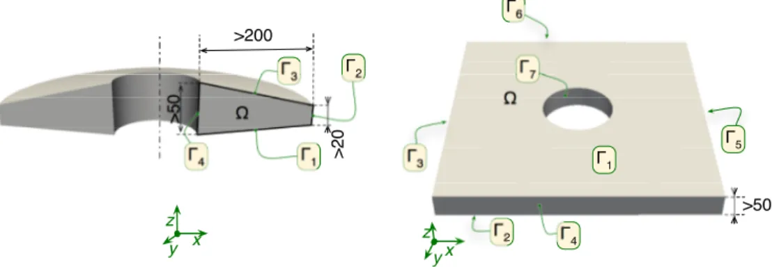
The coupled heat transfer and transformation problem is solved over a domainΩ the boundary of Ω, called Γ is the union of nb distinct boundaries:Γ = ∪ni=1b Γi. In the present study, two different geometries are considered: a three
dimensional complex part and a two dimensional axisymmetric part (see figure 1).
The domainΩ is considered large enough compared to the thickness of one ply. Thus, a homogenized behaviour is considered. For the sake of simplicity, the material is considered isotropic transverse in a global cartesian coordinate system. This comes down to considering a quasi-isotropic layup with a unique transverse direction.
Γ 3 Γ 2 Γ 4 Γ1 Ω Ω Γ 2 Γ4 Γ 3 Γ 6 Γ 7 z x y zyx >50 >5 0 >2 0 >200 Γ 5 Γ 1
FIGURE 1.DomainΩ studied. Simplified 2D case (left) and complex 3D geometry (right).
Heat transfer
Energy equilibrium
The heat conduction equation classically writes ρcp∂T
∂t = ∇ · (k∇T) + (1 − ϕ) ρmL ∂α
∂t (1)
where T is the temperature,ρ the density of the material, cpits specific heat capacity, k its conductivity tensor and∇
the spatial differential operator. The second term stands for the exotherm induced by the crystallization transformation: ϕ is the fibre volume content, ρmthe density of the matrix, L the apparent crystallization enthalpy, andα the degree of
transformation.
Initial and boundary conditions
The temperature in the domain is supposed initially uniform at T (t= 0) = T0> 300◦C.
The boundary condition onΓiare mixed with an outward flux q· n = hi
(
T− Timpi )
where q= −k∇T is the heat flux and n the outward normal vector. hiand Timpi depend on time t.
Degree of transformation
The polymer crystallization kinetics is classically modeled using the degree of transformationα that ranges between 0 when amorphous to 1 when maximum crystallinity is reached. The kinetics is typically ruled by an ordinary differential equation. Classical Nakamura [1, 2, 3] law writes
dα
dt = nKn(T ) g (α) (2)
where Kn(T ) is the kinetic function n the Nakamura index and
g(α) = (1 − α) [− ln (1 − α)]1−1n. (3)
As an initial condition, the material is considered full molten. Thusα should be equal to 0. Nonetheless, because equation (3) is singular in 0, we consider
NUMERICAL METHODS
The heat transfer problem is an evolution boundary value problem whereas the crystallization problem is a ordinary differential equation to be solved at each position. In this section standard numerical methods are proposed to handle this coupled problem. Then, in order to avoid numerical artifacts at the crystallization front, a special remeshing criterion is suggested.
Discretization
Spatial
The temperature field is discretized using a finite element method. This proved efficient to handle parabolic partial differential equations of the form of eq. (1). For the coherence of the scheme and to ease the implementation the degree of crystallization fields is also discretized using finite elements. The fields thus write successively
T(x, t) = {Ni(x, t)}T· {Ti(t)} α (x, t) = {Ni(x, t)}T· {αi(t)}
where Niare the interpolation functions, i being the degree of freedom index. In order to treat the coupled heat transfer
and crystallization problems, the unknown is seek as a concatenation of both fields: {Xi(t)} = { Ti(t) αi(t) } . Temporal
Time integration is performed using a classical incremental method with an implicit first order scheme. The time dt is adapted in order to ensure that for every position in the domainΩ, the right hand side of equation (2) is such that:
1. it is not singular (close toα = 0). dt is chosen such that 2dt < 1/ d fdα 2. α does not exceed 1. dt is chosen such that 2dt < (1 − α) / f (α).
Weak form and resolution scheme
The heat transfer boundary value problem and the crystallization kinetics problem are written in a weak form, using two test functions T∗ andα∗. Using the Galerkin method, T∗ andα∗are chosen as Ni. The coupled problem then
classically reduces to seeking the zero of a residual function
R(X)= 0. (4)
This function is nonlinear. A standard iterative Newton-Raphson procedure is thus adopted to find its zero. The un-known Xk+1is found from Xkby solving the linear system
dR
dX (Xk). (Xk+1− Xk)= −R (Xk), (5)
where dR/dX is the tangent matrix of the system.
Remeshing
Issue with sharp fronts
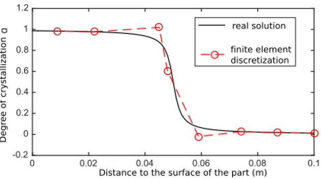
In the case of thick part, that can be several centimetres thick, the cooling rate can easily get below 5 K/min. The cooling cycles are thus long and the crystallization transformation zone is localized in small region compared to the part dimensions. As illustrated in figure 2, the degree of crystallizationα then presents a sharp front where it steeply increases from 0 to 1. As illustrated on the figure, in the case of a rough mesh, a standard finite element discretization of such a field is necessarily not accurate. The nodal value might locally become non physical (above 1 or below 0). An automatic remeshing, at the vicinity of the front, is thus necessary.
0 0.02 0.04 0.06 0.08 0.1 α Degr ee of cr ystallization -0.2 0 0.2 0.4 0.6 0.8 1 1.2 real solution finite element discretization
Distance to the surface of the part (m)
FIGURE 2.Illustration of the degree of crystallization field exhibiting a sharp front. A coarse finite element discretization cannot accurately predict represent the front.
Present work CAO Mesh GMSH Finite element solver FreeFem++ Post-treatment Paraview FreeFem script files Results files .mesh files STEP files Boundary conditions Material properties
FIGURE 3.Simulation framework. Several external tools are used for conducting a simulation. The present work is implemented in files illustrated in the central box.
Original remeshing criterion
To overcome this weak description, an remeshing algorithm is proposed. The remeshing criterion is such that the maximum of both Hessians of the temperature T and the degree of crystallizationα does not exceed a prescribed tolerance. It ensures a fine remeshing at the vicinity of the fields inflexions.
At a given time step, after the resolution of the coupled problems (equation (4)), remeshing is performed in two cases
1. If the field is not physical. Namely ifα < [α0, 1]. In that case the meshing tolerance is reduced and remeshing
is performed. The coupled problem is solved again for the same time step.
2. Every ten time iterations, the meshing criterion is increased and the remeshing is performed. This ensures mesh coarsening and front following while it moves in the domain.
Implementation
The global computation flowchart is illustrated in figure 3. The initial CAD geometry is first meshed using GMSH [4]. The finite element resolution is performed using FreeFem++ [5]. The hessian computation for remeshing criterion is done with the MshMet module and remeshing is automated with MMG3D [6].
In the three dimensional case, because of the high number of degrees of freedom (it can reach 1 million). The assembling and resolution of equation (5) is performed in parallel. After each remeshing, METIS is used for partition-ning [7]. The linear system parallel solver is MUMPS [8].
FIGURE 4.Temperature field computed in the 3D geometry at time t= 7000 s.
crist3D.jpg
FIGURE 5.Crystallization field computed in the 3D geometry at time t= 8000 s. The inset shows a detail of the fine remeshing at the vicinity of the crystallization front.
RESULTS
3D test case
A three dimensional test case representative of an industrial process was computed. The exchange coefficients are taken high (hi = 2000 Wm−2K−1) such that the boundary condition corresponds to an imposed temperature. These
different imposed temperatures Timpi (t) are adapted from experimental measurements and thus follow an real tabulated cycle. The cooling rate is not far from 2◦C/min but slightly differs between the different boundaries Γi.
Simulations was performed on a 64 cores cluster in parallel. The number of degrees of freedom varies with the remeshing but usually reaches about one million. The full transient nonlinear coupled problem is solved in a about 72 hours.
The temperature field at time t = 7000 s is represented in figure 4. On the left hand side, the field in the mid-surface shows that the core temperature is higher and that the central hole tooling helps cooling down the part.
The degree of crystallization field at time t = 8000 s is represented in figure 5. Solidification is initiated at the central hole surface which is the coldest part. The inset in the figure shows a detail of the fine remeshing at the vicinity of the solidification front.
2D benchmark
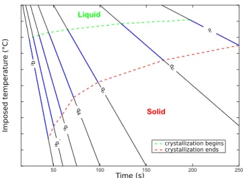
2D axisymmetric simulation (such as the one shown in figure 1) usually supposes a simplification of the real complex industrial geometry. Thus, it cannot reproduce fine three dimensional local effects. Nonetheless, it proves useful to quickly investigate the effect of process parameters. As an illustration, cases with different cooling rates (q1 < q2 <
... < q7) were simulated for the geometry given in figure 1. One simulation takes about 10 minutes on a desktop
computer. In figure 6 the imposed mould temperatures are plotted versus time. For each case, one can identify the point that correspond to the first solid germ at the cold mould contact (the liquidus) and the last liquid drop at the material core (the solidus). The transformation area can thus be plotted on this same graph. This is the continuous
50 100 150 200 250 Imposed temper atur e (°C ) q 1 q 2 q 3 q 4 q 5 ° q 6 q 7 Liquid Solid Time (s) crystallization begins crystallization ends
FIGURE 6.Continuous cooling diagram. Imposed temperature versus time. The blue area represents the range when transforma-tion occurs.
cooling transformation diagram.
CONCLUSION
The heat transfer and crystallization phenomena occurring during the forming of thick thermoplastic composite parts were simulated. This work is applicable, for instance, for investigating the cooling phase during injection moulding, or compression moulding. During thick part cooling and solidification a sharp crystallization front usually appear. The major contributions of this work are the following.
• A specific simulation framework for the coupled heat transfer and crystallization kinetics was proposed. • A remeshing criterion and algorithm permits an accurate description of the sharp front.
• Parallel implementation permitted simulation on complex 3D shapes case.
• A screen investigation of the process was performed using batch two dimensional simulations.
ACKNOWLEDGEMENTS
This study was made possible through the financial support provided by Airbus Helicopter, and DGA. The authors would like to thank Maxime Villi`ere who performed an extensive material characterization campaign that fed the model. Nathalie Robert also helped with the parallelization and installation on the university cluster.
REFERENCES
[1] K. Nakamura, T. Watanabe, K. Katayama, and T. Amano, Journal of Applied Polymer Science 16, 1077–1091 (1972).
[2] E. Quinlan, “Thermal and crystallinity profiles in laminates manufactured with automated thermoplastic tow placement process,” Ph.D. thesis, McGill University 2011.
[3] X. Tardif, B. Pignon, N. Boyard, J. W. Schmelzer, V. Sobotka, D. Delaunay, and C. Schick, Polymer Testing 36, 10–19 (2014).
[4] C. Geuzaine and J.-F. Remacle, “GMSH, a three-dimensional finite element mesh generator with built-in pre-and post-processing facilities,” .
[5] F. Hecht, Journal of Numerical Mathematics 20, 251–265 (2012).
[6] J. Morice, C. Drobrzynski, and P. Frey, “3D Metrics Tools : Mshmet and 3D Meshing Tools : Mmg3D and Freeyams,” in FreeFem days (2010), pp. 1–15.
[7] G. Karypis and V. Kumar, SIAM Journal on Scientific Computing 20, 359–392 (1998).