Spectrum sensing techniques in cognitive wireless sensor networks

(1)

HAL Id: tel-01399124

https://hal.archives-ouvertes.fr/tel-01399124

Submitted on 18 Nov 2016

HAL is a multi-disciplinary open access

archive for the deposit and dissemination of sci-entific research documents, whether they are pub-lished or not. The documents may come from teaching and research institutions in France or abroad, or from public or private research centers.

L’archive ouverte pluridisciplinaire HAL, est destinée au dépôt et à la diffusion de documents scientifiques de niveau recherche, publiés ou non, émanant des établissements d’enseignement et de recherche français ou étrangers, des laboratoires publics ou privés.

Public Domain

networks

Shaoyang Men

To cite this version:

Shaoyang Men. Spectrum sensing techniques in cognitive wireless sensor networks. Electronics. UNI-VERSITE DE NANTES, 2016. English. �tel-01399124�

(2)

Thèse de Doctorat

Shaoyang MEN

Mémoire présenté en vue de l’obtention du

grade de Docteur de l’Université de Nantes

sous le sceau de l’Université Bretagne Loire

École doctorale : Sciences et technologies de l’information et mathématiques (STIM) Discipline : Electronique

Spécialité : Communications numériques Unité de recherche : IETR UMR 6164 Soutenue le 27 Octobre 2016

Spectrum sensing techniques in cognitive

wireless sensor networks

JURY

Président : M. Tanguy RISSET, Professeur, Insa-Lyon

Rapporteurs : M. Emanuel RADOI, Professeur, Université de Bretagne Occidentale

M. Mohammad-Ali KHALIGHI, Maitre de conférences HDR, École Centrale de Marseille

Directeurs de thèse : M. Sébastien PILLEMENT, Professeur, École Polytechnique de l’Université de Nantes

(3)

(4)

Acknowledgments

First of all, I would like to express my sincere gratitude to my supervisors Prof. Sébastien Pillement and Prof. Pascal Chargé for their patient guidance, constant en-couragement and professional advice throughout the entire three years of my PhD study. I have been extremely lucky to work with so great supervisors who cared so much about my research work, who responded to my questions so promptly, and who spent countless hours correcting the manuscripts.

I would also like to thank Prof. Yide Wang, for his helpful suggestions and encour-agement.

Of course, I have to thank the jury, for their patient review and for taking them too much time.

In addition, I am sincerely grateful for all the help of Marc Brunet, Sandrine Charlier and all the other members of staff in IETR laboratory of Polytechnique de L’Université de Nantes.

I also want to thank my friends, we really had a wonderful time for my PhD life in France.

Finally, I must express my gratitude to my parents and my wife, for their continued support and encouragement.

(5)

(6)

Résumé de la thèse en français

Aujourd’hui, avec le développement rapide des technologies de communication sans fil, des services de plus en plus nombreux apparaissent dans tous les aspects de notre vie tels que les soins de santé, les bâtiments intelligents, la surveillance du trafic, l’observation de champs de bataille, des applications multimédias. Le spectre étant considéré comme une ressource limitée, il en résulte une compétition croissante entre les applications sans fil. En outre, en raison de la stratégie d’allocation du spectre fixée par l’autorité de régulation, la plupart des bandes de fréquences sont a priori réservées pour certains utilisateurs agréés. Par exemple, la gamme de fréquences comprise entre 512 MHz et 608 MHz est attribuée aux canaux de télévision 21-36. Il n’existe que très peu de bandes libres dans le spectre électromagnétique exploitable par les applications sans fil. De plus, les bandes réservées semblent ne pas être pleinement exploitées; de manière inattendue le taux d’utilisation du spectre semble être de moins de 30% [1].

Afin de faire face à la rareté et à la sous-exploitation des ressources spectrales, des stratégies de partage du spectre ont été proposées. L’idée de base est de permettre à chacun d’utiliser le spectre sous licence lorsqu’il n’est pas occupé par son propriétaire officiel (utilisateur primaire). L’utilisateur secondaire n’est donc pas prioritaire et ne

doit causer aucune interférence à l’utilisateur primaire [2, 3, 4, 5]. Les technologies

de radio cognitive [6], se sont imposées dans cette stratégie, en utilisant un mécanisme de cognition pour détecter le spectre, déterminer des groupes vacants et utiliser ces

bandes disponibles de manière opportuniste [7, 8]. La première étape du cycle de

la cognition est la détection du spectre, elle joue un rôle essentiel et central dans la radio cognitive. L’utilisateur cognitif (utilisateur secondaire) doit détecter rapidement et de manière certaine que l’utilisateur autorisé est présent ou non dans une bande de fréquence considérée. Il existe diverses méthodes de détection de spectre pour la radio

cognitive dans la littérature [9,10], mais très peu d’entre elles semblent être vraiment

appropriées au contexte des réseaux cognitifs de capteurs sans fil.

Les réseaux cognitifs de capteurs sans fil sont définis comme des réseaux distribués de nœuds cognitifs de capteurs sans fil. Généralement conçus pour relever des mesures

(7)

ou détecter des événements, les nœuds capteurs du réseau collaborent entre eux et com-muniquent dynamiquement sur les bandes de fréquences disponibles. Un réseau cog-nitif de capteurs sans fil possède donc des capacités cognitives pour l’exploitation du spectre [11]; ce qui n’est pas le cas des réseaux sans fil traditionnels. Par conséquent, les nœuds de capteurs sans fil sont équipés de la capacité cognitive. Les avantages at-tendus sont multiples: (1) Utilisation plus efficace du spectre: Les nœuds des réseaux de capteurs sans fil existants utilisent généralement une bande fixe sans licence pour communiquer. Ces bandes libres sont donc en général très fréquentées par d’autres appareils. Par conséquent, l’accès au spectre de manière opportuniste est en mesure d’améliorer la cohabitation efficace des plusieurs utilisateurs/services. (2) Plusieurs canaux de communication potentiels: Dans les réseaux de capteurs sans fil à forte densité de déploiement, un grand nombre de nœuds de capteurs tentent d’accéder au même canal en même temps. Cela augmente la probabilité de collisions et de pertes de paquets, ce qui diminue la fiabilité globale de communication avec une consommation d’énergie excessive. Les réseaux cognitifs de capteurs sans fil ont en revanche la ca-pacité d’exploiter plusieurs canaux selon leur disponibilité de façon opportuniste pour atténuer ces problèmes potentiels. (3) Efficacité énergétique: Les réseaux cognitifs de capteurs sans fil sont en mesure de modifier leurs paramètres de fonctionnement selon les conditions du canal afin d’optimiser leur consommation d’énergie liée aux trans-mission. (4) Opérabilité mondiale: La réglementation d’exploitation du spectre peut être différente d’une région à une autre, certaines bandes sont libres dans une région tandis qu’elles ne sont pas exploitables dans un autre pays. Les réseaux de capteurs cognitifs peuvent s’adapter à n’importe quelle réglementation grâce à l’agilité spectrale des nœuds cognitifs.

Cependant, la réalisation de réseaux cognitifs de capteurs sans fil et les avantages potentiels ci-dessus nécessitent de répondre à certains défis. En général, un nœud cog-nitif de capteurs sans fil se compose de cinq éléments de base: une unité de détection-capteur, une unité de traitement et de stockage, une unité dite de traitement-décision dédiée aux fonctions radio-cognitives, un module radio émetteur-récepteur et une ali-mentation. Souvent imposé par le contexte d’application, le nœud doit généralement répondre à de nombreuses contraintes (limitation de la consommation, capacité de cal-cul, durée de vie, la durée de détection, fiabilité des mesures . . . ). Notamment, les nœuds sont parfois situés dans des endroits inaccessibles, ce qui exclut le remplace-ment des piles et entraine dans ce cas que l’une des principales préoccupations pour l’exploitation du réseau cognitif est la consommation d’énergie. Parmi les composants des nœuds de capteurs, l’unité radio émetteur-récepteur consomme beaucoup d’énergie

(8)

afin de fournir une connectivité aux autres nœuds. En outre, le traitement et la mémoire sont également limités. En raison des contraintes de coût et de taille, les capacités de traitement des nœuds peuvent s’avérer relativement limitées par rapport à d’autres sys-tèmes embarqués [12]. Cependant, les différentes méthodes existantes de détection du spectre pour la radio cognitive dans la littérature ne considèrent pas ces limites de ressources des nœuds de capteurs. Par conséquent, concevoir une technologie spéci-fique de radio cognitive pour les réseaux cognitifs de capteurs sans fil est un sujet non résolu.

Dans le chapitre 2, nous présentons les techniques de détection de spectre dévelop-pée dans la littérature. Ce chapitre reprend aussi les indicateurs de performance qual-ifiant ces techniques. La détection du spectre peut se faire uniquement localement au niveau de chaque nœud (détection locale), ou de manière coopérative entre plusieurs nœuds du réseau (détection coopérative). Dans le cas de la détection locale du spec-tre, nous présentons plusieurs méthodes basées sur les principes suivants: détection de l’énergie, la détection à base de valeurs propres de la matrice de covariance des obser-vations, test du Goodness-of-Fit etc.. Concernant la détection coopérative du spectre, nous discutons de la détection du spectre de coopération centralisée et la détection du spectre coopératif distribuée. Ensuite, nous nous concentrons sur la présentation des méthodes de fusion. Il s’agit de générer une décision en combinant les données issues des nœuds, à partir de règles (hard decision, soft decision, théorie des croy-ances de Dempster-Shafer, etc.). Cependant, comme indiqué dans le chapitre 2, la plupart de ces méthodes ont leurs limitations. Par exemple, la détection d’énergie per-met d’atteindre une bonne performance de détection uniquement lorsque la taille de l’échantillon est suffisamment grande [13]. De même, de nombreuses méthodes de détection basées sur l’analyse des valeurs propres de la matrice de covariance ont été

proposées [14,15,16,17,18], mais la plupart d’entre elles ont des exigences intenables

en termes de durée d’observation (ce qui génère une grande taille de l’échantillon) et de complexité de calcul.

Considérant les contraintes et les limitations précédentes des méthodes de détection du spectre de la littérature, nous proposons d’étudier de nouvelles techniques permet-tant de détecter le spectre à partir d’un faible nombre d’échantillons. Cette caractéris-tique est en effet un moyen de limiter la consommation des circuits et la complexité des traitements. Un petit nombre d’échantillons permet de réduire considérablement la durée d’observation du spectre, ce qui se traduit aussi par une économie d’énergie et une prolongation de la durée de vie de l’ensemble du réseau.

(9)

méthode repose sur un modèle statistique des signaux reçus ainsi que sur l’utilisation de la théorie des croyances de Dempster-Shafer. Les échantillons du canal sont tout d’abord séparés en plusieurs groupes pour former une variable aléatoire pour chaque groupe. Le nombre d’échantillons étant faible, il apparaît que cette variable suit une loi t de Student. Les paramètres de cette loi sont différents selon que le canal ne com-porte que du bruit ou qu’il soit utilisé par un utilisateur primaire. Cette différence va

être exploitée pour distinguer les deux hypothèses (H0 absence d’utilisateur primaire

/ H1 présence d’un utilisateur primaire) en s’appuyant sur la théorie des croyances de

Dempster-Shafer. Ainsi pour chaque groupe d’échantillons, des BPA (Basic

Probabil-ity of Assignement) sont calculées pour les deux hypothèses: mi(H0)et mi(H1). Le

processus de fusion de Dempster-Shafer est ensuite utilisé pour produire une décision finale à partir des BPA de tous les groupes d’échantillons. Les résultats de simulation montrent que la probabilité de détection de la méthode proposée est supérieure aux autres méthodes locales de la littérature lorsque le nombre d’échantillons est faible.

Dans le chapitre 4, une méthode coopérative de détection du spectre est proposée. La technique repose aussi sur la théorie des croyances de Dempster-Shafer, mais le processus de fusion permettant d’obtenir la décision globale exploite les BPA fournies par chacun des nœuds du réseau. Cette fusion est faite au niveau d’un nœud particulier appelé centre de fusion. Au niveau de chaque nœud (utilisateur secondaire) il s’agit donc de calculer les BPA relatives aux deux hypothèses à partir d’un faible nombre d’échantillons. Pour cela, la technique s’appuie à nouveau sur un modèle statistique des observations. En effet, chaque utilisateur secondaire forme une matrice de co-variance de ses observations. Ici encore, le nombre d’échantillons pour calculer cette matrice de covariance est faible et de plus le taux d’échantillonnage est choisi rela-tivement faible de telle manière que les échantillons sont considérés indépendants. Il s’avère dans cette situation que la plus forte valeur propre de la matrice de covari-ance est régie par une loi statistique de Tracy-Widom. Comme précédemment, les paramètres de la loi sont différents selon que l’on soit en présence ou non d’un utilisa-teur primaire. Cette différence est exploitée au niveau de chaque utilisautilisa-teur secondaire pour calculer les BPA pour les deux hypothèses. Les résultats de simulation permettent de vérifier l’efficacité de la méthode proposée pour les faibles nombres d’échantillons. Dans le chapitre 5, une autre technique coopérative de détection du spectre est pro-posée. L’approche est différent du chapitre précédent car les critères privilégiés sont ici la consommation et la fiabilité de la décision. Dans un premier temps l’organisation du réseau en cluster est étudiée. Les nœuds (utilisateurs secondaires) sont donc regroupés en clusters de manière à réduire la consommation globale liée aux communications

(10)

pour effectuer la détection coopérative à l’échelle du cluster. Basé sur l’algorithme K-mean, la technique de formation du cluster permet aussi de désigner le meilleur nœud centre de fusion pour la détection de spectre dans le cluster. Ensuite la méthode de détection de spectre consiste à mettre en œuvre un double critère de fiabilité des util-isateurs. La théorie des croyances de Dempster-Shafer est une nouvelle fois utilisée pour qualifier les deux hypothèses des utilisateurs secondaires et combiner ces infor-mations au niveau du centre de fusion du cluster. La technique repose d’une part sur une estimation du niveau de bruit reçu par chaque utilisateur et d’autre part sur le sou-tien mutuel que s’accordent les utilisateurs entre eux. De cette manière un utilisateur évoluant dans un milieu trop bruité verra sa crédibilité diminuer, et de même un util-isateur fournissant des BPA trop différentes des autres verra aussi baisser sa crédibilité (soutien mutuel). Enfin, les utilisateurs dont la crédibilité est trop basse sont rejetés du processus de fusion pour la décision globale dans le cluster. Ce principe permet d’améliorer la fiabilité de la décision car les utilisateurs secondaires les moins crédi-bles ne participent pas à la décision. Un utilisateur peut être considéré non crédible par exemple lorsque sa perception du canal est trop mauvaise ou simplement lorsqu’il est défectueux. Des résultats de simulation sont fournis pour illustrer les performances du système proposé.

La thèse se termine par une conclusion reprenant les différentes contributions et indiquant quelques perspectives.

(11)

(12)

List of Figures

1.1 A snapshot of spectrum utilization where each band averaged over 6

locations [1]. . . 20

1.2 Cognition cycle. . . 22

2.1 The classification of spectrum sensing techniques. . . 28

2.2 Illustration of the ROC curve in [19]. . . 30

2.3 Local spectrum sensing techniques. . . 31

2.4 Block diagram of matched filter detection [19]. . . 32

2.5 Block diagram of cyclostationary feature detection. . . 36

2.6 Block diagram of energy detection. . . 37

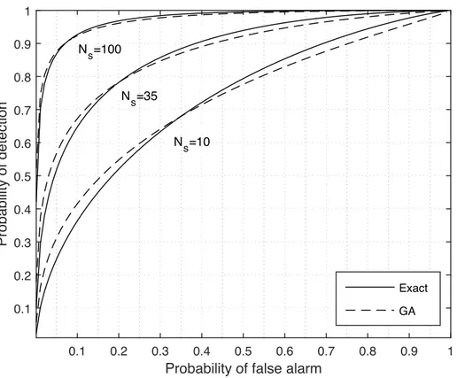
2.7 The ROC comparison of ED for the exact chi-squared model and the Gaussian approximation model. . . 40

2.8 Sensing accuracy and complexity of various sensing methods [20, 21]. 50 2.9 Block diagrams of traditional Nyquist wideband sensing based on multi-band joint detection [22]. . . 50

2.10 The diagram of centralized cooperative spectrum sensing. . . 53

2.11 The diagram of distributed cooperative spectrum sensing. . . 54

3.1 Histogram and the GoF of Zjunder H0hypothesis with only noise and H1 hypothesis with signal plus noise. . . 68

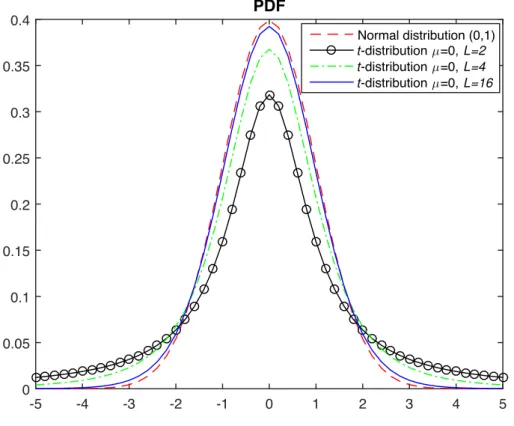
3.2 The impact of the different degrees of freedom v = L 1 for the probability density function (PDF) of student’s t-distribution. . . 69

3.3 The tendency of the BPA functions of Zj including mj(H0)under H0 hypothesis and mj(H1)under H1 hypothesis. . . 71

3.4 Probability of detection versus SNR for the proposed method and ED with different sampling numbers. . . 74

3.5 ROC curves of the proposed method and ED with different sampling numbers at SNR= -6 dB. . . 75

(15)

3.6 ROC curves comparison among different spectrum sensing methods with Ns= 16samples. . . 76 4.1 Scenario and framework of cooperative spectrum sensing in CWSNs. 81 4.2 Comparison of eigenvalues between theoretical value and simulative

value where there are a finite number of samples. (a) Only noise in H0 hypothesis. (b) Signal plus noise in H1hypothesis. . . 84 4.3 Comparison of the theoretical CDF of the maximum eigenvalue, TW

distribution and adjusted TW distribution with Ns = 50and L = 4.. . 87 4.4 The tendency of the BPA functions of ( 1i µi)/ i under H0 and H1

hypotheses. . . 89 4.5 The variation trend of the BPA functions with the increasing of SNR

when PU is present using 200 samples. . . 91 4.6 The variation trend of the BPA functions with the increase of SNR

when PU is present using 50 samples. . . 92 4.7 ROC curves of the compared methods using 200 samples at each SU. 93 4.8 ROC curves of the compared methods using 50 samples at each SU. . 94 4.9 ROC curves of our proposed scheme with different numbers of SU

when the sample number is 50. . . 95 5.1 Cluster-based cooperative spectrum sensing in CWSNs where some

faulty nodes are existing. . . 99 5.2 The energy efficiency performance for different cluster number. . . . 107 5.3 100 SUs are scattered into 8 clusters with K-means clustering algorithm.108 5.4 Probability of detection comparison between proposed algorithm and

other methods.. . . 109 5.5 Probability of detection comparison of proposed double reliability

eval-uation algorithm. . . 110 5.6 Energy consumption in each cluster from C1 to C8. . . 111

(16)

List of Symbols

2 _{. . . Chi square distribution}

. . . Signal to noise ratio

max . . . Maximum eigenvalue

min . . . Minimum eigenvalue

2

w . . . Variance of noise

⇣ . . . Threshold

m . . . Basic probability assignment function

Ns . . . Number of samples

Nsu . . . Number of secondary users

Pd . . . Probability of detection

Pf a . . . Probability of false alarm

Pm . . . Probability of miss

H0 . . . Hypothesis of only noise

H1 . . . Hypothesis of signal plus noise

N . . . Gaussian distribution T . . . Test statistic

(17)

(18)

List of Abbreviations

AWGN . . . Additive White Gaussian Noise BPA . . . Basic Probability Assignment CDF . . . Cumulative Distribution Function CFD . . . Cyclostationary Feature Detection CR . . . Cognitive Radio

CSS . . . Cooperative Spectrum Sensing CWSNs . . . Cognitive Wireless Sensor Networks D-S . . . Dempster-Shafer

EBS . . . Eigenvalue Based Sensing ED . . . Energy Detection

FC . . . Fusion Center GoF . . . Goodness of Fit

LSS . . . Local Spectrum Sensing MFD . . . Matched Filter Detection

MME . . . Maximum Minimum Eigenvalue PDF . . . Probability Density Function PU . . . Primary User

ROC . . . Receiver Operating Characteristic SNR . . . Signal to Noise Ratio

SS . . . Spectrum Sensing SU . . . Secondary User TW . . . Tracy Widom

WBS . . . Waveform Based Sensing WSNs . . . Wireless Sensor Networks

(19)

(20)

1

Introduction

1.1 Background

Nowadays, with the rapid development of wireless communication technology, more and more wireless services are used in all aspects of life such as health care, intelligent buildings, vehicle traffic monitoring, battlefield surveillance, multimedia applications and so on. The limited spectrum resource can not meet the growing de-mand of wireless application. In addition, due to the existing fixed spectrum allocation strategy, most frequency bands are specified for the licensed user (LU) where the other communication device is not allowed to utilize it in spite of the unoccupied band. For example, the frequency range between 512 MHz and 608 MHz is assigned as TV chan-nel 21-36, which means that only TV user can use it, but the others can not occupy it at any time. A mass of allocated frequency bands cause that the available spectrum is so little. Even more unfortunately, the spectrum utilization rate of LU are unexpectedly

under 30% [1], as shown in Figure1.1. The fixed mobile frequency band 1850-1990

MHz and the air traffic control frequency band 108-138 MHz are even used at 5%. In order to solve the scarcity of spectrum resource and the low spectrum utiliza-tion, dynamic spectrum allocation (DSA) which is a flexible and intelligent spectrum management mode has been proposed [2]. In DSA, according to the actual require-ments of wireless communication system, spectrum resource is dynamically allocated to those wireless systems. When this process is finished, the spectrum is taken back by

(21)

Figure 1.1 – A snapshot of spectrum utilization where each band averaged over 6 locations [1].

the assignment system. Although this management mode is efficient for the spectrum utilization, it changed the current static frequency allocation schemes. Therefore, spec-trum sharing strategy without altering the current frequency allocation schemes which is considered as the popular spectrum sharing technique has been proposed. The basic idea is to open licensed spectrum to unlicensed users while limiting the interference perceived by licensed user. It mainly includes two approaches to spectrum sharing: spectrum underlay and spectrum overlay [3].

The spectrum underlay approach allows that the unlicensed user accesses the li-censed spectrum with a extremely low power, which results in multiple communica-tion system using the same frequency band simultaneously [4]. Due to the very low power of the unlicensed user, like a background noise for the licensed user, there is no serious interference with the licensed user when the licensed and unlicensed users exe-cute their own operations at the same time under the same frequency band. According to this, the unlicensed ultra-wideband (UWB) working in the frequency range from 3.1 GHz to 10.6 GHz, whose power spectrum density emission is limited -41.3 dBm/MHz, can coexist with the worldwide interoperability for microwave access (WiMAX) at 3.5 GHz band [5]. On the other hand, the spectrum overlay approach does not necessarily impose severe restrictions on the transmission power of unlicensed users, but rather on when and where they may transmit. In other words, when the licensed frequency band

(22)

is unoccupied at spatial and temporal scales, the unlicensed user is allowed to operate in the frequency band. In this spectrum overlay, two approaches including opportunity spectrum sharing and cooperation spectrum sharing are considered.

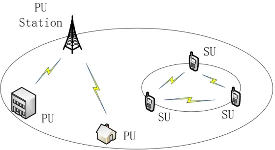
In cooperation spectrum sharing, the licensed user needs to know whether the un-licensed user is present or not. And when the un-licensed user prepares working, if the unlicensed user is using the licensed frequency band, the licensed user chooses the other unoccupied sub-channels for operating and does not interrupt the communica-tion of the unlicensed user. In opportunity spectrum sharing, it does not know the situation of the unlicensed user and has no cooperation between the licensed and unli-censed user. When the unliunli-censed user needs to access the liunli-censed frequency band, it needs to detect whether the licensed user is present or absent. If the licensed frequency is occupied by the licensed user, the unlicensed user can not access the spectrum; otherwise, it can use the licensed spectrum. When the licensed user reoccupies the frequency band, the unlicensed user needs to quit immediately and look for a new un-occupied frequency band. Therefore, this approach is sufficient for Cognitive Radio (CR) which is first proposed by Mitola [6] and is defined by Federal Communications Commission (FCC) as : “A radio or system that senses its operational electromagnetic environment and can dynamically and autonomously adjust its radio operating param-eters to modify system operation, such as maximize throughput, mitigate interference, facilitate interoperability, access secondary markets." [7].

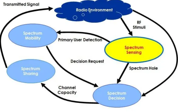
CR utilizes a mechanism called cognition cycle as shown in Figure 1.2 [8] for

sensing the spectrum (spectrum sensing, SS), determining the vacant bands (spectrum decision) and making use of these available bands in an opportunistic manner (spec-trum mobility and spec(spec-trum sharing). As the first step of cognition cycle, spec(spec-trum sensing plays an essential and central role in CR. The key of SS is that the cognitive user (as the secondary user, SU) needs to detect quickly and reliably that the licensed user (as the primary user, PU) is present or not in a considered frequency band. There

are various method of spectrum sensing for CR in the literature [9,10], but a very few

of them seem to be really suitable in the context of cognitive wireless sensor networks (CWSNs).

CWSNs is defined as distributed networks of wireless cognitive radio sensor nodes, which sense event signals and collaboratively communicate their readings dynami-cally over available spectrum bands in a multihop manner to ultimately satisfy the application-specific requirements [11], which can be constructed by incorporating CR technology into the traditional wireless sensor networks (WSNs). Therefore, the sen-sor nodes in WSNs are equipped with cognitive ability, which may benefit the WSNs.

(23)

Figure 1.2 – Cognition cycle.

The advantages of using CR in WSNs are discussed in the following:

• Efficient spectrum utilization: Current WSNs are deployed over unlicensed frequency band, such as industrial, scientific and medical (ISM) radio bands, which faces an increased level of interference from various wireless system. ISM bands are overcrowded which limits the development of new technologies. Dy-namic spectrum access in CR is able to make SU cooperate efficiently with other types of users.

• Multiple channels utilization: In traditional WSNs referring to the detection of an event, several sensor nodes generate bursty traffic. Especially, when in densely deployed WSNs, a large number of sensor nodes attempt to access the same channel at the same time. It increases the probability of collisions and packet losses, which decreases the communication reliability with exces-sive power consumption. CWSNs access multiple channels opportunistically to alleviate these potential challenges.

• Energy efficiency: CWSNs may be able to change their operating parameters according to the surrounding channel conditions in order to avoid the power waste for packet retransmission due to packet losses in traditional WSNs. • Global operability: Due to different spectrum regulations, a certain band in one

(24)

specific region or country may be available, while it is not available in another places. However, the sensor nodes with cognitive capability in CWSNs may overcome this potential problem.

However, the realization of CWSNs and the potential advantages above depends on addressing some challenges that are introduced by the wireless sensor node equipped with cognitive capability in CWSNs. Generally, a cognitive wireless sensor node con-sists of five basic units: a sensing unit, a processing and storage unit, a CR unit, a transceiver unit and a power unit. Just like a traditional wireless sensor node, it has hardware constrains in terms of computational power, storage and energy. Therefore, considering the limitation of processing, memory and energy, it is still a serious chal-lenge to design specific CR technology in CWSNs.

1.2 Motivation

It is provided that the cognitive wireless sensor node in CWSNs is resource con-strained that refers to power limitation, hardware limitations, sensing duration and reliability. Because most WSNs are inaccessible or it is not feasible to replace the bat-teries of the node when the limited battery power is exhausted, the main concern for the operation of CWSNs is the energy consumption. Among the components of sensor nodes, the transceiver unit consumes the most energy in order to provide connectivity to the other nodes. In addition, the processing and memory are also constrained. Due to the cost and size constraints, the processing power of current nodes is seriously lower than the other embedded systems [12]. However, the existing various methods of spec-trum sensing for CR in the literature do not consider these limits of resource of sensor nodes. For example, energy detection is able to achieve a good detection performance only when the sample size is sufficiently large [13]. Numerous covariance matrix or

eigenvalue based detection methods have been proposed in [14,15, 16,17, 18], most

of them have the requirements of the long sensing time (large sample size) and the high computational complexity.

Motivated by the constrained resource described and the limitation of the existing spectrum sensing methods above, as a way of solving this problem, small sample size is proposed to design new efficient CR techniques, especially in spectrum sensing al-gorithms, which is able to preferably adapt in CWSNs. A small number of samples can greatly reduce the data burden of the transceiver unit, which results in an exciting energy saving. Due to the most energy consumed by the transceiver unit as shown

(25)

above, small samples size plays a role to prolong the usage of sensor nodes and even extend the lifetime of the whole network. Besides, it also alleviates the limits of the processing power and memory. Therefore, small sample size is an efficient method to adopt in CWSNs where sensor nodes are resource constrained and additional CR actions is required.

In order to cope with the small sample size, we firstly propose to reformulate the spectrum sensing into a student’s t-distribution test problem. It is demonstrated that the student’s t-distribution test under small sample size can also provide a low error rates close to the 5% nominal value [23]. Thus, according to this characteristic of stu-dent’s t-distribution and taking into account several goodness of fit (GoF) tests [24], an efficient local spectrum sensing method is proposed on basis of both hypotheses of presence and absence of PU signal, which is able to get a high reliability of detection. However, in order to focus on dealing with the small sample size, we do not consider the channel condition in the system model of the proposed method. Hence, consider-ing the SU practically experiencconsider-ing path loss, multipath and shadowconsider-ing, we propose to adopt a cooperative spectrum sensing strategy based on multiple sensor nodes in order to improve the reliability of detection, which is based on an adjusted Tracy-Widom distribution that is suitable for small sample size. In summary, two solutions to small sample size including the student’s t-distribution and the adjusted Tracy-Widom dis-tribution are proposed at the beginning.

However, small sample size really increases the uncertainty of the observation sam-ples and reduces the reliability of final decision. Therefore, our efforts begin with the Dempster-Shafer (D-S) theory of evidence that can deal with the uncertainty from the small observation samples and improve the reliability by fusing different data groups. According to the D-S theory of evidence, after coping with the small number of sam-ples, some basic probability assignment (BPA) are estimated with the characteristic of the student’s t-distribution or the adjusted Tracy-Widom distribution. Finally, relying on the fusion of different probability assignment estimations, we make a reliable fi-nal decision whether a PU sigfi-nal is present or not. These refer to the proposed local spectrum sensing (LSS) based on the GoF principle and cooperative spectrum sensing (CSS) based on D-S theory of evidence.

In addition, the energy efficiency of the whole network and the reliability of the decision are also great challenges. On the one hand, an unreasonable allocation of sensor nodes in the network can result in a great waste of the transmission power among sensor nodes. On the other hand, it is necessary to consider the security issues of sensor nodes in the whole networks. For example, sometimes some nodes inevitably

(26)

fail in sending the information data due to battery depletion, electronic device under harsh environment or even being attacked by malicious users. Considering the situation mentioned above, a robust and energy efficient cooperative spectrum sensing scheme is proposed, which is based on a clustering algorithm and utilizes a double reliability evaluation.

1.3 Contributions

The main contributions of this thesis are summarized as follows.

• An efficient local spectrum sensing with small sample size is proposed. In the proposed method, we reformulate spectrum sensing into a student’s t-distribution test problem and propose some new basic probability assignment evaluations. Then, the D-S theory of evidence is used to make a decision relying on both hypotheses of presence or absence of PU. Simulation results show that the pro-posed method can achieve a higher probability of detection than other compared methods with small sample size.

• An efficient cooperative spectrum sensing with small sample size is proposed. In the proposed method, considering the channel condition at each SU, a more reasonable Tracy-Widom approximation is utilized to form a thin observation matrix. Then, we also propose some new BPA functions based on the largest eigenvalue of the received sample covariance matrix, which considers the credi-bility of local spectrum sensing. Finally, a more reliable final decision is made. Simulation results verify the effectiveness of the proposed method for small sam-ple size scenarios.

• A robust and energy efficient cooperative spectrum sensing scheme in CWSNs is proposed. In the proposed method, firstly, considering the energy consump-tion of sensor nodes, we propose a cluster-based cooperative spectrum sensing scheme where the energy consumption of the communications unit for the SU is reduced extremely and the spectrum utilization of the spectrum hole for the whole network is remarkably improved. Secondly, taking the reliability problem into account, we propose a method that allows to consider simultaneously the reliability of each SU in the cluster and the mutually supportive degree among the whole set of SUs in the cluster, namely double reliability evaluation. Finally, after removing the nodes of low credibility, the energy efficiency and reliabil-ity of each cluster is improved. Simulation results show that the proposed CSS

(27)

scheme clearly allows to save energy and provides a more robust decision under faulty nodes situation.

1.4 Outline of the thesis

The remainder of this thesis is organized into five chapters as listed below.

• Chapter 2 overviews the developed spectrum sensing techniques in the literature. At first, the performance indicators of spectrum sensing techniques are given. Then, we discuss the local spectrum sensing techniques, where several local spectrum sensing methods such as energy detection, eigenvalue based sensing, GoF test based sensing, etc. are presented. After that, we introduce the coop-erative spectrum sensing, which includes the centralized coopcoop-erative spectrum sensing and the distributed cooperative spectrum sensing. We focus on present-ing fusion methods such as hard-decision, soft-decision combinpresent-ing data fusion schemes, bayesian fusion rule, D-S theory of evidence, etc..

• Chapter 3 presents the proposed local spectrum sensing with small sample size. First of all, we take advantage of the student’s t-distribution to cope with the small number of samples. Then some new basic probability assignment func-tions are proposed in order to evaluate the reliability of observation samples. At last, the D-S theory of evidence is used to make a decision. The simulation results referring to the performance comparisons are also given.

• Chapter 4 presents the proposed cooperative spectrum sensing with small sam-ple size. At the beginning, the system model considering channel conditions is given. We then consider an adjusted Tracy-Widom distribution and use the eigenvalue based method at each SU. After that, we estimate the reliability of each SU and combine these results to make a final decision using D-S theory of evidence. Some simulation results and analyses are given at the end.

• Chapter 5 introduces the proposed robust and energy efficient cooperative spec-trum sensing scheme in CWSNs where some faulty nodes are existing. On one hand, we make use of the clustering algorithm in the whole network. On the other hand, a double reliability evaluation is presented in each cluster to remove the nodes of low credibility. We also show the simulation results of each method and give the performance comparisons with other methods.

• Chapter 6 gives the conclusions of this thesis and the possible directions in the future work.

(28)

2

Overview of spectrum sensing

techniques

In order to improve spectrum efficiency and alleviate the problem of spectrum re-sources constraints, the concept of cognitive radio is proposed which is a smart wireless communication system. A cognitive radio is able to be aware of its environment and learn from the surrounding, then change the corresponding operating parameters, such as transmission power, carrier frequency, its modulation mode, etc., finally in real time adjust the internal state of cognitive radio user to accommodate the impending change in radio frequency excitation [25].

In cognitive radio, a major challenge is that the SU needs to sense the presence of PU in a licensed frequency band, and to leave it as quickly as possible when the PU emerges in order to avoid interference to the PU. This technique is called spectrum sensing. As a critical part of CR, spectrum sensing has attracted a large amount of interest and several spectrum sensing techniques have been widely studied in the

liter-ature [9,10,20,21]. According to whether the sensing needs collaboration or not, we

can classify all spectrum sensing algorithms into two main types: local and

coopera-tive spectrum sensing, (as shown in Figure2.1). In local spectrum sensing, the detector

makes a decision only on basis of its own sensing, whereas cooperative spectrum sens-ing is able to use multiple devices and combine their measurements to make a decision.

Those techniques are briefly explained in Section2.2and Section2.4, respectively.

(29)

Spectrum Sensing Algorithms Cooperative Spectrum Sensing Local Spectrum Sensing

Figure 2.1 – The classification of spectrum sensing techniques.

Before exploring local spectrum sensing and cooperative spectrum sensing, we

describe performance indicators of spectrum sensing techniques in Section2.1.

2.1 Performance indicators of spectrum sensing

tech-niques

Before showing the performance indicators of spectrum sensing techniques, the general signal detection model and decision criterion are described. The spectrum sensing, in a simple form can be formulated as a binary hypothesis testing problem

[9,19], H0 : y[n] = w[n] n = 1, 2,· · · , Ns H1 : y[n] = x[n] z }| { h[n]_{⌦ s[n] +w[n], n = 1, 2, · · · , N}s (2.1)

where H0 is the hypothesis of the absence (vacant channel) whereas the hypothesis

H1 denotes the presence (occupied channel) of the PU’s signal, y[n] represents the

received data at the SU with s[n] and w[n] denoting the signal transmitted from the

PU and the additive white Gaussian noise (AWGN) with variance 2

w, respectively.

Moreover, h[n] denotes the channel impulse response from the PU to the SU, and x[n]

is the received PU signal with channel effects. Nsis the number of samples. Note that,

for purpose of guaranteeing that the received data y (y = ⇥y[1]y[2]_{· · · y[N}s]

⇤T

) does not include SU’s own signal, we assume that the SU executes alternatively spectrum sensing and data transmission.

In order to decide whether the observation y is generated under hypothesis H0

or hypothesis H1, it is typically accomplished by firstly forming a test statistic T (y)

(30)

comparing T (y) with a predetermined threshold ⇣ [9,10]. In this way, we can decide

that the hypothesis H1is true if T (y) > ⇣ whereas the hypothesis H0is true if T (y) <

⇣, as shown in Equation (2.2).

T (y)H?1

H0

⇣ (2.2)

In general, spectrum sensing needs to be able to reliably detect the presence of PU and leave PU’s frequency band as quickly as possible in order to avoid interference to PU. On the other hand, it needs to provide spectrum access opportunities as many as possible to SU. In order to specifically show the performance of spectrum sensing, some indicators are defined as follows [26]:

• Probability of detection (Pd)

It denotes the probability that we decide H1 when H1 is true.

Pd= P (T (y) > ⇣|H1) (2.3)

• Probability of miss (Pm)

It denotes the probability that we decide H0 but H1 is true.

Pm = 1 Pd= P (T (y) < ⇣|H1) (2.4)

• Probability of false alarm (Pf a)

It denotes the probability that we decide H1 but H0 is true.

Pf a = P (T (y) > ⇣|H0) (2.5)

As shown in Equation (2.3) and Equation (2.5), the high probability of detection indicates that the SU provides reliable protection for PU and the high probability of false alarm indicates that the SU loses spectrum access opportunities. Then, for an outstanding spectrum sensing algorithm, both high probability of detection and low probability of false alarm need to be accomplished as fully as possible. In order to preferably show the performance of spectrum sensing, the receiver operating

charac-teristic (ROC) curve is presented in Figure2.2, which gives the probability of detection

as a function of the probability of false alarm [19]. As shown in Figure2.2, the ROC

curve is a concave function. The better spectrum sensing algorithm is, the deeper the concave of the ROC is. In that case, both a low probability of false alarm and a high probability of detection are obtained. Therefore, the ROC curve is a key indicator to evaluate the performance of spectrum sensing techniques.

(31)

Probability of false alarm 0 0.1 0.2 0.3 0.4 0.5 0.6 0.7 0.8 0.9 1 Probability of detection 0 0.1 0.2 0.3 0.4 0.5 0.6 0.7 0.8 0.9 1 ROC curve ROC

Figure 2.2 – Illustration of the ROC curve in [19].

In addition, other indicators, such as detection sensitivity and sample complexity, can be used to evaluate the performance of spectrum sensing algorithms. Detection sensitivity presents the smallest signal to noise ratio (SNR) of received signal at SU when the probability of detection of SU satisfies some conditions. For example, the de-tection sensitivities of the digital television (DTV) signal and the wireless microphone signal are respectively determined to -117 dBm (SNR = -22 dB) and -107 dBm (SNR = -12 dB) by IEEE 802.22 working group [27]. Thus, an excellent spectrum sensing method should meet the requirement of the detection sensitivity at least in order to

ap-ply it in practical systems. Sample complexity refers to the number of samples Ns, on

which spectrum sensing algorithms can achieve some level of performances under

cer-tain SNR conditions. It is generally denoted as a function of the SNR, Pf aand Pm, and

defined as Ns = ⇠(SNR, Pf a, Pm)[28]. For reasonable spectrum sensing algorithms,

⇠(SNR, Pf a, Pm) is a monotonically decreasing function. For example, the sample

complexity of a classic energy detection scales as Ns = O(1/SNR2) [29]. These

metrics are used together to evaluate the performance of different spectrum sensing algorithms in the rest of this thesis.

(32)

2.2 Local spectrum sensing

Local spectrum sensing is substantially a detection process conducted by each SU. It is based on local SU’s observation and aims to sense whether the PU signal is present or not in a specific frequency band. Several local spectrum sensing techniques have

been studied in the literature [26,30]. Matched filter detection (MFD) is the optimal

method when the PU signal is known [31, 32, 33, 34]. Cyclostationary feature

de-tection (CFD) which requires a prior knowledge of the PU signal characteristics, is

robust against noise uncertainty [32, 35, 36]. However, it needs a long observation

time and complex computation in order to get a good detection performance. Energy detection (ED) is popular due to its low implementation complexity, but it suffers from the noise uncertainty and requires a large number of samples for achieving a high

probability of detection [32, 37, 38, 39]. Waveform based sensing (WBS) as a

sim-plified version of the MFD is also robust to the noise uncertainty, but it also needs a

prior knowledge of the PU signal [40,41,42]. Eigenvalue based sensing (EBS) is not

only robust to noise uncertainty, but also requires no prior information of the PU signal [43,44,45,46,47,48,49,50]. Unfortunately, it suffers from the long sensing time and the high computational complexity. Goodness of fit (GoF) test based sensing presents an advantage under a small number of samples, which utilizes the distribution char-acteristics of the background noise and is able to obtain a high detection performance [51,52, 53,54,55, 56,57, 58]. In addition, wideband sensing has also attracted a lot

of interests [22,59,60,61].

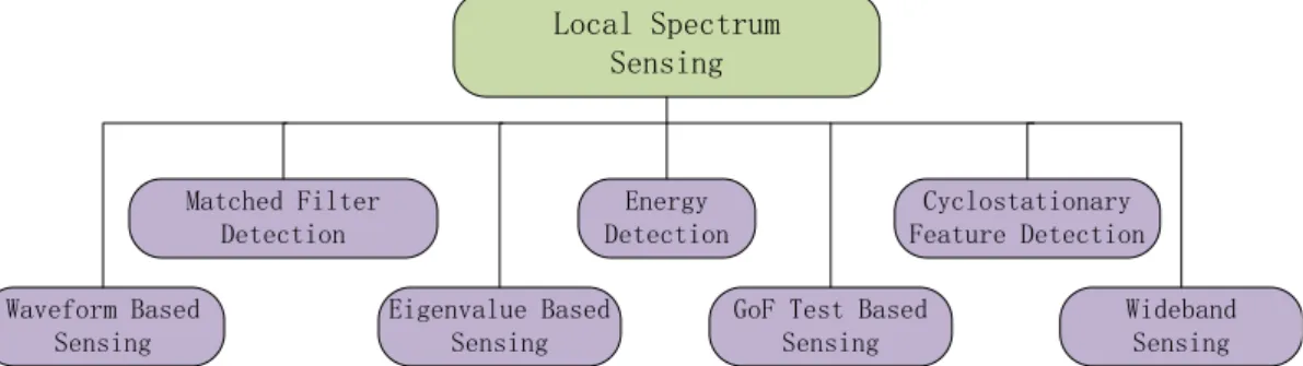
Most common local spectrum sensing techniques, which are listed in Figure 2.3,

will be briefly explained in the next sections.

Cyclostationary Feature Detection Local Spectrum Sensing Energy Detection Matched Filter Detection Eigenvalue Based Sensing Waveform Based Sensing Wideband Sensing GoF Test Based

Sensing

(33)

2.2.1 Matched filter detection

The matched filter detection, which is a traditional coherent signal detection method, is known as the optimum method when transmitted signal is known at the receiver side [34]. Based on the signal model in (2.1), assume that y[n] is the input to a finite impulse response (FIR) filter with impulse response h[n], where h[n] is nonzero for

n = 0, 1,_{· · · , N}s 1, then the output at time n is

Output[n] =

n

X

k=0

h[n k]y[n]. (2.6)

Let the impulse response be a “flipped around” version of the signal s[n] with

power 2 s or h[n] = s[Ns 1 n] n = 0, 1,· · · , Ns 1 (2.7) then Output[n] = n X k=1 s[Ns 1 (n k)]y[k]. (2.8) MFD MFD [ ] y n 1 0 MFD [ ] h n [ 1 ] 0,1, , 1 [ ] 0 otherwise s s s N n n N h n FIR filter 1 s n N BPF ( ) y t ADC

Figure 2.4 – Block diagram of matched filter detection [19].

Define the test statistic of the matched filter detection as the output at time n =

Ns 1, which is given by [19]

TM F D =Output[Ns 1] = NXs 1

k=0

s[k]y[k]. (2.9)

By comparing this test statistic with a threshold ⇣M F D, a decision whether the PU

(34)

The block diagram of matched filter detection is illustrated in Figure2.4. As shown

in Figure2.4, the received signal y(t) goes through a band pass filter (BPF) to reject

out of band noise and adjacent signals, and then Nyquist sampling analogy-to-digital

converter (ADC), a FIR filter are applied to get the test statistic TM F D.

The test statistic TM F Dis proved to be Gaussian under either hypothesis [29]. Thus

TM F D ⇠ 8 > < > : N (0, 2 w"), H0 N (", w2"), H1 (2.10)

where N presents a Gaussian distribution and " =NPs 1

n=0

s2_[n].

Then Pdand Pf a can be evaluated as:

Pd= Q " p " 2 w (2.11) and Pf a = Q p " 2 w , (2.12)

respectively, where is the SNR at SU and Q(x) =R_x1e v2_/2

dv/p2⇡.

The main advantage of this method is that it maximizes the output SNR for a given signal and needs less detection time because it requires only O(1/SNR) sample to meet a given probability of detection constraint [62]. The minimum number of samples is a

function of the SNR = 2

s/ w2, given by [29]

Ns= Q 1(Pf a) Q 1(Pd)

2 ₁

(2.13)

However, in order to get high processing gain and less detection time, this method needs perfect knowledge of PU’s signal feature such as bandwidth, modulation type, etc.. And as a coherent detection method, it requires synchronization with PU, which is an unreasonable assumption in most typical spectrum sensing scenarios. In addition, due to various signal types, the implementation complexity of sensing unit is high.

(35)

2.2.2 Cyclostationary feature detection

The cyclostationary feature detection is an effective detection method which is

implemented based on the cyclostationary property of the received signal [63, 64,65,

66, 67, 68]. In general, modulated signals are coupled with sine wave carriers, cyclic prefixes, etc., which result in built-in periodicity. Therefore, they can be characterized as cyclostationary. Since the noise is wide-sense stationary with no correlation, the cyclostationary feature based detection can be used for detecting the presence of PU signal. Furthermore, cyclostationary feature can be used for distinguishing among different types of transmissions and PUs [67].

For a cyclostationary process s[n], its mean and autocorrelation are periodic in

time. Thus, its cyclic autocorrelation function (CAF) R↵

ss[k] = E s[n]s⇤[n k]e j2⇡↵n

and conjugate cyclic autocorrelation function (CCAF) R↵

ss⇤[k] = E s[n]s[n k]e j2⇡↵n

are nonzero for a set of cyclic frequencies ↵ (↵ 6= 0); on the other hand, for a signal which does not exhibit cyclostationarity, i.e. white Gaussian noise, its CAF

R↵

ww[k] = 0 and CCAF R↵ww⇤[k] = 0, 8↵ 6= 0. Therefore, according to the signal

model in Equation (2.1), an estimation of the conjugate cyclic autocorrelation function

of the observation samples at cyclic frequency ↵ may be obtained using Ns

observa-tions as [67]: ˆ R↵_yy⇤[k] = 1 Ns Ns X n=1 y[n]y⇤[n + k]e j2⇡↵n (2.14) = R↵_yy⇤[k] + "↵_yy⇤[k] (2.15)

where k is the lag parameter in the autocorrelation and "↵

yy⇤[k]is the estimation error

which vanishes asymptotically as Ns ! 1. In practice, due to the error "↵yy⇤[k], the

estimation ˆR↵

yy⇤[k] is seldom exactly zero and a decision has to be made whether a

given value of ˆR↵

yy⇤[k]presents a zero or not [64].

In general, a vector of ˆR↵

yy⇤[k] rather than a value is considered in order to check

simultaneously for the presence of cycles in a set of lags k.

Let k1, k2,· · · , kN be a fixed set of lags, ↵ be a candidate cycle-frequency, A

de-note the set of cyclic frequencies of interest, and

ˆr↵_yy⇤ = h Re Rˆ↵yy⇤[k1] ,· · · , Re Rˆ↵yy⇤[kN] , Im Rˆ↵yy⇤[k1] ,· · · , Im Rˆ↵yy⇤[kN] i (2.16)

(36)

denote a 1 ⇥ 2N vector consisting of the estimated cyclic autocorrelations from (2.14)

with Re and Im representing the real and imaginary parts, respectively. If the

asymptotic (true) value of ˆr↵

yy⇤ is given as r↵_yy⇤ r↵_yy⇤ = h Re R↵yy⇤[k1] ,· · · , Re R↵yy⇤[kN] , Im R↵yy⇤[k1] ,· · · , Im R↵yy⇤[kN] i , (2.17)

then the estimation in Equation (2.15) becomes

ˆr↵_yy⇤ = r↵yy⇤+ "↵yy⇤, (2.18) where "↵_yy⇤ = h Re "↵yy⇤[k1] ,· · · , Re "↵yy⇤[kN] , Im "↵yy⇤[k1] ,· · · , Im "↵yy⇤[kN] i . (2.19)

Finally, by finding out whether there exists cyclic components in ˆr↵

yy⇤, the

hypoth-esis test in Equation (2.1) is reformulated in the following:

H0 : 8↵ 2 A, 8{kn}Nn=1 =) ˆr↵yy⇤ = "↵yy⇤

H1 : ↵2 A, for some{kn}Nn=1 =) ˆryy↵⇤ = r↵_yy⇤ + "↵_yy⇤.

(2.20)

The test statistic relying on the estimation ˆr↵

yy⇤ is given by [64] TCF D = Nsˆr↵yy⇤Pˆ 1 2c(ˆr ↵ yy⇤)T (2.21)

where ˆP_2cis the covariance matrix of ˆr↵

yy⇤, whose computation is given in Appendix

A. Under the null hypothesis H0, TCF D is asymptotically 22N-distributed. Thus, the

probability of false alarm Pf a is derived:

Pf a = P (TCF D > ⇣CF D|H0) = 1 F 2

2N(⇣CF D), (2.22)

where F 2

2N is the cumulative distribution function of

2

2N-distribution and ⇣CF D is a

(37)

Analysis of cyclic Correlation CFD CFD [ ] y n 1 0 CFD BPF ( ) y t ADC

Figure 2.5 – Block diagram of cyclostationary feature detection.

for Nslarge enough approximate a Gaussian distribution [64], as follows

TCF D ⇠ N (Nsr↵yy⇤P_2c1(r↵_yy⇤)T, 4Nsr↵yy⇤P_2c1(r↵_yy⇤)T). (2.23)

Therefore, after getting the threshold ⇣CF D by Equation (2.22), the probability of

de-tection Pdcan be evaluated by

Pd = P (TCF D > ⇣CF D|H1) = Q

⇣⇣CF D Nsr↵yy⇤P_2c1(r↵_yy⇤)T

4Nsr↵yy⇤P_2c1(r↵_yy⇤)T

⌘

. (2.24)

The block diagram of cyclostationary feature detection is illustrated in Figure2.5.

There are various implementations of cyclostationary feature detector in the litera-ture. In [32], two detectors based on estimating the spectral correlation density and the magnitude squared coherence are proposed, which present a good performance in the low SNR. In addition, a hardware implementation of a cyclostationary feature detector is presented in [68], where a detection of 802.11g wireless regional access network (WLAN) signal from air is demonstrated by the cyclostationary feature detector. How-ever, this method also requires a prior knowledge of the signal characteristics, and it needs a long observation time and complex computation.

2.2.3 Energy detection

Energy detection, which is a non-coherent detection method, has been demon-strated to be simple, blind and able to detect the PU signal based on the received

energy. A block diagram of ED is shown in Figure2.6.

In Figure 2.6, the received signal y(t) goes through a BPF to reject out of band

noise and adjacent signals, and then Nyquist sampling ADC, square-law device and

(38)

ED ED [ ] y n 1 0 ED BPF ( ) y t ADC 2 1 | [ ] | s N n y n

Figure 2.6 – Block diagram of energy detection.

As shown in the following equation:

TED =

Ns

X

n=1

|y[n]|2 _(2.25)

where y[n] is the n-th sample of the received signal and Nsis the length of the sample.

In order to more comprehensively understand the performance of energy detection, two analyses of ED including exact performance and Gaussian approximation (GA) are considered as follows.

• Exact performance

The test statistic TED in Equation (2.25) has been proven to follow a central

chi-square ( 2_{) distribution with N}

sdegrees of freedom when there is no signal

transmission from PU. Otherwise, it follows a noncentral 2_{distribution with N}

s

degrees of freedom and a non centrality parameter Ns [37,69]. Following the

short-hand notations mentioned at the beginning of Section2.1, the test statistic

can be described as TED ⇠ 8 > < > : 2 Ns, H0 2 Ns(Ns ), H1 (2.26) where is the SNR of PU signal at SU.

(39)

by [70,71] Pd= P (TED > ⇣ED|H1) = 1 F 2 Ns ✓ 2⇣ED 2 x+ 2w ◆ (2.27) Pf a = P (TED > ⇣ED|H0) = 1 F 2 Ns ✓ 2⇣ED 2 w ◆ (2.28)

where ⇣ED is a predetermined threshold, F 2

Ns presents the cumulative

distribu-tion funcdistribu-tion (CDF) of 2 _{distribution with N}

s degrees of freedom, 2x and w2

denotes the variance of x[n] and w[n].

According to Equations (2.27) and (2.28), by eliminating the threshold ⇣ED, the

ROC can be obtained as

Pd = 1 F 2 Ns 0 @F 1 2 Ns(1 Pf a) 1 + x2 2 w 1 A (2.29) where x2 2 w = is the SNR and F 1 2

Ns is the inverse function F

2 Ns.

In the exact performance analysis, in order to achieve a prescribed performance

(Pf a, Pd) for a given SNR , the minimum number of samples Ns needs to be

exactly calculated. Because Ns can not be obtained from Equation (2.29), it is

necessary to execute multiple evaluations of two-dimensional functions such as

F 2

N and F

1

2

N, which has a huge computational complexity in exact

2

distribu-tion performance analysis [13].

• Gaussian approximation

In order to use low-complexity analytical expressions about the required number

of samples, it has been extensively shown that the test statistics TED can be well

approximated as a Gaussian distribution N . This is because the central limit theorem conditions are satisfied by the large number of the received samples

(e.g. Ns >200). As a result, the following expressions are obtained.

TED ⇠ 8 > < > : N (Ns, 2Ns), H0 N (Ns( + 1), 2Ns(2 + 1)), H1 (2.30)

(40)

Then, in this case, the performance indicators Pdand Pf acan be written as Pd= 1 p 2⇡ 1 Z 1 ⇣ED exp⇣ (t µ1)2 2 2 1 ⌘ dt (2.31) = Q ⇣ED µ1 1 (2.32) and Pf a = 1 p 2⇡ 0 Z ₁ ⇣ED exp⇣ (t µ0)2 2 2 0 ⌘ dt (2.33) = Q ⇣ED µ0 0 , (2.34)

respectively, where µ0 = Ns, µ1 = Ns( + 1)and 20 = 2Ns, 12 = 2Ns(2 + 1)

are the means and variances of the Gaussian distribution in Equation (2.30) under

both hypotheses H0 and H1. Combining Equations (2.30), (2.32) and (2.34),

Equation (2.29) becomes Pd= Q ⇣ (1 + ) 1Q 1(Pf a) (1 + ) 1 p Ns ⌘ (2.35) where Q(x) =R_x1e v2_/2

dv/p2⇡and Q 1_{is the inverse function of Q. Clearly,}

for a fixed Pf a in Equation (2.35), with the increasing of the samples Ns, the

probability of detection Pd rises up at any SNR. That is to say, if the sensing

time is arbitrarily long, Pd ! 1. However, in practice, this is typically not the

case.

The Figure2.7 shows the ROC comparison of ED for the exact 2 _{model and the}

Gaussian approximation model when the SNR = -5 dB. As shown, the classical

GA in Equation (2.35) significantly deviates from the exact result in Equation (2.29).

Conversely, with the increase of the number of samples from Ns = 10to Ns= 100, the

deviated distance is clearly reduced. This also verifies that the Gaussian approximation

of ED is a good estimation only when the number of samples Nsis sufficiently high.

In addition, the effect of the uncertainty of noise power is also a disadvantage of ED. In ED, a decision whether the PU signal exists or not is simply made by comparing

the statistic TED with the noise power. Thus, accurate knowledge of the noise power

is necessary to get a reliable detection performance. However, in practice, the noise

uncertainty is always present. Assume that the estimated noise power is ˆ2

(41)

Probability of false alarm 0.1 0.2 0.3 0.4 0.5 0.6 0.7 0.8 0.9 1 Probability of detection 0.1 0.2 0.3 0.4 0.5 0.6 0.7 0.8 0.9 1 Exact GA N_s=100 N_s=35 N_s=10

Figure 2.7 – The ROC comparison of ED for the exact chi-squared model and the Gaussian approximation model.

(42)

where is called the noise uncertainty factor. The bound of the noise uncertainty (in dB) is defined as [72]

B = sup {10log10 } . (2.36)

And (in dB) is evenly distributed in an interval [ B, B]. When the noise uncertainty exists, ED is not a reliable sensing method [73]. However, ED still becomes one of the most popular sensing techniques in cooperative spectrum sensing because of its simple operations and no requirement on a prior knowledge of PU signals.

2.2.4 Waveform based sensing

Waveform-based sensing (WBS) aims to detect a prior known signals or sequences

expected with the PU signal through correlation detection [21, 40,41,42], which is a

simplified version of the matched filter detection where the exact PU signal is required. Many wireless systems introduce known pre-patterns such as preambles, transmitted pilot patterns, spreading sequences, etc. to assist synchronization or for other purposes. Correlation between the received signal and a known copy of itself can be used to detect the presence of a PU signal exhibiting this pattern. As shown in [40], waveform-based sensing has better detection performance and requires shorter sensing time over the energy detection. However, WBS needs to assume that a pattern exists in the PU signal, and SU must know and detect this information. Especially when a wide range of PU needs to be detected, the database of known pattern for SU may become large and complex to manage. Moreover, synchronisation is required between PU and SU and an error of synchronization can severely degrade the detection performance. Comparing with the matched filter detection, waveform based sensing has a lower complexity [21].

2.2.5 Eigenvalue based sensing

As a result of requiring no prior information of the PU signal or no noise variance, eigenvalue based detection has been widely investigated for blind spectrum sensing

methods in CR [43,44,45, 46, 47,48,49,50]. Those eigenvalue based methods

usu-ally utilize the correlation structure inherent in the received data for sensing, which results from the multipath propagation and/or oversampling of the PUs signal for a single-antenna receiver or the deterministic channel during the sensing period for a multiantenna receiver. It also involves that the statistical covariance matrices or the eigenvalues of the covariance matrix of signal and noise are different. Thus, the

(43)

dif-ference is used to differentiate the signal component from background noise in those eigenvalue based methods where the knowledge of the noise variance is not required.

Considering L (called “smoothing factor”) consecutive samples and defining the following vectors:

ydef=⇥y[n] y[n 1] y[n 2] . . . y[n L + 1]⇤T (2.37)

xdef=⇥x[n] x[n 1] x[n 2] . . . x[n L + 1]⇤T (2.38)

wdef=⇥w[n] w[n 1] w[n 2] . . . w[n L + 1]⇤T. (2.39)

We can define the statistical covariance matrices of the received signal, the trans-mitted signal passing through a wireless channel and the corresponding noise as

Ry =E ⇥ yyH⇤, (2.40) Rx =E ⇥ xxH⇤, (2.41) Rw =E ⇥ wwH⇤. (2.42)

where (·)H _{denotes the conjugate transpose and E[·] is the mathematical expectation.}

According to Equations (2.37-2.42), the hypothesis test in Equation (2.1) can be

reformulated as follows:

H0 :Ry =Rw

H1 :Ry =Rx+Rw,

(2.43)

In practice, a finite number of samples can be obtained for calculating the statistical covariance matrix. Define the sample auto-correlations of the received signal as

(k) = lim Ns!1 1 Ns NXs 1 n=0 y[n]y[n k], k = 0, 1, . . . , L 1. (2.44)

where Ns is the number of collected samples.

(44)

covari-ance matrix defined as Ry(Ns) = 2 6 6 6 6 4 (0) (1) · · · (L 1) (1) (0) · · · (L 2) ... ... ... ... (L 1) (L 2) _{· · ·} (0) 3 7 7 7 7 5 (2.45)

where the sample covariance matrix is a Toeplitz matrix, and it is also symmetric. The

eigenvalues ofRy(Ns)are defined as 1 2 . . . L.

Depending on the difference of the statistical covariance matrices or its eigenvalue between signal and noise, several covariance matrix or eigenvalue based methods have been proposed in literature [50], such as the maximum-minimum eigenvalue (MME) method [14], the eigenvalue arithmetic-to-geometric mean (AGM) method [15], the covariance absolute value (CAV) method [16], the scaled largest eigenvalue (SLE) method [17] and the function of matrix based detection (FMD) method [18]. These methods will be explained in the following.

• Maximum-minimum eigenvalue (MME) method:

The MME method firstly takes advantage of the ratio of the maximum over the

minimum eigenvalue of the sample covariance matrix, that is, max/ min, in

order to decide that the PU signal is present or not. The test statistic of the MME method is given by [14] TM M E = max min H1 ? H0 ⇣M M E, (2.46)

where ⇣M M E is the decision threshold. If max/ min > ⇣M M E, the signal exists;

otherwise, the signal does not exist. The MME method overcomes the noise uncertainty problem and can even perform better than the energy detection when the samples of the signal to be detected are highly correlated.

• Arithmetic-to-geometric mean (AGM) method:

The AGM method is derived from a generalized likelihood ratio test (GLRT),

which only depends on the observations through ˆRy(Ns). The test statistic is

(45)

eigen-values of the sample covariance matrix, which is given by [15] TAGM = 1 L L P i=1 i ( L Q i=1 i) 1 L H1 ? H0 ⇣AGM (2.47)

where 1 2 . . . Lare the decreasing sampling eigenvalues of ˆRy(Ns)

and ⇣AGM is the decision threshold of the AGM method.

• Covariance absolute value (CAV) method:

The CAV method makes use of the difference of the statistical covariances of

the received signal and noise. When signal is not present, Rx = 0. Hence,

Ry =Rw = 2wIL, its off-diagonal elements are all zeros. When there is a signal

and the signal samples are correlated,Rxis not a diagonal matrix. Hence,Ry =

Rx+ 2wIL, some of its off-diagonal elements should be nonzeros. According to

this, the test statistic of the CAV method is given by [16]

TCAV = T1 T2 H1 ? H0 ⇣CAV (2.48)

where ⇣CAV is the decision threshold of the CAV method, and the two values T1

and T2are calculated by

T1 = 1 L L X i=1 L X j=1 |ri,j| (2.49) T2 = 1 L L X i=1 |ri,i| (2.50)

where ri,j is the (i, j) entry of the sample covariance matrix ˆRy(Ns).

• Scaled largest eigenvalue (SLE) method:

When the number of PUs (or rank) is a priori known, the accurate generalized likelihood ratio (GLR) method is proposed [17]. In the presence of a signal PU, the rank-1 GLR detector employs the SLE as its statistic, which is called the SLE method and is expressed as

TSLE = 1 1 L L P i=1 i H1 ? H0 ⇣SLE (2.51)