Modeling of Thermoplastic Welding

HAL Id: hal-02591944

https://hal.archives-ouvertes.fr/hal-02591944

HAL is a multi-disciplinary open access archive for the deposit and dissemination of sci-entific research documents, whether they are pub-lished or not. The documents may come from teaching and research institutions in France or abroad, or from public or private research centers.

L’archive ouverte pluridisciplinaire HAL, est destinée au dépôt et à la diffusion de documents scientifiques de niveau recherche, publiés ou non, émanant des établissements d’enseignement et de recherche français ou étrangers, des laboratoires publics ou privés.

Modeling of Thermoplastic Welding

Gilles Régnier, Steven Le Corre

To cite this version:

Gilles Régnier, Steven Le Corre. Modeling of Thermoplastic Welding. Nicolas Boyard. Heat Transfer in Polymer Composite Materials : Forming Processes, Wiley, pp.235-268, 2016, 978-111911628-8;978-184821761-4. �10.1002/9781119116288.ch8�. �hal-02591944�

Modeling of thermoplastic welding

Gilles Régnier

, Steven Le Corre

1 : PIMM, Arts et Métiers ParisTech, CNRS, CNAM 151 bd de l’Hôpital, 75013 PARIS (France) 2 : Laboratoire de thermocinétique, Polytech Nantes, CNRS

La Chantrerie, Rue Christian Pauc, BP 90604, 44306 Nantes Cedex 3 (France)

Abstract

Welding of thermoplastic materials or thermoplastic composite parts is a valuable process as it allows designing parts with quite simple forms and assembling them without adding material. Nevertheless, the mechanical properties around the welded line are often significantly lower the ones of bulk materials. Optimizing the mechanical properties requires the understanding of the physical mechanisms involved in welding processes. Intimate contact and macromolecular diffusion, which are the two main physical phenomena that govern healing of interfaces, are presented in details. As these phenomena depend a lot on temperature and welding processes are highly anisothermal, thermal modellings of processes or accurate local temperature measurements are necessary to record temperature histories around welded lines and to predict interface healing. The welding of thermoplastic composite tapes is modelled for two types of heating: hot nitrogen torches and ultrasounds. We show how the phenomena are coupled in the thermo-physical simulations. Moreover, heating can degrade the polymer, therefore modify the molecular mass and then directly interact with macromolecular diffusion phenomena.

1. Introduction

1.1. Polymer welding processes

Welding is a well-established technology in the thermoplastic industry where the efficiency of welded joints can approach the properties of bulk materials. Thermoplastics or thermoplastic matrix composites can be assembled in such a way by heating them at a temperature above glass transition for amorphous matrix and above fusion temperature for semicrystalline matrix. Thermoplastic welding technologies can be classified according to the technology introducing the type of heating [1,2]. We proposed to classify them into three classes: bulk heating, surface heating and mechanical energy dissipation techniques.

Bulk heating techniques (compression moulding, electromagnetic heating techniques such as microwaves or dielectric welding [3], autoclaving and induction for some composites) are available for performing a joining method with no added weight to the final structure. For multi-layer composites, which are excellent shields in the microwave range [4], microwave welding is poorly suitable especially when composites are reinforced by carbon fibers. Induction heating technique is available if thermoplastics are reinforced by conductive materials (ferromagnetic materials): iron particles, micrometer-sized particles of iron oxide, stainless steel, specific ceramic, ferrite or graphite, acting as susceptors [5]. However, in all cases, the entire part is brought to the melt temperature and a complex tooling is generally needed to maintain pressure on the entire part in order to prevent de-consolidation.

Hot melt thermoplastic adhesive films [6] or amorphous films involving co-molding of an amorphous thermoplastic to a semi-crystalline matrix laminate prior to bonding may also be inserted between the welded surfaces to improve filling of part mismatch [7].

In surface substrate heating techniques (hot plate welding, hot gas welding, radiant welding, laser welding), the heating device should to be removed from the surfaces between the stages of heating and welding, except for resistive implant welding also called electro-fusion welding [8]. Heating times may be long because of the low thermal conduction of polymer matrix. Between heating and welding stages, surface temperature may drop and the region having the maximum temperature is located below the skin of the part [9]. Then, the pressure required to consolidate the joined surface may cause warpage/flow in the higher temperature inner region [10]. As the whole welding surface must be heated rather uniformly, these processes involve limitations on size and geometry of the parts.

Heating by mechanical dissipation techniques (ultrasonic welding, vibration welding, spin welding) have been widely used in the plastics industry [11]. Vibration welding and spin welding are less appropriate to joining thermoplastic composites as the motion of the substrates may cause deterioration or modification of the local microstructure [12]. Ultrasonic welding is certainly one of the most commonly used welding processes for thermoplastics with many applications in automotive parts [11]. To dissipate mechanical energy, small asperities called energy directors generally in the form of triangular protrusions are molded onto the part to initiate melting. Nevertheless, ultrasonic welding applications to flexible polymers or semicrystalline polymers with a rubbery amorphous phase are limited since they absorb most of energy in bulk [10]. Kenney [13] insisted to consider the requirements of ultrasonic welding at the early stage of the design of a part.

1.2. Healing mechanisms of polymer interfaces

For all these welding processes, the healing of the polymer/polymer interface was described by Wool et al. [14] who identified three main sequential stages, namely: (1) surface rearrangement and surface approach; (2) wetting; (3) diffusion. In stage (1), the interface has no mechanical properties as the two distinct faces still exist. The completion of the wetting stage marks the achievement of intimate contact between the two surfaces. Potential barriers associated with inhomogeneities or porosities at the interface have disappeared, and molecular chains are free to move across the interface in a process of inter-diffusion also called autohesion, which leads ultimately to the collapse of the interface.

Wool et al. [14] proposed to model the wetting stage by a phenomenological approach of nucleation and radial growth of wetting surface, which led an expression of Avrami’s type. Nevertheless, the time scale of wetting phenomenon is very difficult to quantify experimentally. It is also difficult to separate this phenomenon from surface rearrangement. As it seems that the time scale of wetting phenomenon is one order of magnitude less than surface rearrangement and molecular diffusion, most of researchers have gather stages (1) and (2) into one stage generally called intimate contact. Modeling of intimate contact and macromolecular diffusion stages are presented in the next section.

2. Physics of thermoplastic welding

2.1 Intimate contact at interface

Whatever the elaboration technique of polymer or composite parts, surfaces always present a certain roughness. Micro-asperities and micro-valleys as well as more macroscopic surface waves lead to a non-perfect contact between the two parts to assemble. As commonly admitted in thermoplastic welding, intimate contact is the first step in forming a bond between two thermoplastic surfaces that have been brought together under both heat and pressure [15, 16, 17]. As visible from Figure 1, surface roughness may be very important, leading to a rather low initial area of contact between the two adjacent surfaces.

Figure 1- Cross section of an APC2 Carbon/PEEK composite tape (a) and associated roughness profile (b) [18].

The quality of the contact can be described through the concept of degree of intimate contact Dic, as introduced by Lee and Springer [19]. It is a macroscopic descriptor of the contact that can be defined as the ratio of the real contact area Acont to the total area of the surfaces to be welded Atot:

𝐷𝑖𝑖 = 𝐴_𝐴𝑐𝑐𝑐𝑐

𝑐𝑐𝑐

Eq. (1) In thermal studies, it is known as the real rate of contact. To describe this variable, one may use optical profilometers that nowadays enable to characterize solid surfaces from nanometric to millimetric scales. They easily provide statistic descriptors such as the arithmetic roughness Ra, the quadratic one Rm, or the average slope of the profile. Automated devices are also able to produce full surface reconstructions, suited for finer modeling [20].

Once the surface topography is obtained, the main problem is the prediction of its evolution while submitted to the welding pressure. This question has been the subject of several models during the last couple of decades. Dara and Loos [21] developed a model representing the surface of a thermoplastic as a distribution of rectangles of different size. Lee and Springer [19] simplified this model by using rectangular elements of the same size (Figure 1). Their approach, owing to its great simplicity and efficiency, has now become the most widely used. In the representation of Figure 2, the degree of intimate contact can be defined as:

𝐷𝑖𝑖 = _𝑏 𝑏 0+𝑤0

Eq. (2) where the geometrical parameters b, b0 and w0 are defined in Figure 2a. In this very idealized

picture, the surface topography is described by its average roughness, that may be finally attributed to the height a of rectangles, as proposed in [22,23,24].

Figure 2 – (a) Idealization of surface asperities by periodic rectangular elements, before and after squeezing

[19], (b) Fractal Cantor set description of the adherents surface [18]. Then using the volume conservation of rectangles, one can write:

𝐷𝑖𝑖 = _1+𝑤𝑎/𝑎_0/𝑏0 ₀ Eq. (3)

The squeezing kinematics is then modeled by a so-called “squeeze flow” model for a Newtonian fluid, and leads to the following differential form [22]:

𝐷̇𝑖𝑖 = �𝐷_𝐷𝑖𝑐,0_𝑖𝑐� 4 �𝑎0 𝑏0� 2 _𝑃 𝜇�𝑇(𝑡)� Eq. (4) where 𝑃 is the applied pressure and where the viscosity of the thermoplastic 𝜇 can be defined by an Arrhenius type law. It reduces to the Lee & Springer’s model in an isothermal case:

𝐷𝑖𝑖 = _1+𝑤1_0/𝑏0 �1 +_𝜇(𝑇)5𝑃 �1 +𝑤_𝑏00� �𝑎_𝑏00� 2

𝑡� Eq. (5)

Those expressions clearly underline the role of time, pressure and temperature - through its direct influence on the viscosity - as well as thermoplastic initial surface quality, through rudimental parameters a0, b0 and w0 [15, 24, 25].

In order to improve such a rough description of the surface profile, the fractal Cantor set based model was proposed by Yang and Pitchumani [23, 25]. Parameters a0, b0 and w0 cannot be determined physically and must therefore be fitted using experimental results. Their approach consists in describing the surface morphology as a Cantor set fractal surface (Figure 2b), where each geometric parameter can be obtained from a surface profile measurement. The squeezing kinetics of this morphology and the resulting evolution of Dic is then calculated by the Lee and Springer rectangular model [19], applied iteratively from the smallest to the biggest rectangles of the fractal geometry [23]. As illustrated in the parametric study of Figure 3, the model is sensitive the fractal dimension D and capable of predicting more subtle effect than the idealized rectangle approach. One of the main benefits of this method is that it can be based on direct surface measurements as illustrated in several implementations [23, 24, 26, 27, 28]. As the fractal Cantor model is scale-invariant, the precise accuracy of a particular measuring method is not of significant importance [28].

More recently a model using a more realistic description of the initial surface has been proposed [20]. The surface geometry was measured by a profilometer and meshed. The squeezing step was hen computed using Polyflow® software. The authors showed a good correlation of this new model with the Lee and Springer model.

Figure 3: Parametric effects of the fractal surface parameters on the development of the Dic contact [23].

Despite the different attempts of reaching a finer geometrical description of surface roughness, the simple idealized rectangle model still seems to remain the most simple and efficient as the numerous successful applications of it show [2,22,29,30,31,32]. Nevertheless, the underlying assumptions of this approach are very restrictive (2D model, Newtonian squeeze flow) and further improvements are expected in the future, especially for an optimal control of interlaminar adhesion of thermoplastic composite parts. Furthermore, experimental measurements of the Dic during processing, which are generally assumed impossible, can be done through thermal measurements [18]. Finer validations of those intimate contact models should also be possible.

2.2. Macromolecular diffusion 2.2.1. Modeling of a polymer chain

At equilibrium in a melted state, a polymer chain takes the configuration of a statistical pellet [33] with a given gyration radius Rg and a chain end-to-end distance R. Many authors [33-35] have modeled this statistical pellet as a set of n freely jointed rigid segments having a length l (Figure 4), therefore the length of the stretched chain is equal to nl. It is shown that the mean square values of gyration radius Rg and chain end-to-end distance R are:

〈𝑅2_{〉 = 𝑛𝑙}2 _{and 〈𝑅}

𝑔2〉 = 〈𝑅2〉/6 Eq. (6)

In a real polymer chain, the segments are not fully free in all directions, then <R2> and <Rg2> increase. Flory defined [33] the chain characteristic ratio C_∞as the ratio of the real polymer mean-square end-to-end distance <R2>0 and that of a freely jointed chain:

Eq. (7) The chain appears to be more flexible when C_∞decreases. Values of C_∞are given for some polymers [35]: C_∞is equal to 8.26 for PE and to 6.15 for iPP.

Another way to express the fact that chain segments are not fully free in all directions is to consider the Kuhn length defined as the effective monomer size for the equivalent freely jointed chain (N Kuhn monomers of length b). The length of the considered chain is equal to

nl=Nb. The real polymer mean-square end-to-end distance <R2>0 is then equal to: 2 0 2 R C nl ∞ < > =

Eq. (8) From Eq.(8), it can be deduced that b=C l_∞

Figure 4 - Freely-jointed segment model 2.2.2. Modeling of macromolecular diffusion

A large amount of works exists on the study of polymer chain movements, most of them are based on the previous chain modeling. Only the most significant for the topic are presented. Rouse [36] proposed to model the polymer chain by a set of beads freely-joined by springs. He showed that the time τ_Rouseneeded to have an overall movement of the chain is equal to:

Eq. (9) where ξ is a friction coefficient, kb the Boltzmann constant, b and N Kuhn parameters and T the temperature. This Rouse time is proportional to the square of the chain length or the molecular mass. It turns out that this model applies quite well for polymer chains or chain branches having a molecular mass less than the critical molecular mass Mc, which denotes the transition in the melt viscosity versus molecular mass relation as the exponent changes from 1 to 3.4. The ratio of Mc to molecular mass between entanglements Me has long taken to be 2 and thus independently to species. However, an empirical compilation [37] has shown that this ratio varies from 1.4 to 3.5.

For polymer chains having a molecular mass larger than Mc, ie for entangled polymer chains, molecular movements can be divided in two types:

- Movements at a small scale which do not affect the topology of entanglements. The scale time of these movement is Rouse time.

- Movements at a larger scale which modify the topology of entanglements. These movements obey to another scale time because chains interact with neighboring.

For the last type of molecular movement, de Gennes [38] proposed the well-accepted reptation theory in which the polymer chain is confined in a tube, which is supposed to model the constraints of neighboring chains. The chain has a Brownian movement and can only exit the tube by its two extremities. The tube disappears and appears gradually (Figure 5) as the chain moves as a snake in the tube, hence the reptation theory. The time required for the chain to completely exit the initial tube and then to totally loose the memory of its initial configuration is: Eq. (10) 2 2 2 0 R C nl_∞ Nb < > = = Rg R l 2 3 ² Rouse B bN k T ξ τ π = 4 3 3 3 ² Reptation B b N k Ta ξ τ π =

where a is the diameter of the tube, which can be approximated to the mean square distance between entanglements:

Eq. (11) with Ne equal to the number of Kuhn segments between entanglements. Therefore, the reptation time is proportional to the cube of chain length or molecular mass. Then, the ratio between reptation time and Rouse time is:

Eq. (12) For example, the ratio between reptation time and Rouse time is nearly two decades for an injection molding PE with a molecular mass of 60 kg/mol, knowing that the mass between entanglements for PE is equal to 1.4 kg/mol [35].

Figure 5 – Reptation theory of de Gennes 2.2.3 Macromolecular diffusion and polymer interface healing Amorphous polymers

Numerous theoretical and experimental studies have been done on interface healing of amorphous polymers. Most of them are based on chain reptation mechanism. De Gennes [39] considered that healing is driven by the density of chain bridges at the interface, Kausch [40] supposed that healing is related to the number of entanglements formed at the interface and Wool [41] who has most certainly worked on this topic, assessed that healing is controlled by the length of chain interpenetration. All of them found that the ratio of fracture toughness for a healing time t less than the reptation time GIC(t) to the polymer bulk fracture toughness GIC∞

is proportional to the ratio of time t to reptation time at the power 0.5:

Eq. (13) Then, the induced stress necessary to fracture the interface σ(t) varies as:

Eq. (14) Nevertheless, the dependence of stress and fracture toughness with molecular mass varies with modeling and rupture mode. Firstly, it was observed that the bulk fracture toughness is reached for a reptation time corresponding to a polymer of 8Mc and becomes independent of molecular mass [42]. In that case, the fracture mechanism is chain rupture and agrees with scaling laws of de Gennes and Kausch [39-40]:

Eq. (15) 2 2 / 6 e a =b N 2 2 Reptation Rouse e e N M N M τ τ = = 1 2 ( ) IC IC Reptation G t t G _∞ τ   ∝ _ _   1 4 ( ) Reptation t t σ σ_∞ τ   ∝ _ _   1 3 2 2 ( ) IC IC

For PE, 8Mc corresponds to a molecular mass of 40 kg/mol. Yang and Pitchumani [43] supposed it is sufficient that the chains come out of the tube along a distance corresponding to 8Mc to have a good healing.

For a polymer with a molecular mass between Mc and 8Mc, the fracture mechanism should be chain pull out mechanism (disentanglement) and Wool modeling [42] seems to agree with experimental tests:

Eq. (16)

Eq. (17)

Semi-crystalline polymers

In semicrystalline polymers, crystallites constituted of chains from each side of the interface can be formed through the interface during the cooling [44]. This co-crystallization phenomenon occurs with incomplete chain diffusion at the interface and takes part in interface consolidation [17,45,46]. Rupture mechanisms at interface in semicrystalline polymers are therefore more complex and certainly need further investigations to precisely model them. When the amorphous phase in a semicrystalline polymer is glassy at test temperature, rupture mechanisms are probably close to the ones occurring in amorphous polymers having a molecular mass higher than 8Mc, i.e. by chain rupture.

For semicrystalline polymers with rubbery amorphous phase (like PE or PP at ambient temperature), the high mobility of the amorphous phase favors chain pull out and disentanglement. In that case, Fayolle et al. [47] showed that the chain pull out phenomenon occurs for semicrystalline polymers having a molar mass until 50Mc.

3. Linear viscoelasticity to quantify the macromolecular diffusion

Linear viscoelasticity (LVE) precisely reflects the distribution of relaxation times in a polymer and is therefore strongly correlated to the molecular structure, i.e. the molecular weight, molecular weight distribution and molecular architecture [48,49]. Hence, LVE is a powerful tool, which provides fundamental insights about the link between dynamics and polymer structure [50].

From linear viscoelastic frequency sweep tests, two characteristic relaxation times can be determined from the terminal relaxation zone. Firstly the number-average relaxation time

determined as 0

0/

n GN

τ =η can be experimentally obtained from the intersection of the G’’ terminal regime with 0

N

G , where 0

N

G is the plateau modulus and η0 the zero-shear viscosity.

Secondly, the intersection frequency ww of G’ and G’’ terminal regimes gives the weight-average terminal relaxation time τw as follows: τw=1 /ww=Je0η0, where

0

e

J is the steady-state recoverable shear compliance. Therefore, the breadth of relaxation time distribution can be

assessed to 0

0 /

w n Je

τ τ = η and varies in the typical range 2 to 3 for nearly monodisperse polymers or polymers with a very narrow molecular mass distribution [49].

For monodisperse polymers, the reptation time τR of tube models is closely linked to the

terminal peak position of G” [51] and should be intermediate between τw and τn_. No simple

1 1 1 3 2 2 ( ) 2 2 ( ) IC IC IC IC G t G t t M and G M or t M G − − ∞ ∞ ∝ ∝ ∝ 1 1 1 1 3 4 4 2 ( ) 4 4 ( )t t M and M or σ t t M σ σ σ − − ∞ ∞ ∝ ∝ ∝

response can be given for polydisperse polymers as obstacles in tube modeling are not really fixed due to smaller chains.

It is convenient to model the linear viscoelastic response of a polymer by rheological models. The simplest one is certainly the Maxwell model, which has only one relaxation time. Then all relaxation times that can be determined from a frequency sweep response are identical: τ_w,

n τ

, maximum of G”, G’ and G” crossing, viscosity passage from Newtonian to rheothinning

regimes (Figure 6). Thus, this model cannot precisely model the linear viscoelastic response of a monodisperse polymer since τ τ_w/ _n  . But a multimode Maxwell model can either fit 2 the linear viscoelastic response of a monodisperse or a polydisperse polymer, depending on the number of parallel branches.

Figure 6 – Frequency sweep response of a Maxwell multimode model

Relaxation times (0.03/0.1/0.3/1/3/10 s) – Respective associated moduli (100/300/300/300/300/200 MPa)

The question is: which relaxation time should be considered to have a healed interface? Let us first consider an amorphous polymer. For a commercial polymer, ie a polydisperse polymer, the answer is not simple in a general case because molecular movements are complex and it is not so easy to link dynamics and complex polymer structure. In all cases, interface healing surely needs complete polymer chain reorganization, then long relaxation times of the terminal behavior should be considered and τ_wis without any doubt a good assessment of a complete polymer diffusion though the interface.

For semicrystalline polymers, the response is still more complicated because of co-crystallization through interface. Although co-crystallation could improve interface healing, it is safer to consider that interface is healed when the chain diffusion process through the interface is achieved like for amorphous polymers.

For amorphous and semicrystalline thermoplastics, the determination of the terminal relaxation time is often not so easy because wide frequency range master curves should be determined for highly polydisperse polymers. Zanetto [52] and Régnier et al. [53] considered the frequency viscosity passage from Newtonian to rheothinning regimes. Nevertheless, they verified that this relaxation time was not too far from τ_w for one temperature, this was certainly true because the molecular mass distribution of respectively PA12 and PEEK was not too large, which is generally not the case for polyolefins.

4. Application to continuous welding of composite tape

4.1 Process description

Continuous carbon fiber-reinforced tapes are used in the aircraft industry to build structural parts by welding them one to another to constitute the desired part. A two-steps procedure was needed in the past: first a manual or automated tape placement, then a consolidation in autoclave. The aim of this study was to investigate a new process, named “Drapcocot” [54], developed by EADS, Dassault Aviation and Eurocopter, in which placement and consolidation are performed simultaneously in order to increase the productivity.

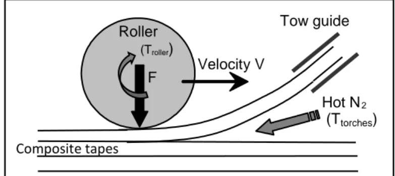
The process principle can be briefly described as follows (Figure 7): the first layers are supposed to be already laid down. Then the tape under consideration is placed in its position using the tow guide. Two torches blow hot nitrogen in order to melt the material at the interface between the plies to weld. A roller applies a normal force on the tape in order to improve the adhesion between the plies. The process parameters that can be controlled are: torches temperature, head velocity, roller temperature and roller force.

The material was the well-known APC-2, pre-impregnated UD carbon-PEEK composite supplied by Cytec.

Figure 7 - Schematic principle of “Drapcocot” process 4.2 Influence of processing conditions on interfacial strength

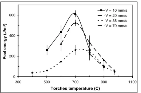
The weld quality was characterized using peel tests on two layers samples, which differed by their processing conditions: torches temperature and lay-down velocity [53]. The applied roller force was kept constant and high enough to make the intimate contact time [30] negligible, compared to the welding time. The peel energy (Figure 8) displays a maximum and it appears thus that adhesion is under the dependence of two antagonist and thermally activated phenomena. The role of velocity puts in evidence the importance of kinetics aspects. In the low temperature torches domain (< 700 C), adhesion is an increasing function of

Composite tapes Roller (Troller) Velocity V

temperature and a decreasing function of velocity, which suggests a thermally activated diffusional process. The decrease of adhesion at high temperature could be explained by thermal ageing, which affects adversely the welding quality. Other phenomena, for instance co-crystallization at interface before complete molecular diffusion may also affect the mechanical performance of welded joints [54].

According to these assumptions, the model elaboration involves three steps: i) Determination of kinetic laws for chain diffusion. ii) Identification of thermal ageing processes susceptible to influence welding and determination of their kinetic parameters. iii) Thermokinetic mapping of the process to determine the material thermal history at every point.

Figure 8 - Influence of parameters on interfacial adhesion 4.3 Modelling of macromolecular diffusion

Once the intimate contact between plies is established, the interdiffusion of macromolecular chains at the interface occurs as long as the matrix is melted, i.e. before crystallization quenches long range chain motions. Unfortunately, the PEEK grade used for APC-2 was not available so that rheometric measurements were made on a pure PEEK grade (Victrex PEEK G450) which was supposed to be the highest boundary of the APC-2 matrix in terms of molecular weight.

As it was difficult to determine experimentally the terminal relaxation time, the diffusion time was assessed by determining the passage between Newtonian and rheothinning domains of complex viscosity η* (see section 3). The measurements were performed on an Ares Rheometric Scientific rheometer using parallel plates geometry under nitrogen in the 310-410 C temperature range at 2% strain amplitude with angular frequency ranging from 0.01 to 100 rad.s-1. It can be recalled that the main temperature transitions of PEEK are glass transition temperature Tg = 140 C, melting point Tm= 330 C and crystallization temperature, which begins at about 280 C in a programmed temperature decreasing experiment.

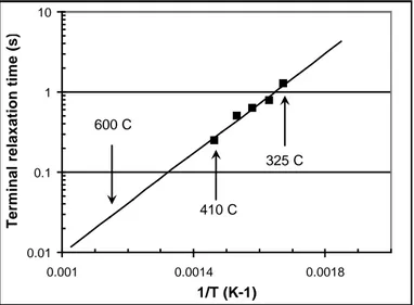
Characteristic relaxation time versus temperature λ(T) (Figure 9) was identified from Carreau law: Eq. (18) 0 200 400 600 300 500 700 900 1100 Torches temperature (C) P ee l e ne rgy ( J/m ²) V = 10 mm/s V = 20 mm/s V = 38 mm/s V = 70 mm/s

(

)

It obeys an Arrhenius law with a consistent activation energy of 59.7 KJ.mol-1 that allows extrapolating it at higher temperatures inaccessible to experiments.

To quantify the extent of reptation in an anisotherm process, it is possible to solve the diffusion equation in the nonisothermal case [14,56]. Yang et al.[43] proposed to consider a diffusion criterion D defined by:

Eq. (19) where D that depends of material thermal history and assessed diffusion time, describes the probability for a chain to cross the interface. D = 1 means that the processing time is equivalent to the reptation time in an isothermal experiment, therefore D has to be larger than 1 to consider the interface healing achieved. D was calculated for various sets of processing parameters taking the origin of time when interfaces are in contact and reach melting point and end of time when crystallization began. For that, a non-isothermal crystallization kinetic was identified and implemented in the model [30]. Thus, it was possible to plot the envelope of points where D = 1 in a process window (see §4.5).

Figure 9 - Variation of Vitrex PEEK G450 relaxation time 4.4 Modelling of thermal aging

According to the literature [57,58] crosslinking is resulting apparently from radical processes and predominates during PEEK thermal ageing under nitrogen. It is expected to disadvantage welding because it increases the melt viscosity. To study crosslinking kinetics, real viscosity η’ was measured in the 360-460 C temperature range at low frequency in order to remain in Newtonian regime. Very small variations were observed, after 6 hours at 360 C, whereas the viscosity increases by almost two orders of magnitude after about 2 hours at 460 C.

Far from the gel point at low conversion, the number of crosslinking events per mass unit Rc varies from initial time (subcript 0) as:

Eq. (20) where Mn and Mw are respectively the number and weight average of molar mass and IP is the polydispersity index.

( )

(

)

dt

D

T t

λ

=

∫

It will be assumed that IP ~ IP0 and viscosity still obeys the power law established for linear chains:

Eq. (21) where K is a temperature dependent material property. More sophisticated relationships taking into account the specific influence of branched architecture in crosslinked polymers on their viscosity are available, but it seems the above equations are sufficient to predict the trend of viscosity variations. Then, the crosslink concentration Rc can be given by:

Eq. (22) Rc was plotted against exposure time in Figure 10a, it varies quasi linearly with time, even at 460 C, in the first hour of exposure.

Figure 10 – (a) Evolution of crosslink concentration Rc with time for different temperatures

(b) Variation of crosslink kinetic rate with temperature

The slope of the linear domain gives the crosslinking kinetic rate Kapp, thus the crosslinking kinetics can be approximated by a zero order process:

Eq. (23) where it appears that the kinetic rate obeys to Arrhenius law (Figure 10b):

Eq. (24) with A = 3384 mol.g-1.s-1 and Ea = 168 kJ.mol-1.

As for diffusion in an anisotherm process, it is possible to define the crosslink concentration Rc representing the extent of thermal ageing in a given point:

Eq. (25) This calculation was implemented in the thermal modelling of the process (next sub-section), then it was possible to plot iso-ageing curves a process window. Peel tests were done on composite tapes consolidated and aged in autoclave for different temperatures. It was found that thermal ageing begins to hinder adhesion for Rc = 10-7 mol.g-1.

3.4 ' KM_w η = 0 0 1/3.4 ' 0 1 ' P c w I R M η η  _{ }    = _{ −   }     0.00000 0.00001 0.00002 0 5000 10000 15000 20000 C ro s s li n k c o n c e n tr a ti o n ( m o l/ g ) Time (s) 360 C 380 C 400 C 420 C 460 C (a) 1.E-11 1.E-10 1.E-09 1.E-08 0.0013 0.0014 0.0015 0.0016 Ka p p (m o l.g -1.s -1) 1/T (K-1₎ (b) c app R =K t exp a app E K A RT   = _− _  

(

)

∫

4.5 Thermal modelling of the process

As thermal conductivity is ten times higher in the fiber direction than in the transverse direction, a time dependent 2D model has been built to predict the evolution of temperature during the process. The 2D model written in Matlab® uses a finite volume formulation with an explicit scheme. The heat transfer from hot nitrogen to the material is characterized by a heat transfer coefficient htorche over a length ltorche before the roller applies the pressure (Figure 11). The interface is considered inexistent in the welded zone so that, thermal exchanges are only due to conduction. The roller imposes a local surface heat flow characterized by its heat transfer coefficient hroller and the contact length lroller.

Figure 11– Principle of thermal modelling

The global heat equation contains two source terms relative to crystallization and melting. Both source terms were identified from DSC characterizations and crystallization kinetic has been implemented to define more precisely the end of macromolecular diffusion process [30]. Small thermocouples inserted between the plies have allowed both model calibration by adjusting the different heat transfer coefficients and temperature evolution validation at temperature measurement locations.

Figure 12 –Velocity-temperature process diagram. The numbers are the ratio P/Preference between process Peel

test values and Peel test reference value obtained for a tape consolidated in autoclave. Arrows show valid domains for diffusion and crosslink concentration criteria.

Air convection Torches convection Welded tapes New tape Roller convection Air convection Air convection 400 600 800 1000 1200 0 10 20 30 40 50 60 70 80 T or c he s te mpe ra tur e (C ) Torches velocity (mm/s) D = 1 0.21 0.36 0.51 0.21 0.26 0.45 0.27 0.13 0.05 0.39 0.21 0.2 0.27 0.39 0.2 0.08 0.04 P / Preference (numbers) D > 1 Rc< 10-7mol/g Rc = 10-7_mol/g

4.6 Weldability prediction

Peel test ratios for several process conditions and simulated acceptable limits of diffusion and crosslink concentration criteria, respectively D = 1 and Rc = 10-7 mol/g are reported in Figure 12. According to this process diagram, there is no intersection between acceptable macromolecular diffusion domain and crosslink concentration domain. In other words, there is no way to obtain a satisfying weldability window for this process. This is confirmed by the results of peel tests: in the best case, (Ttorches = 700 C, Velocity = 10 mm.s-1), the peel ratio is twice smaller than for autoclave consolidated samples.

The simulated results obtained by our model explain the measured mechanical properties over a large domain of processing conditions. This type of modeling could be used advantageously to optimize or design other variants of this process, in particular with another heating system such as laser heating.

5. Application to ultrasonic welding

5.1 Process description and time scales separation

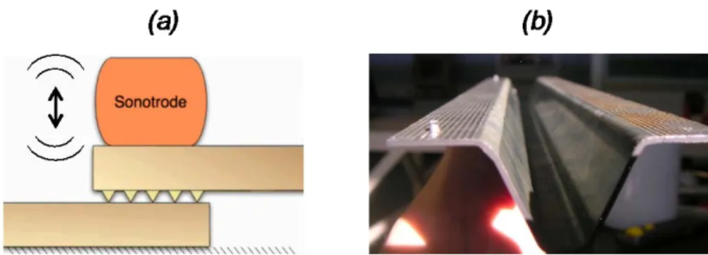
Among the different available welding techniques, ultrasonic welding is of particular interest because of its energy efficiency and rapidity. Furthermore, it does not require the presence of a foreign metallic grid like in resistance or electrofusion welding for example. In this process, in order to achieve the local heating, triangular bulges, called energy directors, are molded on one of the plate to be welded (Figure 13). The assembly is then placed under a tool called sonotrode, which applies simultaneously a constant load and a harmonic ultrasonic compression. The triangular shape is obviously the weakest part of the structure and is thus designed to concentrate the deformation. This localized strain combined with the high loading frequency induces heating because of viscous dissipation [10, 64, 65]. The director then melts and flows at the interface to allow welding, through the formerly described physical mechanisms of intimate contact and macromolecular diffusion.

Figure 13 –Principle of the ultrasonic welding process with molded “energy directors” (a) and picture of a stiffener for aeronautic applications (b).

First results reveal a good mechanical quality of the welding [66]. In particular the advance of the sonotrode enables air removal along the director and avoids the trapping of bubbles. Moreover, it would allow one to assemble large parts using continuous weld lines, where the “static” process (without sonotrode motion) limits the welding area to the size of the

sonotrode. This opens possibilities for this process to be used at an industrial level to assemble large parts keeping an excellent weld quality.

Nevertheless, this technique based on energy directors was not so successful due to the costs of machining and additional surface molding. More recently, an energy director free solution, combining dry friction and viscoelastic heating, was proposed by Villegas [63] and modeled by Levy [62]. It was proved to be efficient and should be also extendable to continuous welding.

5.2 Process modeling: necessity of a time homogenization framework

The main phenomena occurring in this process, initially outlined by Benatar and Gutowski [4] can be summarized as:

(i) mechanics and vibration of the parts, (ii) viscoelastic heating,

(iii) heat transfer, (iv) flow and wetting,

(v) intermolecular diffusion.

Like in every welding process, the modeling of the ultrasonic technique is a complex multi-physical problem implying heat transfer, phase change, thermo-multi-physical evolutions, adhesion, fluid flow, … However, a unique feature of this process is that high frequency of the loading (about 20kHz) that makes any direct calculation unaffordable, especially in regards of the non-linear nature of the multi-physical problem.

To circumvent this problem, a time-homogenization technique was proposed by Levy et al. [59] that provide a mathematically sound basis for such type of problem, to the contrary of more empirical “cycle jump” methods. It takes advantage of the good time scales separation between the welding characteristic time tm ~ 1s and the period of the ultrasonic vibration tµ=50µs, and first introduces the scale separation factor

𝜉 = 𝑡𝜇

𝑡𝑚= 10

−5 _{. Eq. (26)}

Such a good separation is rarely encountered in similar spatial homogenization techniques [67-69] and simply means that problems at short times can probably be well uncoupled from long time ones. All the fields 𝜑 (temperature, displacement, velocity) are then rewritten as double-scale asymptotic expansions in powers of 𝜉:

𝜑(𝒙, 𝑡) = 𝜑0(𝒙, 𝑡, 𝜏) + 𝜉𝜑1(𝒙, 𝑡, 𝜏) + 𝜉2𝜑2(𝒙, 𝑡, 𝜏) + ⋯ , Eq. (27)

where 𝜏 = 𝑡/𝜉 denotes the “fast” time scale. Those expansions are then introduced in the energy and momentum balances and the equations at the different orders of 𝜉 can be identified.

On the basis a simple Maxwell fluid rheological model for the energy directors, Levy et al. [59] showed that the thermo-mechanical problem with a vibrating imposed load can be separated into 3 coupled problems: (i) a thermal problem at long time scale, (ii) a mechanical problem at long time scales that describes the squeezing of the energy directors and (iii) a mechanical problem at short time scales. The latter happens to be an elastic problem; it

results from the very fast loading of the polymer at high frequency, which in that case behaves like a solid. The two first problems are rather classical, except that the heat source of the thermal problem is directly induced by the viscoelastic dissipation resulting from problem (iii). The interest of this approach is that the short times can be solved separately, thus saving a huge amount of time. For example, in the case of a large strain time-dependent problem, the elastic problem for the self-heating can be solved once only every “macro-temporal” time step. It varies only due to the shape change of the domain. The partition into three problems can furthermore be shown to be valid over a wide range of temperature.

5.3 Numerical multi-physical model

Retaining the principle of the theoretical analysis provided by the time homogenization framework, Levy et al. [60] proposed the following set of balance and constitutive equations, dedicated to the simulation of self-heating and squeezing of energy directors made of PEEK:

- Long times mechanical problem: Stokes problem with a power-law fluid, solved in terms of the velocity v ; determination of the shape evolution of the energy director.

𝛁 ∙ 𝛔𝑣_{− 𝛁p = 0 with 𝛁 ∙ 𝐯 = 0 and 𝛔}𝑣 _{= 2𝜂(𝛾̇)}𝑛−1_{𝑫, Eq. (28)}

where 𝛔𝑣 denotes the viscous stress tensor, 𝑫 the strain rate tensor, p the hydrostatic pressure, 𝛾̇ the equivalent shear rate, 𝜂 the consistency and n the power law index. - Short times mechanical problem: elastostatics; determination of vibrations amplitude.

𝛁 ∙ 𝛔𝑒 _{= 0, with 𝛔}𝑒 _{= 𝜆trace(𝝐}𝑒_{) + 2𝜇𝝐}𝑒_{, Eq. (29)}

where 𝛔𝑒 denotes the elastic stress tensor, 𝛜𝑒 the strain tensor, and (𝜆, 𝜇) the Lamé elasticity coefficients.

- Long times thermal problem: heat transfer problem with a source term 𝑄 accounting for the heat produced by self-heating.

𝜌𝜌 �𝜕𝑇_𝜕𝑡+ 𝐯 ⋅ 𝜵𝑇� = 𝛻 ⋅ (𝑘𝜵𝑇) + 𝑄 , with 𝑄 =1₂𝐸′′𝜔𝝐𝑒_{: 𝝐}𝑒_{, Eq. (30)}

where 𝜌 denotes the density, 𝜌 the heat capacity, 𝑘 the conductivity, 𝑇 the temperature field, 𝐸′′, the loss modulus, and 𝜔 = 2𝜋𝑓_{𝑠𝑠𝑛𝑠} the sonotrode pulsation.

Like in most welding processes, obtaining the material data of such multi-physical models is a key problem in order to achieve a realistic simulation tool. As the temperature ranges from room temperature to melting temperature, the thermo-dependence of all parameters have to be thoroughly determined experimentally. Particularly difficult is the determination of the loss modulus 𝐸′′ at 20kHz which is the usual ultrasonic frequency. No conventional apparatus is able to perform such viscoelastic characterization but a time-temperature equivalence is possible, in order to extrapolate results from a classical test at 100Hz [62].

The above-described coupled problem implies an original coupled numerical problem. As explained in [60], the first issue is to handle the large strain of the energy directors. This can be done efficiently by the choice of a Eulerian description (fluid type approach), coupled to a level-set method to describe the evolution of the interface of the flowing energy director. Unlike the two mechanical problems, the thermal problem includes a transient term and an advection term. To simplify the resolution, Levy et al. [60, 61] adopted an operator splitting technique, which provides an efficient way to solve separately the convective part. Following

such an approach, the multi-physical problem formed by equations (28) to (30) can be solved on the domain at time t, either with an iterative or a monolithic approach.

As illustrated in Figure 14, the simulation code developed by Levy et al. [60] is able to produce acceptable physical results compared to experimental observations.

Figure 14: Comparison between a stopped experiment and the reference simulation - temperature field after 0.12 s [60]

5.4 Ultrasonic welding with energy directors: process analysis and optimization

Once the numerical tool is validated, it is possible to use it to better understand the effects of the numerous process and physical parameters: vibration frequency, holding force, welding duration, geometry of the directors.

Figure 15: process analysis and optimization – (a) effect of the holding force on the maximum temperature, (b) effect of the energy director’s tip radius [61].

Figure 15 first focus on the maximum temperature reached in the initial heating stage. Before the glass transition temperature Tg, the value of the holding force has almost no effect because the shape remains the initial one. After Tg, a high holding force is observed to lower the maximum temperature. In fact, it promotes a fast squeezing, but subsequently also rapidly reduces the strain concentration effect. In order to reach the melting temperature as fast as possible, a rather low holding force would be required, contrary to the first intuition. Figure 15(b) illustrates the high importance of the “tip effect”. The strain concentration and subsequent self-heating are directly linked to the sharpness of the energy director. In the limit of what machining would allow, a very tip radius is required.

The effects of triangular directors sharpness is illustrated in Figure 16. In the heating stage (Fig. 16(a)), it is shown that a sharper director promotes a more localized heat generation and

temperature distribution. The consequence on the flow stage is then shown in Figure 16(b). Comparing the flow fronts at t=0.21s, one can check that the sharp director induces a faster flow, and therefore a shorter welding time. Nevertheless, the analysis of flow fronts during squeezing also suggests a higher risk of porosity entrapment. Optimal shapes of those energy directors should therefore combine the antagonist features observed with triangular shapes. They should have a more complex cross section, made of a sharp part, close to the tip, progressively moving into a larger part near the basis.

Figure 16: effect of the geometry of energy directors: (a) temperature distribution and (b) flow front at different instants [61].

Lastly, the classical healing models can also be introduced in such complex simulation tools and provide information about the expectable quality of adhesion. Equation like Eq. (19) is an ODE that can be easily solved on the flow front of the energy director, as soon as it comes in contact with the lower substrate. Provided a representative law for the characteristic time 𝜆(𝑇) and a good calculation of the temperature field, a diffusion criterion or a healing degree can be estimated, as shown in Figure (17).

Figure 16: predicted healing degree for the US welding of PEEK triangular energy directors [61].

6. Conclusion

Optimizing healing of welded thermoplastic material or matrix requires the understanding of physical mechanisms involved in welding processes, which are mainly surface rearrangement and surface approach, wetting of surfaces, macromolecular diffusion and even

co-cristallization at interface of semicrystalline polymers. As it is quite difficult to separate wetting phenomenon from surface rearrangement, as it seems that time scale of wetting phenomenon is one order of magnitude less than surface rearrangement, most of researchers have modelled these two stages into one stage to obtain an the intimate contact, which is necessary to allow macromolecular diffusion. For not fully welded semicrystalline polymers, co-crystallization at interface surely increases the strength of weld lines, but in the state of current scientific knowledge, it is not possible to quantify the role of partial diffusion and co-crystallization in the strength of weld lines. Therefore, it is reasonable for safety reasons of an industrial process to consider that diffusion should be complete before crystallization.

In the last decade, the growing use of thermoplastic matrices inside composite materials has reinforced the interest of the community for the understanding and modeling of the two essential physical phenomena: intimate contact and macromolecular diffusion. As these two physical phenomena are very temperature dependent, precise local temperature measurements or a thermal modelling of processes are necessary to record the thermal history at interfaces in order to quantify these two physical phenomena. As it was shown in this chapter through successful technological applications, those concepts can now be integrated in the modeling of welding processes in order to predict the quality of adhesion in in rather realistic situations. It is rather clear that the theory for describing the healing in that way is becoming rather mature. As thermoplastics may degrade quite quickly in the melted state at high temperature, ie have molecular masses, which vary either by polymer chain cut or crosslinking, molecular mobility is widely modified, therefore intimate contact and diffusion may be affected. Thus, it is important to take into account this possible degradation and to model it to refine processing windows.

Regarding the intimate contact, no model takes into account neither the possible non-Newtonian rheology of the polymer nor the tri-dimensional nature of the surfaces roughness. Though some of them try to account more precisely for the statistical distribution of roughness, the squeezing mechanics remains based on a lubrication assumption, which is questionable. Another critical issue, which was not discussed in this chapter, is the experimental validation of those physical models knowing that the only way to estimate the bonding degree is mechanical testing, often through single lap shear tests or crack opening tests. No in-line measurement of 𝐷_𝑖𝑖, 𝐷_ℎ or diffusion criterion 𝐷 is available, especially at short times. This is the reason why the control of the duration of application of welding pressure and heating should be very precise, which represents an important challenge.

Acknowledgments

The authors acknowledge DGA and EADS for their financial support. We wish to thank Célia Nicodeau, Arthur Levy, Jacques Verdu, Jacques Cinquin and Francisco Chinesta for their contribution to the presented works.

References

[1] R.A. Grimm. Fusion welding techniques for plastics. Welding Journal, 69:23-28, 1990.

[2] C. Ageorges, L. Ye, M. Hou. Advances in fusion bonding techniques for joining thermoplastic matrix composites: A review. Composites Part A: Applied Science and Manufacturing, 32:839-857, 2001

[3] W.I. Lee, G.S. Springer. Interaction of electromagnetic radiation with organic matrix composites.

Journal of Composite Materials, 18:357-386, 1984.

[4] P.K. Yarlagadda, T.C. Chai, An investigation into welding of engineering thermoplastics using focused microwave energy. Journal of Materials Processing Technolology, 74:199-212, 1998. [5] G. Williams, S. Green, J. McAfee, C.M. Heward. Induction welding of thermoplastic composites.

IMechE, C400/034:133-136, 1990.

[6] J.R. Vinson. Adhesive bonding of polymer composites. Polymer Engineering and Science, 29:1325-1331, 1989.

[7] F.N. Cogswell, P.J. Meakin, A.J. Smiley, M.T. Harvey, C. Brooth. Thermoplastic interlayer bonding for aromatic polymer composites. 34th International SAMPE Symposium, 2315-2325,

1989.

[8] Atkison JR, Ward IM. The joining of biaxially oriented polyethylene pipes. Polym Engng Sci 1989;29:1638±41.

[9] N.S. Taylor, M.N Watson. Welding techniques for plastics and composites. Joining & Materials, 1:70-73, 1988.

[10] A. Benatar, T.G. Gutowski. Methods for fusion bonding thermoplastic composites. SAMPE Q:35-42, 1986

[11] R.A. Grimm. Welding processes for plastics. Advanced Material Processes, 147:27-30, 1995. [12] D.M. Maguire. Joining thermoplastic composites. SAMPE J, 25:11-14, 1989.

[13] E. Kenney. Designing plastic parts for ultrasonic assembly. Machine Design, 21:65-68, 1992. [14] R.P. Wool RP, K.M. O'Connor KM. A theory of crack healing in polymers. Journal of Applied

Physics, 52:5953-5963, 1981

[15] C.A. Butler, R.L. Mccullough, R. Pitchumani, J.W. Gillespie. An analysis of mechanisms governing fusion bonding of thermoplastic composites. Journal of Thermoplastic Composite

Materials, 11: 338-363,1998.

[16] J.S.U Schell, J. Guilleminot, C. Binetruy, P. Krawczak, Computational and experimental analysis of fusion bonding in thermoplastic composites: Influence of process parameters.

Journal of Materials Processing Technology, 209: 5211-5219, 2009.

[17] C.-W Tsao, D. DeVoe, Bonding of thermoplastic polymer microfluidics. Microfluidics 
and Nanofluidics, 6:1-16, 2009.

[18] A. Levy, D. Heider, J. Tierney, J.W. Gillespie. Inter-layer thermal contact resistance evolution with the degree of intimate contact in the processing of thermoplastic composite laminates.

Journal of Composite Materials, 48:491-503, 2014.

[19] W.L. Lee, G.S. Springer. A model of the manufacturing process of thermoplastic matrix composites. Journal of composite materials, 21:1017-1055, 1987.

[20] M.B. Gruber, I.Z. Lockwood, T. L. Dolan, S. B. Funck, J. Tierney, P. Simacek, J.W Gillespie, S. Advani, B.J. Jensen, R. J. Cano. Thermoplastic in situ placement requires better impregnated tapes and tows. Proceedings of the 2012 SAMPE Conference. Baltimore, USA, 2012.

[21] P.H. Dara, A.C. Loos. Thermoplastic matrix composite processing model. Virginia Polytechnic

Institute Report, CCMS-85-10: Hampton, VA, 1985.

[22] S.C. Mantell, G.S. Springer. Manufacturing process models for thermoplastic composites.

[23] F. Yang, R. Pitchumani. A fractal Cantor set based description of interlaminar contact evolution during thermoplastic composites processing. Journal of materials science, 36:4661-4671, 2001. [24] F. Yang, R. Pitchumani. Nonisothermal healing and interlaminar bond strength evolution during

thermoplastic matrix composites processing. Polymer Composites, 24:263-278, 2003.

[25] F. Yang, R. Pitchumani. Fractal description of interlaminar contact development during thermoplastic composites processing. Journal of reinforced plastics and composites, 20:536-546, 2001.

[26] T.L. Warren, A. Majumdar, D. Krajcinovic. A fractal model for the rigid-perfectly plastic contact of rough surfaces. Journal of Applied Mechanics, 63:47-54, 1996.

[27] F. Yang, R. Pitchumani. Interlaminar contact development during thermoplastic fusion 
bonding.

Polymer Engineering and Science, 42:424-438, 2002.

[28] Y. Chen, P. Fu, C. Zhang, M. Shi. Numerical simulation of laminar heat transfer in microchannels with rough surfaces characterized by fractal Cantor structures. International Journal of Heat and

Fluid Flow, 31:622-629, 2010.

[29] F. Sonmez, H. Hahn. Analysis of the on-line consolidation process in thermoplastic composite tape placement. Journal of Thermoplastic Composite Materials, 10:543, 1997.

[30] C. Nicodeau. Modélisation du soudage en continu des composites à matrice thermoplastique. PhD thesis, Ecole Nationale Supérieure d’Arts et Métiers de Paris, http://tel.archives-ouvertes.fr/ pastel-00001506, 2005.

[31] J.-F. Lamethe, P. Beauchene, L. Leger. Polymer dynamics applied to PEEK matrix composite welding. Aerospace Science and Technology, 9(3):233–240, 2005.

[32] J. Tierney, J. W. Gillespie. Modeling of in situ strength development for the thermoplastic composite tow placement process. Journal of Composite Materials, 40:1487–1506, 2006.

[33] P.J. Flory. X. The Configuration of Real Polymer Chains. Journal of Chemical Physics, 17:303-310, 1949.

[34] M. Rubinstein, R.H. Colby, Polymer physics. Oxford University Press, Oxford, 2003. [35] L. J. Fetters, D. J. Lohse, R. H. Colby. Chapter 25: Chain Dimensions and Entanglement

Spacings. In J.E. Mark, editor, Physical Properties of Polymers Handbook –Second Edition, 445-452. Springer, New York, 2007.

[36] P.E. Rouse. A theory of the linear viscoelastic properties of dilute solutions of coiling polymers.

Journal of chemical physics, 55:572-579, 1971.

[37] L.J. Fetters; D.J. Lohse, S.T. Milner, W.W. Graessley. Packing length influence in linear polymer melts on the entanglement, critical, and reptation molecular weights. Macromolecules, 32:6847-6851, 1999.

[38] P.G. de Gennes. Reptation of o polymer chain in the presence of fixed obstacles. Journal of chemical physics. 55 :572-579, 1971.

[39] P.G. de Gennes. Scaling Concepts in Polymer Physics. Cornell University Press, New-York, 1979.

[40] H.H. Kausch, M. Tirrell. Polymer interdiffusion. Annual Review of Materials Science, 19: 341-377, 1989.

[41] R.P. Wool, K.M. O’Connor. A theory of healing at a polymer interface. Macromolecules, 16:1115-1120, 1983.

[42] R.P. Wool, B.L. Yuan, O.J. McGarel, Welding of polymer interfaces. Polymer Engineering and

Science, 29:1340-1367, 1989.

[43] F. Yang, R. Pitchumani. Healing of thermoplastic polymers at an interface under nonisothermal conditions. Macromolecules, 35: 3213-3224, 2002.

[44] Y.-Q Xue, T.A. Tervoort, S. Rastogi, P.J. Lemstra. Welding behavior of semicrystalline polymers. 2. Effect of cocrystallization on autohesion. Macromolecules, 33:7084-7087, 2000. [45] B.L. Yuan, R.P. Wool. Strength development at incompatible semicrystalline polymer interfaces.

[46] A. Gent, E.G. Kim, P. Ye. Autohesion of crosslinked polyethylene. Journal of Polymer Science

Part B: Polymer Physics, 35:615-622, 1997

[47] B. Fayolle, L. Audouin, J. Verdu. Radiation induced embrittlement of PTFE. Polymer, 44:2773-2780, 2003.

[48] W.W. Graessley. The entanglement concept in polymer melt rheology. Advances in Polymer

Science, 16:1–179, 1974

[49] J.D. Ferry, Viscoelastic properties of polymers- 3rd ed. Wiley, New York, 1980.

[50] E. van Ruymbeke, C.-Y. Liu, C Bailly. Quantitative tube model predictions for the linear viscoelasticity of linear. Rheology Reviews, 53 – 134, 2007.

[51] W.W. Graessley. Some phenomenological consequences of the Doi–Edwards theory of viscoelasticity, Journal of Polymer Science. Phys. Ed., 18:27–34, 1980.

[52] J.E Zanetto, C.J.G Plummer, J.A. Manson. Fusion bonding of polyamide 12, Polymer

Engineering and Science, 41:890-897, 2001

[53] G. Régnier, C. Nicodeau, J. Verdu, J. Cinquin, F. Chinesta. A multi-physic and multi-scale approach to model the continuous welding of thermoplastic matrix composites, Proceedings of ICCM16, Kyoto, Japan, 2007.

[54] C. Coiffier-Colas, H. Sibois, P. Lefebure. Future for high performance thermoplastic composites and aircraft helicopters, Proceedings of JEC Composites, Paris, 14-19, 2005.

[55] C. Nicodeau, G. Régnier, J. Verdu, F. Chinesta, V. Triquenaux, J. Cinquin. Welding of thermoplastic matrix composites: prediction of macromolecules diffusion at the interface.

Proceedings of the 8th ESAFORM conference, Cluj Napoca, Roumania, 897-900, 2005.

[56] D. Saint-Royre, D. Gueugnaut, D. Reveret. Test methodology for the determination of optimum fusion welding conditions of polyethylene. Journal of Applied Polymer Science, 38:147–162, 1989.

[57] M. Day, J.D. Cooney, D.M. Wiles. Kinetic study of the thermal decomposition of poly(aryl-ether-ether-ketone) (PEEK) in nitrogen. Polymer Engineering and Science, 29:19-22, 1989.

[58] K.G. Cole, I.G. Casella. Fourier transform infra-red spectroscopic study of thermal degradation in poly(ether ether ketone)-carbon composites. Polymer, 34:740-745, 1993.

[59] A. Levy, S. Le Corre, A. Poitou, E. Soccard. Ultrasonic welding of thermoplastic composites, modeling of the process using time homogenization, Int J. Multiscale Comput. Engrg, 9:53-72, 2011.

[60] A. Levy, S. Le Corre, N. Chevaugeon, A. Poitou. A level set based approach for the finite element simulation of a forming process involving multiphysics coupling: ultrasonic welding of thermoplastic composites. European Journal of Mechanics, 9:501-509, 2011.

[61] A. Levy, S. Le Corre, A. Poitou, Ultrasonic welding of thermoplastic composites: a numerical analysis at the mesoscopic scale relating processing parameters, flow of polymer and quality of adhesion, Int. J. Material Forming, 7:39-51, 2014.

[62] A. Levy, S. Le Corre, I. Fernandez-Villegas, Modelling of the heating phenomena in ultrasonic welding of thermoplastic composites with flat energy directors, J. Materials Processing

Technology, 214:1361-1371, 2014.

[63] I.F. Villegas. In situ monitoring of ultrasonic welding of thermoplastic composites through power and displacement data. Journal of Thermoplastic Composite Materials, 24:1007-1024 (2013). [64] C. Nonhof, G. Luiten. Estimates for process conditions during the ultrasonic welding of

thermoplastics. Polym Eng Sci, 36:1177-1183, 1996.

[65] M.N. Tolunay, P.R. Dawson,, K.K Wang. Heating and bonding mechanisms in ultrasonic welding of thermoplastics. Polym Eng Sci, 23:726–733, 1983.

[66] E. Soccard. Ultrasonic assembly method. Patent number: WO 2007/003626 A1 WO 2007/003626 A1, EADS CCR, 2007.

[67] A. Bensoussan, J.-L. Lions, G. Papanicolaou. Asymptotic Analysis for Periodic Structures. North-Holland, Amsterdam, 1978.

[68] N.S. Bakhvalov, B. Panasenko. Homogenisation: averaging processes in periodic media— mathematical problems in the mechanics of composite materials. In Mathematics and its

Applications Soviet Series, 36. Kluwer Ac. Publishers, Dordrecht–Boston–London, 1989.

[69] G. Moreau, D. Caillerie. Continuum modeling of lattice structures in large displacement framework. Dev. Comput. Tech. Struct. Eng, 20;53–70, 1995.