Plant Monitoring and Fault Detection
Synergy between Data Reconciliation and Principal Component Analysis.
Th. Amand a, G. Heyen a, B. Kalitventzeff b[email protected], [email protected], [email protected]
a L.A.S.S.C., Université de Liège, Sart-Tilman Bâtiment B6a, B-4000 Liège (Belgium) b Belsim s.a., 1 Allée des Noisetiers, B-4031 Angleur - Liège (Belgium)
Abstract : Data reconciliation and principal component analysis are two recognised statistical methods used for plant monitoring and fault detection. We propose to combine them for increased efficiency. Data reconciliation is used in the first step of the determination of the projection matrix for principal component analysis (eigenvectors). Principal component analysis can then be applied to raw process data for monitoring purpose. The combined use of these techniques aims at a better efficiency in fault detection. It relies mainly in a lower number of components to monitor. The method is applied to a modelled ammonia synthesis loop.
1. INTRODUCTION
Measurements are needed to monitor process efficiency and equipment condition, but also to take care that process parameters remain within acceptable range to ensure good product quality, avoid equipment failure and any hazardous operation.
Model based statistical methods, such as data reconciliation, are provided to analyse and validate plant measurements. The objective of these algorithms is to remove any error from available measurements, and to yield complete estimates of all the process state variables as well as of unmeasured process parameters. Besides that, algorithms are needed to detect faults, i.e. any unwanted, and possibly unexpected, mode of behaviour of a process component (Cameron 1999). In practice, the following faults need to be detected and diagnosed in the process industries:
• Equipment failures and degradations. • Product quality problems.
• Internal deviations from safe or desired operation (hot spots, pressure rises).
Fault detection and diagnosis is generally accepted to occur in three stages: 1. Detection - has a fault occurred?
2. Identification - where is the fault? 3. Diagnosis - why has the fault occurred?
The goal of our study is to examine how two well accepted techniques, data reconciliation (DR) and principal component analysis (PCA), can work in conjunction to enhance process monitoring.
2. PRINCIPAL COMPONENT ANALYSIS
Any process is affected by variability, but process variables do not fluctuate in a completely random way. These are linked by a set of constraints (mass and energy balances, operating policies) that can be captured in a process model. Even if a rigorous mathematical model is not available, statistical analysis of the process measurements time series can reveal underlying correlation between the measured variables (Kresta et al, 1991).
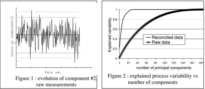
If measurements related to abnormal conditions are removed from the analysed set, the principal components of the covariance matrix (i.e. the eigenvectors associated with the largest eigenvalues) correspond to the major trends of normal and accepted variations. Most of the variability in the process variables can usually be represented by the first few principal components, which span a subspace of lower dimension corresponding to the normal process states (Snedecor G., 1956). Projection of new measurements point in this subspace is expected to follow a Gaussian distribution, and can be checked for deviations from their mean values using the usual statistical tests (example in figure 1).
With this approach, one can verify whether a new measurement belongs to the same distribution as the previous sets that were recognised as normal. If not, a fault is likely to be
-25 Data set S c o r e o n c o m p o n e n t : 2
Figure 1 : evolution of component #2, raw measurements 0 0.2 0.4 0.6 0.8 1 1 21 41 61 81 101 121 141 161 181
number of principal components
E xp la in ed v ar ia bi lit y Reconciled data Raw data
Figure 2 : explained process variability vs number of components
the cause; it can result from an excursion out of the normal range of operation, or from an equipment failure breaking the normal correlation between the process variables. It can also result from normal operation in conditions that were not covered in the original set used to determine the principal component basis.
3. DATA RECONCILIATION
The underlying idea in DR is to formulate the process model as a set of constraints (mass and energy balance, some constitutive equations). All measurements are corrected in such a way that reconciled values do not violate the constraints. Corrections are minimised in the least square sense, and the measurement accuracy is taken into account by using the measurement covariance matrix as a weight for the measurement corrections.
Sensitivity analysis can be performed and is the basis for the analysis of error propagation in the measurement system (Heyen et al, 1996). With this technique, variations of some state variables can be linked to deviations in any measurement.
A drawback of DR is the presence of a gross process fault (e.g. a leak): since the basic assumption of data reconciliation is the correctness of the model, it is efficient to detect and correct failing sensors, but it may be less adequate to detect process faults. In this case, the
DR procedure will tend to modify correct measurements while in fact there is a mismatch between the model and the actual process.
4. PRESENTATION OF A COMBINED DETECTION METHOD 4.1. Projection Matrix
The PCA orthogonal projection matrix is the key point of the fault detection method. In order to determine it, one might use either a raw data set, or reconciled values. The number of significant principal components (PC) obtained by way of the projection matrix determined
with both data sets is very different. Taking into account more components allows explaining a higher fraction of the total process variability, as shown in figure 2 for an example with 186 variables. When using raw measurements to determine the projection matrix, a large number of components is needed to explain most of the process variability (upper limit is the number of original variables).
When using the reconciled data sets, the number of significant PC remains much smaller than the number of state variables (the upper limit is the number of degrees of freedom of the data reconciliation model). This reduction in the problem size allows the system monitoring with only a few PC. The DR technique applied to the raw data sets has somewhat filtered them and reduced the noise.
Furthermore, since data reconciliation enforces the strict verification of all mass and energy balance constraints, the linear combinations captured in the projection matrix are truly representative of realistic models. For example, the mass balance of a simple mixer is represented by the equation:
F1+F2=F3
with F1 and F2 as the inlet and F3 as the outlet flowrates, while statistical analysis of noisy measurements would lead to a correlation such as:
a . F1 + b . F2 = F3
where coefficients a and b would probably differ from 1. Using DR as a preprocessor will ensure that the PC represent the proper process behaviour. For later analysis, we will thus use the projection matrix obtained from the reconciled values.
4.2. Confidence limits
The number of measurement sets corresponding to normal conditions has to be large enough in order to span all causes of process variability and to avoid spurious fault detection
(i.e. in case of conditions that are acceptable, but were not available in the training set). A confidence limit has to be chosen to determine the number of PC to be used : choosing a 100% confidence level would be equivalent to use all the PC. This would be the same as monitoring as many variables as the number of primary variables. The choice of the number of PC is a compromise between security and simplicity : a lower number of PC is easier to watch. Nevertheless, a small number of PC will decrease the sensitivity of the method.
Confidence limits are calculated on the base of a normal distribution for each of the PC. This limit will be used for fault detection purpose. A lower confidence limit on a component increases the sensitivity: potential faults are detected earlier, but erroneous detection is more frequent. The measurement precision must also be taken into account for the determination of these limits. When measurements are affected by large random errors, a fault can be detected even when there is no actual problem on the process.On the other side, a too large confidence limit will delay or even inhibit fault detection. Thus repeated excursions of the component beyond the fixed limits will be needed to flag a fault.
5. CASE STUDY : AMMONIA SYNTHESIS LOOP 5.1. Primary model and reference data sets
A simulation model of an ammonia synthesis loop has been used to generate pseudo measurements. The model involves 186 state variables.
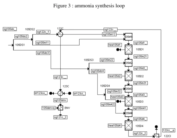
Only the inner part of the synthesis loop (figure 3) and the reactor (figure 4) models are taken into account.
Figure 3 : ammonia synthesis loop
A set of 210 reference operating conditions has been obtained by solving the simulation model repeatedly with varying specifications. The specifications were generated randomly from a Gaussian distribution. Variables assumed to be measured were then corrupted with a random noise of known distribution. Each raw data set generated in this way was also processed using VALI III data reconciliation package (Belsim 1999). In the present case study, we selected a number of PC allowing to represent 95 or 99% of the process variability. This corresponds to the first 20 and 27 PC (figure 2). Figure 1 shows an example of 90% and 95% confidence limits for the second principal component obtained from the raw reference data set, compared to its contribution in each of the 210 test cases. The null mean value of the component is also represented. A similar graph can be obtained from reconciled data.
5.2. Simulation of a fault in process operation
Data sets corresponding to process faults of variable severity have also been generated with a model modified to represent an equipment fault. The altered model is first set with specifications leading to no fault at all. A data set is generated by solving the simulation model with random variations of the specifications, but with the fault effect becoming progressively larger. The measured variables are corrupted with normally distributed noise. A data reconciliation procedure, based on the primary, fault free model, is also applied to the data.
A faulty data set is composed of time series of measurements of all the state variables. In the case of a leak, the leak flow is initially set to zero for the first element of the series, and its value is gradually increased with time. In this way, it is possible to evaluate the PCA fault detection method by analysing how quickly and how trustfully it responds to a problem arising in the ammonia loop.
As a single excursion of a component out of its limits is not enough to detect safely the presence of a fault in the process. An error is only flagged when a component remains out of bounds during several consecutive steps.
In this study, we identified the time at which a fault had been detected as the time a PC left its confidence limits to remain permanently out of bounds. The confidence limit for each component has been set to 99%, because the 95% value proved to be too sensitive and lead to spurious fault detection.
Different fault types were generated for this study : internal leak in a proces-to-process heat exchanger, leak between process gas and utility, leak to the ambient, catalyst deactivation in the reactor.
5.3. Internal leak in a heat exchanger
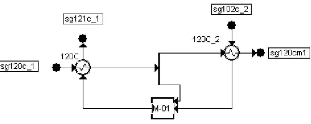
In order to simulate the appearance of a leak in a heat exchanger, we modified the model according to figure 5. The exchanger is split in two halves, and part of the tube-side stream is split and mixed with the shell-side stream.
Figure 5 : modelling a leak in a heat exchanger
In the case of a leak in the reactor product to feed heat exchanger, analysis of ten different time series gives the results in table 1. Principal component number 4 is the first to drift out of its confidence limits, both when using raw or reconciled values.
Raw Data Mean time 6.8 9.5 11.8 11.9 12 13.8 16.9 17.9 18.1 18.4 Component 4 3 1 5 2 23 24 27 8 25 Reconciled data Mean time 6.6 11.6 15.6 19 19.8 20.7 20.9 20.9 20.9 21 Component 4 1 5 2 3 21 8 11 23 6 Table 1
The analysis of the correlation matrix between the state variables and the principal components allows locating the fault on the process. The fourth component is much correlated to the temperature of one the streams coming out of the exchanger. The NH3 composition of the other stream is also modified. On the five first variables correlated to this component, two more are related to flows connected to the liquid ammonia separator. In the average, the fault has been detected for the seventh data set, and it corresponds to a leak of 6% of the gas flow. 5.4. Exchanger leak between process and utility flows
In this case, the leak is simulated in exchanger cooling the synthesis gas with liquid ammonia. This exchanger has been selected because it operates in parallel with another branch of the main loop. To model the leak, the original exchanger has been split in two smaller units performing the same duty when the leak vanishes. Table 2 shows that 4 principal components drift out of their confidence limits almost immediately. The analysis based on reconciled data flags the error somewhat earlier. The major PC implied are numbered 3, 7, 8 and 4. The large number of PC involved simultaneously in the fault detection makes it difficult to locate precisely the cause of the fault. The detection method has been modified to get more information from the data sets. For each time step t, a composite index It is determined for each measured variable. It is obtained by summing up over a time horizon the score of all principal components drifting out of bounds, weighted by the variable
contribution in the corresponding eigenvector. This index reveals any repeated departure from average for the variables mostly correlated with the drifting components. Applying this test in the previous example indicated that suspect variables were the partial flows of nitrogen and argon in the ammonia produced and the partial flow of hydrogen in the reactor feed and the reactor effluent. Raw data Mean time 2 2 2 2.1 2.2 2.2 2.8 3.4 3.6 3.8 Component 3 7 8 4 2 6 1 23 11 19 Reconciled data Mean time 2 2 2 2 2.1 2.1 2.7 3.1 3.6 3.9 Component 3 4 7 8 2 6 1 23 19 11 Table 2
Monitoring the sign of the measurement deviations is also indicative. In our example, nitrogen and argon flowrates appear to decrease in the separator outlet, while hydrogen is rising in the reactor effluent. The temperature of the recycled flow is decreasing. Overall, the hydrogen partial molar flow is increasing in the reactor as well as the temperature. From all these observations it seems difficult to locate the fault in the process. However, a leak to the ambient can be considered, to explain the decrease of the inert (argon) flow rate in the loop. The mean detection time varies between 3 and 4, which corresponds respectively to leaks of 0.1 and 0.15 % from the synthesis gas flow. A fault is quickly detected but identification of the exact cause is not easy with the available data.
5.5. Direct leak to the ambient
This case is quite similar to the previous one. Both leaks can be assumed to a loss of matter in the loop. The measurements associated with the earliest fault detection are the same as for
the previous case. The partial molar flow rate of ammonia at the outlet of the separator is also increasingly involved with time.
Once more the method is able to detect the occurrence of the fault but the location of its cause is not possible. Early detection is achieved though, already for the 3rd data set, corresponding to a leak of 0.1% of the sg120cs flowrate.
It should be noticed that the data sets were obtained from independent steady state simulations. Thus they do not account for dead times usually observed in actual process operations. In a steady state models, on all the variables are simultaneously affected by any fault. We did not consider here the effect of dead times in fault propagation, nor the influence of measurements frequency.
5.6. Catalyst deactivation
The catalyst deactivation was taken into account by way of the “departure from the equilibrium temperature” approach. In this way, the effect of reaction rate limiting the extent is represented by calculating the equilibrium at a temperature differing from the reactor outlet temperature. The equilibrium departure is positive for exothermic reactions and negative for endothermic reactions in order to avoid the reaction extent to exceed the equilibrium.
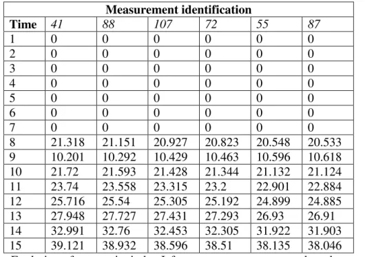
In this case, the raw and reconciled data sets are very different. For the raw data, the PCA detection method indicates that the hydrogen partial molar flow in sg122c, in sg105m41, in sg105d4, in sg105m31, in sg105m21 (i.e. variables 41, 88, 107, 72 and 55) are involved. The partial molar flow in sg105d3 (var. 87) is also suspected during the detection. The detection occurs for measurement set #9, corresponding to a drop from 23.0K to –16.7K of the equilibrium departure ∆T in the second catalyst bed. Table 3 shows the direction of evolution
Measurement identification Time 41 88 107 72 55 87 1 0 0 0 0 0 0 2 0 0 0 0 0 0 3 0 0 0 0 0 0 4 0 0 0 0 0 0 5 0 0 0 0 0 0 6 0 0 0 0 0 0 7 0 0 0 0 0 0 8 21.318 21.151 20.927 20.823 20.548 20.533 9 10.201 10.292 10.429 10.463 10.596 10.618 10 21.72 21.593 21.428 21.344 21.132 21.124 11 23.74 23.558 23.315 23.2 22.901 22.884 12 25.716 25.54 25.305 25.192 24.899 24.885 13 27.948 27.727 27.431 27.293 26.93 26.91 14 32.991 32.76 32.453 32.305 31.922 31.903 15 39.121 38.932 38.596 38.51 38.135 38.046
Table 3 : Evolution of composite index It for suspect measurements, based on raw data There is an overall rise of the partial molar flow of hydrogen. The order of detection starts from the outlet of the reactor and goes up the different catalyst beds. One can assess a conversion loss in the reactor. More, as the temperature does not seem to be involved, a catalyst deactivation is expected. However, the precise location of the problem within the reactor is not possible.
A similar treatment has been carried out based on reconciled measurements. Results are shown in table 4. The detection occurs later, and is only confirmed for the 14th data set (∆T
65K). More measurements are reported as suspect. It is impossible to determine in this case which measurements are involved in the fault. Variables 146, 168, 166, 49, 102 and 68 all show a temperature increase in the loop, and variables 119 and 52 seem to indicate an ammonia flowrate larger than usual, which is the opposite phenomenon to the one simulated. DR is not effective in this case.
Measurement identification Time 146 168 166 164 119 52 49 102 68 1 0 0 0 0 0 0 0 0 0 2 0 0 0 0 0 0 0 0 0 3 0 0 0 0 0 0 0 0 0 4 0 0 0 0 0 0 0 0 0 5 0 0 0 0 0 0 0 0 0 6 0 0 0 0 0 0 0 0 0 7 0 0 0 0 0 0 0 0 0 8 0 0 0 0 0 0 0 0 0 9 0 0 0 0 0 0 0 0 0 10 9.883 9.731 9.731 9.731 8.767 8.766 7.051 7.051 7.051 11 -0.265 0.519 0.519 0.517 1.492 1.492 1.369 1.369 1.369 12 0 0 0 0 0 0 0 0 0 13 10.082 9.927 9.927 9.927 8.943 8.943 7.193 7.193 7.193 14 12.601 12.407 12.407 12.408 11.178 11.178 8.990 8.990 8.990 15 13.597 13.426 13.426 13.424 11.654 11.654 1.798 1.798 1.798 16 11.107 10.937 10.937 10.937 9.851 9.852 7.924 7.924 7.924 Table 4 : Evolution of composite index It for suspect measurements, based on reconciled data The cause of this counter-intuitive behaviour can be traced in the way the reactor was modelled. Since the catalyst efficiency in each bed of the reactor is represented by the departure from equilibrium temperature concept, the lower production in the faulty second bed is partially compensated in the following beds. A more realistic simulation of the effect of kinetics is needed to evaluate the performance of the detection method in this case.
6. CONCLUSION
The fault detection method exposed here, by combining data reconciliation with PCA, is promising. The first benefit is to reduce the number of variables needed to monitor the process. The monitoring of the process is made easier and the computing demand is decreased. The PCA method does not require any type of distribution of the original variables.
However, the detection method is based on confidence regions estimated from a normal distribution.
The proposed method of fault identification is a two step procedure. First a fault is detected when the score of a new measurement set results in some components lying out of their confidence region. In a next step, the effect of the latter components on the original variables is calculated. This allows sorting out the more altered variables, which are likely to be linked to the primary cause of the fault.
Data reconciliation is recommended as a preliminary filtering step before the determination of the PCA projection matrix and the PCA correlation matrix between the PC and the original variables. These matrices are determined only once on the basis of the reference data set. If the raw data were to be used for the determination of these matrices, a larger number of components would be needed to represent the data variability at the same confidence level, but the least significant components would be much affected by noise.
However raw data should be used when using the method to detect faults. DR allows filtering of some data such as faults from measuring devices, and is likely to impede detection of a fault by correcting measurements. The quality of the model used is here very important.
Overall, the fault detection method by principal component analysis is effective in all the cases studied here. The sensitivity of the method can be adjusted thanks to the confidence regions for each component. This method is a priori relevant to any kind of process. The precise identification of the fault location is not always possible. But one should remind that this study is only based upon simulated data. Taking into account the process dynamics and dead times in fault propagation might improve the capabilities of the method if measurements are sensitive and fast.
REFERENCES
Cameron D, Fault Detection and Diagnosis, in "Model Based Manufacturing - Consolidated Review of Research and Applications", document available in CAPE.NET web site (http://capenet.chemeng.ucl.ac.uk/ ) (1999)
Heyen G. , Maréchal E. , Kalitventzeff B., Sensitivity calculations and variance analysis in plant measurement reconciliation, Computers and Chemical Engineering, vol. 20S, pp 539-544 (1996).
Kresta J.V., MacGregor J.F, Marlin T.E., "Multivariate statistical Monitoring of Process Performance", The Canadian Journal of Chemical Engineering, 69, 35-47 (1991)
BELSIM, VALI III Users Guide, BELSIM sa, Allée des Noisetiers 1, 4031 Angleur (Belgium) (1999)