Faculty of Applied Sciences
Doctoral Thesis
Power Line Conductors, a
Contribution to the Analysis of
their Dynamic Behaviour
Suzanne Gu´
erard
Supervisor:
Prof. Jean-Louis Lilien
June, 2011
Faculty of Applied Sciences
Doctoral Thesis
Power Line Conductors, a
Contribution to the Analysis of
their Dynamic Behaviour
Suzanne Gu´
erard
Supervisor:
Prof. Jean-Louis Lilien
June, 2011
Copyright c
University of Li`ege
All rights reserved
Abstract
All the chapters of this thesis are linked with the concern of aeolian vibra-tion. At locations where the motion of overhead power line conductors is restrained (e.g. at suspension clamps), the presence of aeolian vibration may result in another phenomenon called “fatigue of overhead conductors”. The latter being responsible for serious damage to overhead power lines. The first part of the document is devoted to a review of the basic concepts of aeolian vibration and fatigue, of the tools available to model, measure or predict vibrational damage, and what are the remedial measures.
In a second part, a series of experimental studies are related:
• A review of the usual fatigue indicators, based on measurements per-formed on a 63.5m laboratory test span (chapter 2). The aim is to better understand how to perform a correct vibration risk analysis, knowing e.g. what to measure and at which locations.
• An evaluation of conductor self-damping properties based on real out-door measurements, using a new type of monitoring device, able to perform continuous measurement on power lines (chapter 3). Unlike laboratory tests, such on-site measurements permit to take into ac-count e.g. the effect of span ends, the spatial and time fluctuations in wind, leading to a more realistic vibration risk assessment.
• A study of the vibratory pattern associated to the failure of a conduc-tor wire1 (chapter 4). If not detected early, the presence of conductor fatigue may eventually lead to the failure of some conductor wires. This chapter investigates the possibility to detect such an event and eventually to use it as a fatigue indicator.
The third part of the thesis gathers modelling studies, starting with a few basic model validations (chapter 5), which permit to understand some interesting phenomena observed experimentally and to highlight the pres-ence of amplitude fluctuations in the computed time response. The latter are believed to be linked to tension fluctuations. The hypothesis is further developed in chapter 6, comparing the results of constant versus variable
1
tension models and discussing the potential impact of tension fluctuations, when the vibrational behaviour of a real line is being extrapolated from tests performed on laboratory test spans. The modelling part ends up with the mining of experimental curves measured at University of Li`ege by A. Go-dinas [28] (chapter7). Once this input has been adequately processed, the followings have been achieved,
• A formula to compute the self damping per unit length within the conductor has been deduced. The predicted self damping values are consistent with those deduced from the literature, using more compli-cated measurement techniques,
• The parameters of an equivalent viscoelastic material have been de-duced. Once implemented within a non-linear beam element, it per-mits to model both the conductor variable bending stiffness and self damping properties,
• A new method is proposed to measure the conductor self damping properties. The required test set-up is the one used by Godinas. The proposed method is much simpler than others already published in the literature in the sense that: the load can be applied quasi-statically, only a limited number of measurements is required, the test set-up is simple, simple to operate, less expensive than others... The perspective shown by this work is the following: knowing the conductor properties and the shape of some moment versus curvature cycles, the proposed formula would permit to estimate the conductor self damping in any kind of aeolian vibration without any dynamic testing.
In the last and fourth part of this chapter, the modelling results have been compared to experimental ones. To be more precise, the compatibility between the conductor variable bending stiffness deduced in chapter 7 and other results either published in the literature or measured by the author is checked in chapter 8. Then, chapter 9 illustrates the difficulties faced to reproduce resonance conditions on an experimental test bench. Some of them could be due to tension fluctuations. Last, in chapter 10, an energy balance is used to figure the order of magnitude of the self-damping due to non linearities.
Abstract
Le point commun qui unit les chapitres de cette th`ese est le souci des vibra-tions ´eoliennes. Aux endroits o`u le mouvement des conducteurs de lignes a´eriennes est entrav´e, la pr´esence de vibrations ´eoliennes peut engendrer un autre ph´enom`ene, appel´e “fatigue des conducteurs”, et pouvant occasionner d’importants d´egˆats.
La premi`ere partie du document est consacr´ee `a une pr´esentation des concepts de base li´es `a la fatigue des conducteurs et aux vibrations ´eoliennes, aux outils permettant de mod´eliser ces ph´enom`enes ou de les quantifier, ainsi qu’aux mesures “curatives”, permettant d’´eviter ce ph´enom`ene ou de limiter son impact.
Dans la seconde partie, une s´erie d’´etudes exp´erimentales sont relat´ees: • Une ´etude comparative des indicateurs usuels de fatigue, bas´ee sur
des mesures effectu´ees sur une port´ee de laboratoire de 63.5m de long (chapitre 2). L’objectif de cette ´etude ´etant de mieux comprendre com-ment r´ealiser une analyse de risque vibratoire correcte, par exemple en sachant `a quelles mesures proc´eder, et `a quels endroits.
• Une ´etude des propri´et´es d’auto-amortissement de conducteurs, bas´ee sur des mesures r´ealis´ees sur de vraies port´ees, en environnement ext´erieur (chapitre 3). Les mesures ont ´et´e r´ecolt´ees `a l’aide d’un nouveau type d’appareil, capable d’effectuer des mesures en continu sur des lignes a´eriennes. Contrairement aux essais r´ealis´es en labo-ratoire, les mesures sur site permettent de prendre en compte entre autres l’effet des extr´emit´es de port´ee sur les vibrations, les fluctua-tions temporelle et spatiale de vent, ce qui conduit `a une estimation plus r´ealiste du risque vibratoire.
• Une ´etude de la signature vibratoire associ´ee `a une rupture de brin2. Si le ph´enom`ene de fatigue n’est pas d´etect´e `a temps, celui-ci peut con-duire `a la rupture de brins et mˆeme du conducteur. Dans le chapitre 4, la possibilit´e d’arriver `a d´etecter les ruptures de brins est ´etudi´ee, avec en point de mire son utilisation comme indicateur de fatigue. 2
La troisi`eme partie du document rassemble diff´erents r´esultats de mod´elisation, qui permettent de comprendre certains ph´enom`enes observ´es exp´erimentalement, et de mettre en ´evidence la pr´esence de fluctuations d’amplitudes dans la r´eponse du conducteur (chapitre 5). Le document prend pour th`ese que ce sont des variations de traction qui g´en`erent ces fluctuations. La th`ese est d´evelopp´ee plus en d´etails dans le chapitre 6, o`u les r´esultats de simulations `
a traction variable et constante sont compar´es. Ce chapitre discute aussi l’impact potentiel des fluctuations de traction, lorsque des r´esultats d’essais r´ealis´es sur de courtes port´ees de laboratoire sont extrapol´es pour pr´edire le comportement de lignes r´eelles. La partie “mod´elisation” s’ach`eve sur l’exploitation de courbes expr´erimentales mesur´ees `a l’ULg par A. Godinas (chapitre 7). Une fois ces donn´ees trait´ees de mani`ere ad´equate, les r´esultats suivants ont ´et´e obtenus:
• Une formule pour calculer la puissance dissip´ee par unit´e de longueur dans les conducteurs a pu ˆetre d´eduite. Les valeurs fournies par la formule sont coh´erentes avec celles d´eduites de la litt´erature, qui se basent sur des techniques de mesure plus complexes.
• Les param`etres d’un mod`ele de mat´eriau visco´elastique ´equivalent au conducteur ont pu ˆetre d´eduits. Une fois ce mat´eriau introduit dans un ´el´ement de poutre non lin´eaire, il devrait permettre de mod´eliser `a la fois l’amortissement et la rigidit´e en flexion variable du conducteur. • Une nouvelle m´ethode est propos´ee pour mesurer les propri´et´es d’auto amortissement des conducteurs, utilisant le dispositif d’essais de Go-dinas. La m´ethode propos´ee est beaucoup plus simple que d’autres, dans le sens o`u les essais peuvent ˆetre r´ealis´es de mani`ere quasi statique (les autres m´ethodes requi`erent des essais dynamiques), le dispositif d’essais est simple, simple `a manipuler, moins cher que d’autres... La perspective offerte par cette nouvelle m´ethode est la suivante: connais-sant les caract´eristiques du conducteur et quelques courbes moment en fonction de la courbure, l’auto amortissement du conducteur soumis `
a n’importe quelle amplitude ou fr´equence de vibration ´eolienne de-vrait pouvoir ˆetre estim´e par la formule sans devoir r´ealiser d’essais dynamiques.
Dans la derni`ere et quatri`eme partie de la th`ese, les r´esultats obtenus par mod´elisation sont compar´es `a d’autres r´esultats exp´erimentaux. De mani`ere plus pr´ecise, la compatibilit´e entre la rigidit´e en flex-ion variable d´eduite au chapitre 8 et d’autres r´esultats publi´es est v´erifi´ee. Dans le chapitre 9, les difficult´es de r´ealiser l’ajustement en-tre fr´equence d’excitation et de r´esonance au laboratoire sont illustr´ees. Certaines de ces difficult´ees pourraient ˆetre attribu´ees aux variations de traction. Pour finir, au chapitre 10, un bilan ´energ´etique est utilis´e
pour estimer l’ordre de grandeur de la puissance dissip´ee par les non-lin´earit´es.
Contents
List of symbols 1
Acknowledgements 3
Introduction 5
I Bibliography 7
1 State of the art 9
1.1 When it all began . . . 9
1.2 Dangerous conditions and aeolian vibration . . . 9
1.3 Fretting damage mechanisms . . . 10
1.4 From friction between strands to damping . . . 10
1.5 Calculation of idealized stresses . . . 11
1.6 Fatigue indicators . . . 13
1.7 Modelling of conductors and its limits . . . 14
1.8 Usual check up . . . 14
1.9 Non dimensional numbers related to self damping . . . 15
1.10 Cable self damping measurement techniques . . . 16
1.10.1 The power method . . . 16
1.10.2 The decay method . . . 17
1.10.3 The ISWR method . . . 18
1.11 Experimental self damping power law and similarity law . . . 19
1.12 The wind power input . . . 20
1.13 Analysis of a span with (a) damper(s) . . . 23
1.14 Cigr´e recommendations . . . 24
1.15 Vibration recorders . . . 26
1.16 Fatigue curves obtained in laboratory . . . 26
1.17 Cumulated damage from constant amplitude to variable am-plitude and frequency . . . 28
II Experimental approach 31
2 Evaluation of power line cable fatigue parameters based on
measurements on a laboratory cable test span 33
2.1 Introduction . . . 33
2.2 Presentation of test equipment . . . 34
2.3 Experiments description . . . 36
2.4 Analysis of the results . . . 37
2.5 Relationship between Yb and f ymax . . . 37
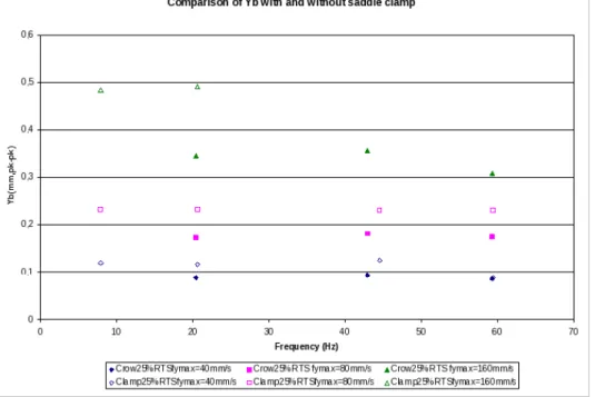
2.6 Influence of a suspension clamp on Yb measured near span end 39 2.7 Comparison between Yb at the suspension clamp and at the equipment clamp . . . 40
2.8 Conclusions . . . 42
3 Self-damping evaluated in actual conditions 45 3.1 Introduction . . . 45
3.2 Presentation of test equipment . . . 46
3.3 Self damping evaluated in actual conditions . . . 48
3.3.1 The self-damping power . . . 48
3.3.2 The wind power input . . . 49
3.3.3 Self damping fit with actual observations . . . 49
3.3.4 Wind power input comments . . . 52
3.3.5 Real world approach of power line vibration . . . 54
3.4 Conclusions . . . 54
4 The failure vibratory pattern of a conductor 57 4.1 Introduction . . . 57
4.2 Description of the set-up and tests . . . 57
4.2.1 The test span . . . 57
4.2.2 Conductors and fittings . . . 58
4.2.3 Test conditions . . . 58
4.2.4 Measurement of the conductor accelerations . . . 58
4.2.5 Measurement of the rotation of the conductor . . . 59
4.3 Analysis of the “noise” signal . . . 60
4.4 Failures . . . 64
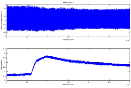
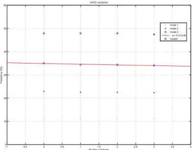
4.4.1 Failures of the AAAC conductor . . . 64
4.4.2 Failures of the ACSR conductor . . . 68
4.5 Detection of the failures . . . 70
4.5.1 Overview . . . 70
4.5.2 Eigen frequencies . . . 71
4.5.3 Tracking tools: wavelet transform versus short time Fourier transform . . . 74
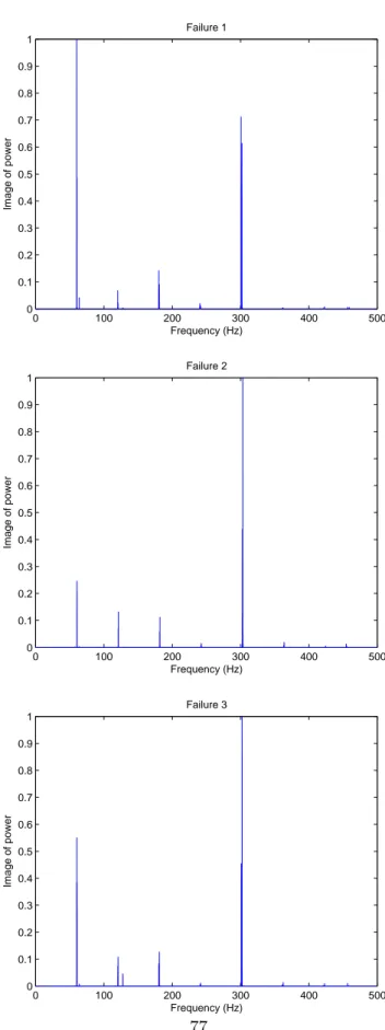
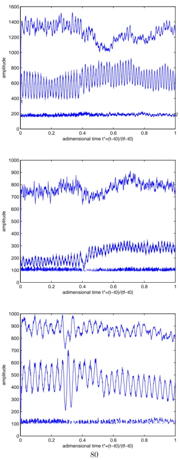
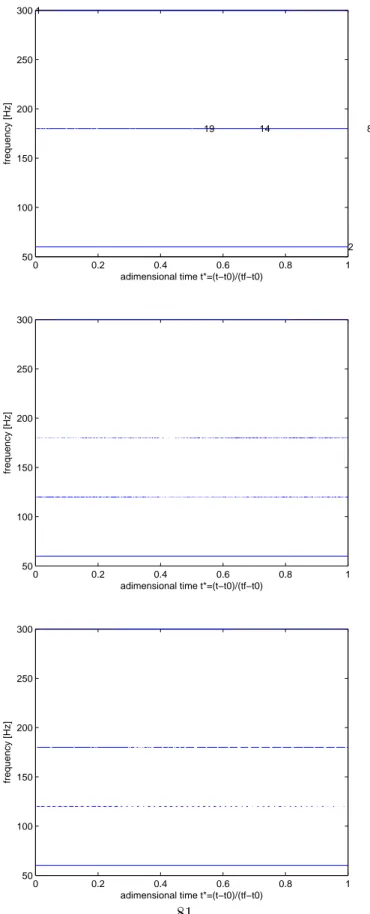
4.5.4 Study of the rotational acceleration . . . 76
4.7 Evolution of the eigen frequencies as the number of failures
increases . . . 86
4.8 Conclusions . . . 90
III Modelling 93 5 Basic model validation 95 5.1 Introduction . . . 95
5.2 Model description . . . 95
5.3 Shape of eigen modes . . . 96
5.4 Time response with a forced excitation . . . 98
5.5 Parametric study . . . 101
5.6 Reproduction of observed phenomena when in-span line equip-ment is introduced . . . 103
5.7 Time response . . . 106
5.8 Conclusions . . . 107
6 Tension fluctuations and related consequences 109 6.1 Introduction . . . 109
6.2 Equations for vertical motion . . . 109
6.3 Figuring the change in tension . . . 110
6.3.1 Simple formulation . . . 110
6.3.2 A more accurate formulation . . . 111
6.3.3 Comparison of the changes in tension computed ana-lytically versus with a finite element model . . . 111
6.4 Tension fluctuations in real spans versus laboratory test spans 115 6.4.1 Changes in tension in a single dead end span versus a section span . . . 115
6.4.2 The axial rigidity of span ends . . . 116
6.4.3 f ymax (amplitudes times frequency) and changes in tension in single dead end spans . . . 116
6.4.4 Checking the hypotheses made . . . 117
6.5 The effect of tension fluctuations on amplitudes . . . 118
6.5.1 Resolution of the constant tension problem . . . 118
6.5.2 Resolution of the variable tension problem . . . 124
6.5.3 Comparison of the variable tension problem without damping versus reality . . . 130
6.5.4 Comparison of the variable and constant tension prob-lems without damping . . . 132
6.5.5 Comparison of the variable and constant tension prob-lems versus reality when damping is introduced . . . . 133
7 Modelling conductor self-damping and bending stiffness 135
7.1 Introduction . . . 135
7.2 Relationship between curvature and moment versus conduc-tor bending stiffness . . . 136
7.3 The Available data collected by Godinas . . . 138
7.3.1 Presentation of the experiments . . . 138
7.3.2 Moment versus rotation angle curves . . . 138
7.4 Modelling strategy . . . 141
7.4.1 Introduction . . . 141
7.4.2 Viscoelastic model . . . 142
7.5 Deducing moment versus curvature curves from experimental measurements on conductor AMS621 . . . 142
7.5.1 Introduction . . . 142
7.5.2 Finite element model of the test-span . . . 143
7.5.3 The moment value of equation 7.4 . . . 144
7.5.4 How is the conductor tension affected by the tests? . . 145
7.5.5 From rotation angle to curvature . . . 145
7.5.6 The difference between rotation angle and curvature for a vibrating cable . . . 148
7.5.7 The dimensional homogeneity of the relationship be-tween moment and curvature . . . 148
7.6 Formula giving the power dissipated per unit length . . . 149
7.6.1 Introduction . . . 149
7.6.2 The area within the moment versus curvature curve . 149 7.6.3 Energy dissipated in a viscoelastic beam, under har-monic flexural loading . . . 150
7.6.4 Comparison of the self damping deduced from mo-ment versus curvature curves and other results of the empirical power law . . . 151
7.7 Deducing the viscoelastic model parameters from measurements153 7.7.1 Parameter A (which controls the slope of the hystere-sis curve) . . . 153
7.7.2 Parameter B (which controls the self damping via the area of the hysteresis curve) . . . 153
7.8 Dynamic bending stiffness deduced from measurements . . . 159
7.8.1 Slope of the moment versus curvature curve . . . 159
7.8.2 Comparison with K. Papailiou’s model . . . 160
7.9 Proposal of a new method for the measurement of a conduc-tor’s self damping properties . . . 161
7.10 The implementation of the viscoelastic model . . . 163
7.11 Another interpretation of the self-damping evaluated in ac-tual conditions (chapter 3) in light of the present conductor self damping model . . . 164
IV Model validation 169
8 Validation of the variable bending stiffness model 171
8.1 Average bending stiffness values deduced from measurements
on Ireq test span . . . 171
8.2 Comparison with other average bending stiffness values given in the literature . . . 173
8.3 Comparison with other variable bending stiffness models . . . 174
8.4 Conclusions . . . 174
9 Experimental attempts to reproduce resonance conditions 175 9.1 Introduction . . . 175
9.2 About the tests . . . 175
9.3 Phase shift between excitation force and conductor acceleration176 9.4 Excitation force . . . 181
9.5 Amplitudes at “nodes” of vibration . . . 183
9.6 Amplitudes at antinode of vibrations . . . 185
9.7 Conclusions . . . 187
10 Potential impact of the “non linear damping” in the energy balance 189 10.1 Introduction . . . 189
10.2 Energy injected within the beam . . . 190
10.3 Energy dissipated within the conductor . . . 190
10.4 Axial strain energy . . . 192
10.5 Conclusions . . . 192
V General Conclusions 195 11 General Conclusions 197 11.1 The new multi-tool strategy to assess conductor self damping 197 11.2 Understanding the impact of non-linearities . . . 198
11.3 Superiority of real on-site measurements . . . 199
11.4 Future work . . . 200
VI Appendixes 201 A Experimental moment versus rotation angle curves recorded by Godinas 203 A.1 AMS 621 . . . 203
B Dissection reports 209
B.1 AAAC conductor . . . 209
B.2 ACSR conductor . . . 211
C Calibration of the Hall sensors 213 C.1 AAAC conductor (testbench 6) . . . 213
C.2 ACSR conductor (testbench 3) . . . 214
D Data acquisition: matching between the accelerometer axes and the channels of the acquisition system 215 E Average bending stiffness of the AAAC conductor 217 F Self damping in mechanical systems 219 F.1 Introduction . . . 219 F.2 Material damping . . . 219 F.2.1 Viscoelastic damping . . . 219 F.2.2 Hysteretical damping . . . 220 F.3 Structural damping . . . 220 F.4 Fluid damping . . . 220 F.5 Viscous damping . . . 221
List of symbols
Symbol Description S.I. Unit
A Antinode single-peak amplitude of vibration [m]
A A = β(C⋆N )1/2−δ [kgm2/s2]
β Angle through which the conductor is bent
β Self damping parameter [kgm2/s2]
c Damping coefficient [N s/m2]
c Friction parameter (Coulomb model)
cm Mass proportional damping coefficient
ck Stiffness proportional damping coefficient
C Damping coefficient or matrix [N s/m]
CD Drag coefficient [1] C γ(C⋆N )δξ q EI N m D,d Diameter [m] D Damage parameter [1] D 2β(C⋆N )1/2−δ γ(C⋆N )δξ pEI N [kgm/s2] δr Reduced decrement ε Strain [1]
E Young’s modulus of elasticity [N/m2]
E∗ Parameter of the viscoelastic model [N s/m2]
E 2ymax(2πλ)2 [1/m]
f Frequency [Hz]
H Horizontal component of conductor tension [N ]
I Area moment of inertia [m4]
k Factor used in the power law
K Stiffness matrix [N/m]
l Exponent of the power law
L Span length [m]
L Length base quantity (Dimensional analysis)
λ Wave length [m]
Symbol Description S.I. Unit
M Mass matrix [kg]
M Mass base quantity (Dimensional analysis)
ml Conductor mass per unit length [kg/m]
m Exponent of the power law
µ Single-to-peak amplitude at the excitation point [m]
n Cycles of vibration
n Exponent of the power law
nwires Number of wires
N Number of cycles or number of samples
N Horizontal component of conductor tension [N ]
p qEIH [m−1]
P Power per unit length [W/m]
Φ Phase shift Re Reynolds number [1] ρ Density [kg/m3] St Strouhal number S Area [m2] Sc Scrouton number [1] σ Stress [N/m2] T Tension [N ]
T Time base quantity (Dimensional analysis)
v Speed [m/s]
W Work, energy [J]
w Weight per unit length [N/m]
ξ Coefficient [1]
y Vertical coordinate [m]
y0 Initial vertical coordinate [m]
ymax Antinode single-peak amplitude of vibration [m]
Yb or Yb2 Peak-to-peak bending amplitude [m]
measured at 89mm from the last point of contact between the conductor and the clamp
Yb1 Peak-to-peak amplitude measured at [m]
44.5mm from the last point of contact between the conductor and the clamp
Yb3 Peak-to-peak amplitude measured at [m]
178mm from the last point of contact between the conductor and the clamp
Acknowledgements
I acknowledge my principal advisor Professor Jean-Louis Lilien. During this thesis, I also received advice from Dr. Pierre Van Dyke, Professor Sylvain Goudreau and Professor Louis Cloutier. I acknowledge IREQ, Henri Pastorel and Dr. Pierre Van Dyke for allowing the use of their outstanding laboratory, Ireq’s members for their kindness and in particular the technical team who accompanied me during the tests: Roger Paquette, Martin Gravel and Jacques Poirier. I acknowledge GREMCA laboratory and their team for enabling me to collect remarkable fatigue material. I am grateful to University of Li`ege which has sponsored most of my travel costs through travel grants and my stay at University as assistant. Many thanks to the Ampacimon 3 team who made the “real outdoor tests” presented in the document possible. Last but not least, I acknowledge my husband and family for their unconditional support.
3Research project started at University of Li`ege in 2003 and initially sponsored by the French Community of Belgium
Introduction
The common thread of this document is aeolian vibration of overhead power lines. This phenomenon is characterized by vibration amplitudes of the or-der of the cable diameter and frequencies ranging approximately from 3 to 200 Hz [25]. The focus will be drawn to conductor fatigue4, in particu-lar to fatigue indicators, vibrational risk analysis, prediction of amplitudes, conductor self damping... No fluid aspect will be dealt with.
The input material for the study consists in several experimental mea-surements:
• Laboratory measurements performed at and supported by IREQ5,
• Continuous real outdoor span measurements performed by ULg using a new monitoring device developed at the same University, named “Ampacimon”,
• Laboratory measurements performed at GREMCA’s laboratory (Uni-versit´e Laval, Quebec),
• Original laboratory measurements made by A. Godinas at ULg on 4 meter long cable samples, which have not been exploited yet.
The analysis of these tests has led the author to propose a new non-linear model for overhead power line conductors, based on an existing non-linear beam finite element code and able to deal with both the variable bending stiffness and self damping properties of a conductor. Using a viscoelastic ma-terial with adequate parameter values, the moment versus curvature hystere-sis curves observed experimentally can be accurately reproduced (the area within the hysteresis represents the conductor self damping and the slope of the hysteresis its variable bending stiffness). All non-linear effects due e.g. to changes in tension are automatically coped with via the non-linearity of the finite element software itself.
4
The presence of aeolian vibration may result in another phenomenon called “fatigue of overhead conductors”. The latter being responsible for serious damage to overhead power lines.
5
This model will serve as a basis to interpret and discuss experimental re-sults. Some energy balances will also be produced in order to better quantify the different contributions to vibration amplitudes. Based on these devel-opments, a new formulation for conductor self damping will be proposed, which unlike others is based on the physics behind the phenomenon itself and is dimensionally correct.
Last, some new laboratory and on-site test ideas will be suggested in order to better assess the dynamic behaviour of conductors and hence their potential fatigue level.
Part I
Chapter 1
State of the art
1.1
When it all began
The first papers to address aeolian vibrations as a cause of fatigue of over-head lines were written in the beginning of the twentieth century. The Stockbridge damper, which is one of the first commercial devices to protect overhead lines against the harmful effect of vibrations, appeared around 1925. Lots of developments linked to fatigue have followed and are still ongoing, some of which are summarized in the next paragraphs.
1.2
Dangerous conditions and aeolian vibration
Dangerous conditions for conductor fatigue generally coincide with the pres-ence of Aeolian vibration. Fatigue may also occur from vibration phenomena called galloping or wake-induced vibration [25]. So-called Aeolian vibration on power line conductors is limited to low amplitude high frequency vortex shedding phenomena. Vortex shedding is characterized by vibration fre-quencies in the approximate range of 3-200 Hz and by amplitudes that can reach the conductor diameter for the lower range of frequencies [25].
As high frequencies are considered, it means that modal shapes have nu-merous loops along the span. All modes of a power line span have frequencies very close to each other, as the basic frequency is generally a fraction of Hz. Aeolian vibration can occur on almost any transmission line and at any time. Low turbulence wind will favour it [36]. Other parameters selected in [5] to qualify the vulnerability to Aeolian vibration are Hw, the ratio between the initial horizontal tensile load H and conductor weight per unit length w and also LDm , the ratio of the product of span length L and conductor di-ameter D to conductor mass m per unit length in the case of single damped conductors.
1.3
Fretting damage mechanisms
Dynamic stresses in a conductor are only partially due to bending. Since all wires are tensioned, it generates pressure on the layers below. This pressure results in friction during vibrations. At locations where the motion of the conductor is restricted, the curvatures are maximum and some micro-slip or even some sliding may occur. Due to the conductor cyclic motion, the direction of micro-slip is continually reversed, which may lead to the genera-tion of small cracks. Under small vibragenera-tion amplitudes, the contact pressure may stabilize them but under large amplitudes, some of them will further propagate and eventually cause a wire failure. Strand failures will occur where such singular conditions are created (where the conductor motion is restrained), mainly at suspension clamps but also at a damper, marker or spacer clamp [25]. Two fretting sub-cases are generally distinguished: fret-ting wear and fretfret-ting fatigue [48] but Waterhouse for example splits fatigue damage into three categories : fretting fatigue, fretting wear and fretting corrosion [89, 90]. According to [94], wording “fretting wear” must be used for surface movements induced by external vibration just as “fretting fa-tigue” must be related to surface movements induced by a cyclic loading of one of the two contacting parts. The development of long cracks is not re-stricted to fretting fatigue, but occurs also in fretting wear, as demonstrated by Vingsbo and Soderberg [88], Vincent et al. [87, 86, 93].
1.4
From friction between strands to damping
According to Hardy et al [38], most of the damping in the cable transversal motion comes from the friction between strands which takes place at the numerous wire contact interfaces. In other words, structural damping (de-fined in appendix F according to [80]) plays a preponderant role in cable self damping.
In 1985, Johnson derived an expression for the frictional dissipation per cycle when two materials are in contact [44]. Note that the sliding and therefore frictional damping between two materials in contact only occurs when a certain curvature level is reached (see e.g. [65]). Using this contact mechanics formulation as a basis, several authors have studied analytically the conductor self damping behaviour. In 1998, Goudreau et al [29] derived that the energy loss per vibration cycle is proportional to the cube of the vibration amplitude, inversely proportional to the tension in the cable and inversely proportional to the sixth power of wavelength. In 1999, Hardy et al highlighted the importance of flexural self damping in vibrations [38]. In 2008, Rawlins derived an expression of frictional dissipation at the contacts and extended it to a total dissipation per unit length of conductor [73]. The accuracy of the analytical self damping estimation is limited by the
hypothe-ses made and by the uncertainty associated to some input parameters such as friction coefficients, specific self damping capacity of a material at a given frequency, and also the tension in each wire (function of the load history and the composition of the cable).
1.5
Calculation of idealized stresses
The term “idealized stress” is used because the conductor fatigue mecha-nisms are so complex that the stress analysis has to be approximate. As an example, which value of bending stiffness should be used to perform a stress calculation? Also, it is difficult to deduce the stress state of a cable from measurement. Therefore, the alternating stress computed at the topmost fibre of a strand is generally chosen as an indicator of the stress state of a cable [25]. In 1936, Sturm published a paper where some simplified formulae to assess the stress in the vicinity of a clamp, and an analysis of the ways to reduce the maximum stresses were shown [82]. Other authors followed up with similar analyses ([58], [46], [76], [79], [12]). It is worth mentioning the formulae that give conductor curvature at the clamp:
• As a function of the angle through which the conductor is bent at the clamp by the vibration, β (see figure 1.1),
d2yt
dx2|x=0 = β
s H
EI (1.1)
• As a function of the antinode amplitude ymax
d2y t dx2|x=0 = 2π r m EIf ymax (1.2)
It is interesting to note that the conductor tension does not appear in the previous equation. This is due to the fact that the moment is the product of tension times its lever arm and that those two parameters vary in inverse proportion: the higher the tension, the sharper the conductor emerges from the clamp and the smaller the lever arm (see figure 1.1).
• As a function of the amplitude in the vicinity of the clamp d2yt dx2|x=0 = p2y e−px− 1 + px (1.3) p = s H EI (1.4)
Figure 1.1: Angle through which the conductor is bent at the clamp by the vibration, courtesy of EPRI [25]
This equation is well known as the Poffenberger-Swart formula [68]. The bending moment at the clamp can be obtained by multiplying the conductor curvature by EI. The stress is then obtained by σ = M vI (where v is half the diameter of the cable). Eventually, the formulae to compute idealized alternating stress in the top surface of a strand at the clamp are obtained [25]:
σa= dEa 2 β s H EI (1.5) σa= πdEa r m EIf ymax (1.6) σa= dEap 2 4 e−px− 1 + pxYb (1.7)
The industry standard position to measure y is at x=89mm (3.5 inches) [74] and, when measured at that position, its peak to peak value is called Bending amplitude (Yb = 2y).
In 1997, K.O. Papailiou published a paper where a new model for the variable bending stiffness of conductors is presented. In this model, interlayer friction and interlayer slip during bending are taken into account [65, 64].
1.6
Fatigue indicators
The residual life of a conductor is often determined as a function of some measure of vibration intensity [25]. The usual vibration intensity indicators are listed below:
• f ymax , the product of frequency by the free loop (antinode)
single-peak amplitude of vibration ([54, 1, 42, 81]),
• β, the angle through which the conductor is bent at the clamp by the vibration ([79, 7, 41]),
• Yb, the bending amplitude (amplitude of conductor relative to clamp,
measured a short distance, generally 89mm, from the last point of contact between the conductor and the clamp [83, 74, 45, 13]), • ε, the dynamic strain in an outer-layer strand in the vicinity of the
clamp, ([92, 59])
Fatigue curves have been developed through tests on laboratory spans using each of these parameters as the measure of vibration intensity.
According to [25], four problems arise in applying such fatigue curves in order to assess vibration of field spans.
• One is that (talking about f ymax, β, ε) “The parameter expressing
vi-bration intensity may be inconvenient to measure reliably in the field” and (talking about f ymax) “does not do justice to the complicated
behaviour found there”. Let us review those two arguments, with an engineer and pragmatic point of view. With a monitoring device able to measure the conductor accelerations, provided its position in the span is known, it should be possible to deduce f ymaxaccurately using
the wave propagation theory. Considering the second argument, it is true that f ymax does not reflect the interstrand fretting fatigue
mech-anism at the clamp, but indeed, which information is needed? An engineer who is in charge of the maintenance of transmission assets probably wants to know whether a line is at risk or not and whether remedial actions are needed. In this case, f ymax is an image of the
fatigue risk on a span. If in-span free-loop amplitudes are small, then the amplitudes in the vicinity of a clamped device will generally be small. The opposite is not true: the amplitude measured at a sus-pension span, where an armour rod may be installed, often behind a vibration damper will not necessarily reflect in-span amplitudes. Also, clamped devices will often be installed in-span (a spacer for example). Therefore, an analysis solely based on the measurement of Yb at the
span ends may fail to detect some vibration risks: Yb must therefore
• The second problem is that “vibration fatigue tests data are only avail-able for a small fraction of the conductor sizes and types that are in use, and such data are expensive to acquire. Since none of the above parameters is simply related to the fatigue-initiating stresses, results from tests on one conductor size are not necessarily applicable to oth-ers”.
• The third problem is that “fatigue tests have to be performed with a particular clamp” and it has been found that different types of clamps may yield to quite different fatigue test results.
• Finally, the fourth problem arises when field vibration amplitude is not a constant, “while available fatigue tests are performed keeping the selected amplitude parameter constant”.
1.7
Modelling of conductors and its limits
The models which are currently used to model aeolian vibrations are based on the energy balance principle, which states that “the steady-state ampli-tude of a conductor due to Aeolian vibration is that for which the energy dissipated by the conductor and other devices used for its support and pro-tection equals the energy input from the wind” [25]. The models based on this principle are simple, but are not able to take into account the reality, e.g. the excitation of several frequencies and the variation of wind in time and space. An improvement to the basic energy balance principle is to take into account a turbulent wind through a reduced wind power input [61, 19, 70]. However, this aspect of the problem has not been fully resolved yet and research is still going on. Research is ongoing also on more sophisticated models. These models can be either in time domain [18] or in frequency domain [61]. The target is to be able to model wind variation in space and time and to have a more realistic model of vortex shedding. There are still lots of work to do before those models are ready.
1.8
Usual check up
Most utilities, before stringing their lines or sometimes afterwards, face the difficulty of evaluating the vibration behaviour of a given power line. The difficulty mainly lies in choosing an appropriate stringing tension and eval-uating the number of dampers needed (or not needed) to prevent vibration damage and obtain an appropriate lifetime. In order to use the energy bal-ance principle, both a wind power input estimation and an estimation of the power dissipated by the conductor are needed. Conductor self damping and the wind power input are data very difficult to obtain (and indeed very strategic ones to evaluate lifetime based on calculations only). In absence
of data, literature provides values for wind power input and conductor self damping based on laboratory [25, 38], and wind tunnel testing [72]. In the past, it was both expensive and time consuming to perform tests in a labo-ratory or on a real span to collect representative information on conductor behaviour. In the coming years, the arrival of new commercial energetically autonomous vibration monitoring devices might make field measurements more common, accessible and easy. This should lead to more realistic stud-ies: actual conditions may be quite different from the cases observed in laboratory as long spans are used, fixtures are very different from one case to another and cable behaviour may vary significantly. An on-site mea-surement may give access to actual maximum amplitude for each of the frequencies after a certain time of observation (see chapter 3). On another side, the maximum observed amplitude may then be used to tune the en-ergy balance either thanks to the wind power input or the self damping (see section 3.3).
1.9
Non dimensional numbers related to self
damp-ing
Several authors commonly use the Scruton number in publications related to vibrations of cylindrical structures. This number is a dimensionless com-bination of variables and gives an image of the damping of the structure. Let us first define the following dimensional variables:
• ml, the cylinder mass per unit length [kg/m],
• ρ, the fluid density [kg/m3],
• d the cylinder diameter [m],
• C the system structural damping coefficient[N ∗ sec/m],
• Cc the cylinder system critical damping coefficient [N ∗ sec/m],
The mass ratio and the structural damping ratio, which are dimensionless variables, can be defined as:
m⋆= ml
ρd2 (1.8)
ζ = C Cc
(1.9) Let δ be the logarithmic decrement, which characterizes the free decay of a structure in time domain. In the field of overhead power lines, one can
write δ = 2πζ (see section 1.10.2). Then the Scruton number Sc can be defined as a combination of the two previous dimensionless variables:
Sc = δm⋆ (1.10)
Sc = 2πζm⋆ (1.11)
The Scruton number is therefore an image of the damping of the structure. It is often used in lieu of the reduced damping or reduced decrement
δr = 2mδ/(ρd2) (1.12)
1.10
Cable self damping measurement techniques
Different methods exist to measure conductor self-damping in laboratory: the power method, the inverse standing wave ratio, the decay method [25]. These are described in documents published by IEEE and EPRI [63, 25]. Self damping measurements are performed in laboratory test spans which length ranges from 30 to 90m. The conductor is held rigidly and strung at the required tension between two very stiff blocks. An electrodynamic shaker excites the conductor at one of its resonance frequencies. An example of such test span arrangement can be seen in figure 2.1.
These tests are carried out at different tension levels in order to account for the impact of tension on the interstrand friction zones. The results are corrected in order to subtract the self damping coming from the interaction between the vibrating cable and still air. Most of the time, these measure-ments are performed with the Inverse Standing Wave Ratio method (denoted ISWR), with which it is possible to separate the contribution of “in-span” and “span end” losses. Other methods are the power Method and the decay method. All three methods are described hereafter.
1.10.1 The power method
The power method states that the energy introduced in the span by the shaker is entirely dissipated within the conductor ([25], formula 2.3-9):
Win= Wdiss= πF µ sin(Φ) (1.13)
where Φ is the phase between the excitation force and the displacement, and F and µ represent the amplitudes of respectively the excitation force and displacement.
Note: formula 1.13 can be deduced from the general expression of external work given in chapter 13 of [56] : WE = R0∆Ftd∆t, where both Ft (the external force) and ∆t (the corresponding displacement) are a function of time. The integral value represents the area within the curve of force versus
displacement at the location of the excitation (both quantities are harmonic functions, with a phase shift equal to Φ) .
Let us assume the excitation corresponds to the kth eigen frequency of the span fk. The power dissipated per unit length of the cable is worth [25]
Pdiss= Wdiss
fk
L (1.14)
where L is the span length.
Let Wk,max be the maximum kinetic energy of the cable. Assuming a
modal decomposition of the vibration (with a single contribution from the excited mode), the position of the cable as a function of time y(x, t) satisfies:
y(x, t) = Aksin(
kπx
L ) cos(ωkt) (1.15)
where Ak is the single-peak antinode amplitude of vibration of the kth
mode.
The expression of the Wk,max is:
Wk,max= 1 2 Z L 0 mlω 2 kA2ksin2( kπx L )dx = 1 4mlω 2 kA2kL (1.16)
(which is identical to the expression of maximum kinetic energy given in [25], equation 2.3-11).
The damping is often expressed via the following non-dimensional damp-ing coefficient, also called “loss factor”(see [25], formula 2.3-10):
ζk=
Wk,diss
4πWk,max
(1.17) Applying the power method, one must keep in mind that extraneous dissipation sources (e.g. external sources of damping and end damping) are included in the measurements [25].
1.10.2 The decay method
In the decay method, the cable is forced to vibrate at one of its eigen fre-quencies, the kth one for example. Then the excitation is stopped and the
decay of the cable studied [25]. If Xk,iis the amplitude of motion during the
decay cycle i (the abscissa where Xk,i is measured does not really matter,
provided the measurement is performed at the sample place from one cycle to another), the logarithmic decrement δk is defined as δk = ln(XXk,i+1k,i ). If
of magnitude of 10−3), the non dimensional damping coefficient is simply
given by ([25]):
ζk=
δk
2π (1.18)
This second method requires the excitation to be stopped properly so that the shaker is perfectly disconnected from the cable and that no un-wanted impulse is induced [25]. It also has the disadvantage of including extraneous losses like end damping in the measurements.
1.10.3 The ISWR method
The third method, called ISWR requires the amplitudes of vibration at some nodes to be measured as well as an amplitude at an antinode. The method is derived from the work of Tompkins et al [85] and is based on the principle that if there were no dissipation within the cable, no motion at nodes would occur (because incident and reflecting waves are equal). The motion that occurs at vibration“nodes” hence reflects the damping within the conductor. The amplitudes at vibration “nodes” are small (a few micrometers), which makes their measurement difficult. Let us suppose the span is vibrating at its kth eigen mode. Let us define the inverse standing wave ratio as
Sk,i=
ak,i
Ak
(1.19) where ak,iis the single amplitude of vibration in a node and Akthat at a
vibration antinode. From an electromechanical analogy, Tompkins derived that the power flowing through one section of a cable is given by [85]:
Pk,i= V2 k 2 Sk,i p T ml (1.20) with Vk= ωkAk
The power dissipated between nodes i and j distant of nv half-wave
lengths is equal to
Pk = Pk,i− Pk,j (1.21)
The power dissipated per unit length of the conductor is then
Pk,diss =
Pk,i− Pk,j
nvλk/2
(1.22) From the definition of the maximum kinetic energy of a cable on the one hand and the expression of frequencies of a string, it can be deduced that the non dimensional self damping coefficient ζk is given by:
ζk=
Sk,i− Sk,j
nvπ
(1.23) Provided the amplitudes of vibration at nodes can be measured ade-quately, the ISWR method permits to withdraw the contribution of span ends and external devices and to consider only the energy dissipation which takes place within the portion of cable under study only.
1.11
Experimental self damping power law and
similarity law
The power dissipated per unit length of conductor is often expressed empir-ically through a power law:
Pdiss= k
yl
maxfm
Tn (1.24)
Where Pdiss is the self damping power per unit length [W/m], k is a
proportionality factor depending on cable data, ymax is the antinode zero to
peak amplitude [m], f the frequency [Hz] and T the tension in the conductor [kN]. The exponents l, m, n may vary significantly but are generally in the range given in table 1.1. Let d [mm] and RTS [kN] be respectively the conductor diameter [mm] and RTS its rated tensile strength [kN]. The k factor satisfies
k = p d[mm]
RT S[kN ] ∗ mL[kg/m]
(1.25) and is close to 1.5 or 2 for classical conductor material and cross section in SI system [24]. In 1998, a Cigr´e working group collected information on the coefficient found experimentally by different laboratories around the world [84].
Table 1.1: Range of the exponents l, m, n of the self damping power law Factor Range
l 2-2.5
m 4-6
n 2-2.8
k 1.5-2
In [25], the following interesting comment is given: the exponents vary significantly according to the measurement method and the configuration of
span ends. When the power method is used with span ends rigidly fixed, the amplitude exponent is close to 2 and the frequency exponent close to 4. When the ISWR or the power method with pivoted extremities is used, the amplitude and frequency exponents are close to respectively 2.4-2.5 and 5.5. Reminding the discussion of the previous paragraph, this difference is mainly due to span end effects, which can not be withdrawn in the power method with rigidly fixed ends. Self damping coefficients deduced from the ISWR method and power method with pivoted ends therefore give a more accurate value of the self damping which comes exclusively from the conductor.
A comparison of the self damping power computed using coefficients deduced with the same method (ISWR), but by different authors will be shown in chapter 3, section 3.1. It shows important scattering within the results (the self damping values may differ by one order of magnitude).
As mentioned in the previous paragraph, the self damping characteristics of a conductor will depend among others on the wire material (e.g. for a given size and topology, the damping behaviour of an ACSR conductor will be very different from an aluminium alloy conductor), and on the size of the friction zones (and therefore on the size of the conductor and its amount of layers). Self damping power laws are therefore established for one given conductor, characterized by its material, number of wires, mass per unit length... Since the tests required are expensive, one author has studied the possibility to extrapolate the self damping laws to other conductors from the same class and with a similar size. In 1997, Noiseux published generalized similarity laws for near-field (near span ends) and free field (in span) loss factors for ACSR conductors. Once self damping measurements have been performed on a given ACSR conductor, these similarity laws permit to predict self damping for other ACSR conductors with identical constructions but different diameters [62].
1.12
The wind power input
Wind power input data is based on wind tunnel experiments made in the air flow at different reduced velocities. Curves of power as a function of ymax/d (single-peak amplitude/diameter ratio, denoted A/d in [25] and the
following figure) are then drawn from these test data. The maximum energy input curve is finally determined by the envelope of all the curves.
The tests to evaluate the maximum energy input are made on rigid or flexible cylinders, leading to different results, as can be seen in the following figure. The curves representing the flexible cylinder tests are in [70, 8], while others represent the rigid cylinder tests.
There are several characteristics of wind power input and of the method used to obtain relative curves which are worth being mentioned in the present report. The initiation of aeolian vibrations occurs when the
ve-Figure 1.2: Wind power input curves measured for different reduced velocities, courtesy from EPRI (A is the peak-to-peak displacement/2) [25]
Figure 1.3: Maximum wind power input coefficient in case of a single conductor, A is the peak-to-peak displacement (courtesy from[25], based on [8])
locity of the incoming flow is such that the frequency of the vortices shed in the wake of the conductor approaches a modal frequency of the span. Such a velocity is called onset velocity in the literature [25]. The shedding frequency of the vortices is given by the following relationship:
fst=
Stv
d (1.26)
where St is the Strouhal number, v is the fluid speed [m/s] and d the
diameter of the cylinder which is plunged into the flow [m]. The Strouhal number may be function of three criteria:
• the Reynolds number (Re)1 • the relative surface roughness, • the aspect ratio.
The effect of the two latter criteria can be considered as small for overhead conductors. Thus the vortex shedding phenomenon can be considered as “governed” by two non-dimensional numbers: the Strouhal number and the Reynolds number. In the range of Reynold’s number of interest for aeolian vibrations (350 < Re < 35000), the value of the Strouhal number is almost constant and approximately equal to 0.18 [25]. Once aeolian vibrations are installed, in other words for larger amplitudes of vibrations, the vortex shedding frequency may be “locked” by the vibration of the cylinder and aeolian vibration may continue to exist even if the velocity of the incoming flow is slightly changed. Experimentally, it was possible to maintain aeolian vibrations with wind velocities comprised between 90% and 130% of the onset velocity. This phenomenon is called lock-in and has an impact on the method used to deduce wind power input curves. In order to plot wind power input curves, several reduced velocities2 are considered. Only the maximum values obtained for different reduced velocities are eventually retained to plot wind power input curves. Also, both the oscillation amplitudes and the wind power input show a hysteresis: depending on the initial conditions of excitation, the wake flow pattern can either be a 2P or 2S mode3 which results in two branches in the wind power input curves [8].
The turbulence of the incoming flow is another parameter which will influence the value of the power imparted by wind to a vibrating conductor. The lower the turbulence, the higher the wind power that can be imparted
1
Let v be the flow velocity [m/s], ν the kinematic viscosity of the fluid (m2
/s) and d the conductor diameter [m]. The Reynold’s number is given by the ratio V d
ν . 2
a reduced velocity is the ratio of flow velocity on the Strouhal onset velocity 3
The name of the shedding mode “2P” or “2S” comes from the pattern in the wake of the conductor which can be characterized either by the shedding of two pairs of vortices (2P mode) or two single vortices (2S mode) per cycle of oscillation
to the conductor. Rawlins has published a paper where a model is proposed in order to take into account the turbulence of wind [72].
1.13
Analysis of a span with (a) damper(s)
In 2005, Cigr´e working group 11 issued a report on Modelling of aeolian vibration of a single conductor plus damper [4]. Other useful information on this topic may be found in [25]. The question which needs to be answered by grid owners is the following: “How much damping needs to be introduced in the overhead power lines in order to keep them safe from vibration damage”. To answer this question, several approaches are described in the literature, depending on the possibility to feed the analysis with experimental data. The first step of the procedure is to assess the damping efficiency of the cable plus damper system. Here is how this first step is performed:
• If the damper can not be tested, the first step is to build a model of this equipment. Then the mode shapes of the span plus damper system need to be computed so that a modal solution for the equation of motion can be sought.
• If the frequency response of the vibration damper is known (e.g. if a test on a vibration shaker has already been performed), this input can be introduced in the span model under the form of an equivalent transmitted force. In such a case, the model must be able to simulate the span distortion caused by the damper presence,
• If it is possible to perform self damping laboratory tests of the ca-ble+damper system, then the power dissipated by the damper will be measured at different frequencies of interest for aeolian vibrations and at different amplitudes.
Then, the second step is to estimate the vibration amplitudes which can be expected on-site. Once again, field recordings will provide the most appropriate and complete answer to this question. In their absence, the amplitudes will be estimated thanks to the Energy Balance Principle EBP. The wind power input information can be either modelled (e.g. using [72]), or (advantageously) measured on-site.
The last step is to perform a vibration risk diagnosis. In case the inci-dence level of fatigue is unacceptable, more damping needs to be introduced and the analysis restarted.
C.B. Rawlins has investigated the vibration damping on long spans [69], characterized by non sine shaped modes and variable loop amplitude along the span. His conclusions mention that the effect of the great length of the span is to reduce the amount of damping needed by 10 % for overland spans and by 25% for span crossings.
1.14
Cigr´
e recommendations
In 1950, a first report was presented by the members of the group “Cigr´e Comit´e d’´etudes 6” [16]. The conclusion of this first report was that an adequate conception of clamps should prevent vibration damage. Ten years later, another report was published, based on the statistical analysis of the conductor mechanical tension [17]. The concept of Everyday Stress (EDS) was introduced, which is the stress in the conductor, expressed as a percent-age of its tensile strength, at his averpercent-age temperature and without (mechan-ical) overload. A maximum EDS was recommended. Nevertheless, failures happened even if the EDS value was very low, e.g. < 15%. This is due to the fact that fatigue depends on several other parameters than EDS (topog-raphy, turbulence of wind, type of clamps, manufacturing of the line). Cigr´e researches posterior to 1960 (mainly those based on conductor self damp-ing) have shown that the ratio of horizontal tension load and the conductor weight per unit length (H/w) was probably a more appropriate parameter than EDS. In 2005, Cigr´e 22.1, TF4 recommended the H/w values present in figure 1.4 [5].
Figure 1.4: Recommended Safe Design H/w values for single unprotected conductors, Cigr´e 22.11 TF4 2005
For damped single conductor, the same working group proposes a new parameter for rating the protective capabilities of dampers [4]. This pa-rameter is √LD
Hm(L is the span length, D the conductor diameter, H the
horizontal tension and m the mass of conductor per unit length). Since
H
w is a commonly used parameter, Cigr´e then decided to simplify the two
parameters √LD
Hm and H/m in Ld
m and H/w. Figure 1.5 shows the design
recommendations of Cigr´e working group 22.11, TF4, 2005. Four sets of curves are presented. Each one is associated to a certain type of terrain category described in the legend.
Figure 1.5: Recommended safe design tension for single conductor lines. H: initial hori-zontal tension; w: conductor weight per unit length, L: actual span length, D: Conductor diameter and m: conductor mass per unit length [5].
1.15
Vibration recorders
Most existing vibration recorders try to measure the bending amplitude of conductors. Vibration recorders designed to measure antinode amplitude are quite recent.
Let us first review the bending amplitude recorders. The oldest bend-ing amplitude recorders are analog devices such as Ontario Hydro recorder (1963). Those devices, developed by Edwards and Boyd [22] contained a clock and were timed to obtain one second recording every 15 minutes. The autonomy of this instrument was about 3 weeks and it was necessary to take it off the line to get the recorded data. Other analog bending ampli-tude recorders are HILDA and Sistemel.
Digital recorders are micro-processor based, battery-powered, with a memory in which the data are stored under a digital form. Examples of such devices are Vibrec, Pavica, Scolar III and Ribe LVR vibration recorder. The autonomy of these devices is of the order of a few months. The weight of these instruments ranges from 0.5kg (Pavica) to 3.1kg for Scolar III ( but 6.1kg with standard fittings) [3]. Since these devices are battery powered, in order to spare energy, these devices are only able to perform intermit-tent measurements. According to [3], Scolar III can be set up for 1 to 4 seconds every 10 minutes and in general, vibration recorders perform ten seconds recordings every fifteen minutes. Then, the recorders have to per-form a data reduction because of storage limitations. The frequency and the amplitude of the vibration cycles are measured by suitable algorithms and stored in a memory matrix according to the procedure suggested by IEEE [74]. The Pavica and Scolar III recorders store the highest amplitude and the average frequency of any sample period. Other recorders like Vibrec400 and Ribe LVR store amplitude and frequency of each individual cycle recorder in the sample period. In paper [3], U. Cosmai stresses that the results ob-tained with these two procedures can be rather different. In the frame of this thesis, it is also stressed that lots of information is lost when vibrations are recorded only for a few seconds every 10-15 minutes. The occurrence of vibration at a given location is far from obvious. In 2003, University of Li`ege started a project (named Ampacimon) with the aim to conceive a vibration monitoring device. The particularity of this device is that for the first time, the device is installed in-span, is energetically autonomous and is able to perform continuous vibration measurement.
1.16
Fatigue curves obtained in laboratory
Fatigue curves are generally established relative to f ymax or to bending
amplitude. The idealized dynamic stress can be calculated using equation (1.)6 or (1.7). Examples of such fatigue curves drawn at constant amplitude
with conductors supported by rigid ends can be found in [25]. Let us consider fatigue curves relative to f ymax. One of these is shown in figure (1.6),
relative to f ymax. Most data used to plot these figures come from Alcoa
and Gremca laboratories.
Figure 1.6: Fatigue tests of three-layer ACSR, courtesy from EPRI [EPRI2006]. The number of cycles N leading to a first strand failure at a given ampli-tude shows a wide scattering rather than a “well defined fatigue curve” [25] (chapter 3). Having examined several of those fatigue curves, the authors of that chapter noticed that:
• Given a conductor and its supporting clamp, the level of tension in the conductor seems to have little effect on the fatigue curve,
• Given a conductor and its supporting clamp, the number of layers appears to have some influence on the fatigue curve,
• The σa-N relationship is relatively insensitive to clamp contour.
In case there is no S-N (stress S depending on the number N of cycles to failure) available for a certain conductor, the Cigr´e safe border line can be used. This curve is derived from various laboratory fatigue measurements. It represents the conservative lower limit of the permissible number of cy-cles at various stress levels. It is applicable for commonly used aluminium, aluminium alloy and multi-layer ACSR conductors and all types of clamps. The safe border line can be seen in figure 1.7 and is represented by the following equation:
σbf = CNz (1.27)
where σbf is the dynamic limit stress in N/mm2, N the number of cycles
until failure, C = 450 and z = −0.2 for N ≤ 2 ∗ 107 and C = 263 and
z = −0.17 for N ≥ 2 ∗ 107 [91].
Figure 1.7: Cigr´e safe border line
1.17
Cumulated damage from constant amplitude
to variable amplitude and frequency
As explained in the previous section, fatigue curves are drawn from lab-oratory tests, considering constant amplitude of vibration. In reality, the conductor will undergo variable amplitudes of vibration. To go from the constant to variable amplitude situation, the usual approach is to consider a “cumulated damage law”. One of the simplest cumulated damage law is the Palmgren-Miner one, often denoted Miner’s law. Assuming a conductor specimen to be subjected to k stress amplitude levels σi, this rule consists
in calculating an equivalent damage parameter D as follows [57, 39]:
D = k X i=1 ni Ni (1.28) Where
• ni is the number of cycles at stress amplitude i,
• Ni is the number of cycles to failure if the specimen was subjected to
constant amplitude level i.
According to Miner’s rule, the failure occurs for D = Df = 1 (Df is the
damage at failure). Nevertheless, one should be aware that Miner’s law has two limitations, which have been proven by tests [77]:
• The sequence of occurrence of amplitudes (i.e.: the load history) is not taken into account in the previous law,
• The impact of amplitudes below the endurance limit is not taken into account (for N approaching infinity).
Improvements to this damage law have been proposed in [77], but Miner’s rule still remains used because of its simplicity. Its validity for conductor fatigue has been tested to some extent (see for example [30, 31]). In [10], a study of the value of the damage parameter is reported. It appears that Df is not a constant but rather follows a statistical distribution and extends
over at least a 3:1 range. The use of Miner’s law has been recommended by Cigr´e, but with the remark that the critical value of Df (damage at failure)
may vary from 0.5 to 2. If D = 0.5, life time is divided by 2 compared to D = 1, and if D = 2, life time is multiplied by 2 compared to D = 1.
1.18
Estimation of conductor lifetime
In [47], one can find a complete description and an example of the procedure to assess a conductor lifetime. This procedure comprises uncertainties and approximations.
First, if the “load history” comes from an old type of vibration recorder, as explained in the paragraph devoted to these devices, because of energy savings, these devices only perform a few seconds of vibration measurements every 10 to 15 minutes. Out of these few seconds of records, one amplitude is saved in memory. Lots of information may then be lost on the real “load history”. The recordings may not represent the real conditions. With new energetically autonomous devices, continuous measurement is possible [53]. Second, as mentioned by [20], the local terrain affects the severity of vibration. Even if there has been no systematic study of the variability of vibration severity structure-to-structure in any line, the exposure to fatigue probably varies span-to-span. Choosing a single test structure means taking a single sample out of a population of structures having varied exposure to damage. This should be taken into account when doing a fatigue analysis.
Third, it has also been shown by [23] that the behaviour of the different phases at the same tower can be different.
In the fourth place, the severity of vibration varies with weather condi-tions, on an hourly and daily basis and as seasons go by [67]. A full year of record should be preferred to account for these seasonal effects [20].
In the fifth place, the recorder, by its presence, can change the variable that is being recorded. The mass of the instrument alters the inertial prop-erties of the support where it is attached. In some cases, a resonance can occur that results in amplification of amplitudes at some frequencies and reduction at others [78, 11, 34, 40].
In the sixth place, the intensity of vibration displays variations in the form of beats. This beating pattern exists because more than one vibration mode may be excited at the same time. All these aspects complicate the problem of interpreting recorded data by means of laboratory data on the fatigue characteristics of conductors [20].
Last, as mentioned in one of the previous sections, fatigue curves are obtained with tests run at constant amplitude. The problem is convention-ally dealt with through Miner’s rule which also has its limitations: both the sequence of occurrence of amplitudes and amplitudes under the endurance limit are not taken into account (see section 1.13). Moreover, the parameter of damage at failure is not a constant and extends over a at least a 3:1 range. For all these reasons, estimation of conductor lifetime is an extremely challenging task.
Part II
Chapter 2
Evaluation of power line
cable fatigue parameters
based on measurements on a
laboratory cable test span
2.1
Introduction
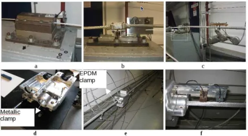
The present chapter describes experiments carried out on IREQ’s1 labora-tory cable test bench by Suzanne Gu´erard (ULg), Roger Paquette, Martin Gravel and Jacques Poirier (IREQ), under the supervision of Pierre Van Dyke (IREQ). Test span arrangement is a 63.15m cable span with termi-nation ends designed to minimize energy dissipation. A shaker provides a vertical alternating force to the conductor. During the experiments, a maximum of information on mode shape is collected: location of nodes, antinodes, relative displacement at 44.5, 89, and 178mm from the last point of contact with the metallic clamp. Several configurations are studied: span equipped with a homogeneous steel cable, span equipped with an ACSR 2 Crow conductor, sometimes in combination with other equipments such as a vibration damper or a local mass, to investigate how the presence of such devices impacts conductor vibrations. It results from these experiments an interesting comparison of two widely used fatigue indicators, the relative dis-placement Yb (also called “bending amplitude”)3 and f ymax (the product
1
IREQ: Institut de Recherche d’ Hydro-Qu´ebec, www.Ireq.ca 2
Aluminium Conductor Steel Reinforced 3
Peak-to-peak displacement of conductor relative to the clamp, generally measured at 89mm from the last point of contact between the conductor and the metallic clamp. In this chapter, Yb1, Yb2 (= Yb) and Yb3stand for relative displacement measured respectively at 44.5, 89 and 178mm from the last point of contact between the conductor and the metallic clamp
of antinode amplitude of vibration by frequency).
Recognized vibration intensity indicators are the product of antinode amplitude of vibration by frequency (f ymax) [1, 7, 13], angle through which
the conductor is bent at the clamp [42, 74, 45], relative displacement (Yb) [59,
79, 81] and dynamic strain at the surface of an outer-layer strand (usually measured at the top of conductor [43]) in the vicinity of the clamp [83, 92]. Fatigue curves may be obtained through tests on laboratory spans using any of those parameters as the measure of vibration intensity, but it is more common to see fatigue curves drawn as a function of relative displacement, f ymax or an equivalent idealized stress [25].
Among those vibration intensity indicators, relative displacement has been used for field measurement for decades [74]. However, nowadays, new technologies are being developed, which allow continuous antinode ampli-tude monitoring. Given this context, it is interesting to investigate what are the opportunities associated with real time field measurement of antin-ode amplitude of vibration, in order to perform a vibration risk diagnosis of a line. The tests performed on IREQ test span allow to compare rela-tive displacement and f ymax as vibration intensity indicators and to bring
interesting arguments in this discussion.
The tests performed also meet the following objectives:
• Collect all the required data to validate the modelling of a conductor vibrating at its natural vibration modes,
• Improve the understanding of conductor behaviour at singularities along the span where the impact of conductor bending stiffness is particularly important. Examples of such singularities are suspension clamps, spacer (damper)/damper clamps, aerial warning markers, real time monitoring devices, etc..
• Improve the understanding of the interaction between parameters Yb
and f ymax,
• Finally, collected data also enables the assessment of conductor self damping.
2.2
Presentation of test equipment
A sketch of IREQ 63.15m long laboratory test span is shown in the figure 2.1. The conductor is installed into rigid clamps which are part of an extremely stiff concrete block embedded in the rock underground in order to minimize end losses. Conductors are tensioned at least 24h before the beginning of tests, in order to get a final tension value of approximately either 15 or 25% of their RTS (rated tensile strength). An electrodynamic shaker located at
![Figure 1.6: Fatigue tests of three-layer ACSR, courtesy from EPRI [EPRI2006].](https://thumb-eu.123doks.com/thumbv2/123doknet/6781640.188002/43.918.194.654.218.539/figure-fatigue-tests-layer-acsr-courtesy-epri-epri.webp)