HAL Id: hal-00433600
https://hal.archives-ouvertes.fr/hal-00433600
Preprint submitted on 20 Nov 2009
HAL is a multi-disciplinary open access
archive for the deposit and dissemination of
sci-entific research documents, whether they are
pub-lished or not. The documents may come from
teaching and research institutions in France or
abroad, or from public or private research centers.
L’archive ouverte pluridisciplinaire HAL, est
destinée au dépôt et à la diffusion de documents
scientifiques de niveau recherche, publiés ou non,
émanant des établissements d’enseignement et de
recherche français ou étrangers, des laboratoires
publics ou privés.
Markov Aspect Models
Wen Yang, Dengxin Dai, Bill Triggs, Gui-Song Xia
To cite this version:
Wen Yang, Dengxin Dai, Bill Triggs, Gui-Song Xia. Semantic Labeling of SAR Images with
Hierar-chical Markov Aspect Models. 2009. �hal-00433600�
Semantic Labeling of SAR Images with
Hierarchical Markov Aspect Models
Wen Yang, Dengxin Dai, Bill Triggs, Gui-Song Xia
Abstract—Scene segmentation and semantic labeling of
Syn-thetic Aperture Radar (SAR) images is one of the key problems in interpreting SAR data. In this paper, a new approach for semantic labeling of SAR imagery is proposed based on hier-archical Markov aspect model (HMAM) with weak supervision. The motivation for this work is to incorporate the multiscale spatial relation between adjacent image patches into supervised semantic labeling of large high resolution SAR image. Firstly, the large SAR image is divided into hundreds of subimages, and the semantic keywords of each training subimage are given by the user. Then, the HMAM is presented by building markov aspect model based on quadtree which can explore multi-scale cues, spatial coherence and thematic coherence simultaneously. Next, we use the trained HMAM model to classify each patch of the unlabeled subimages into a given semantic classes. Finally, we regroup all the labeled subimages into the large SAR scene labeling result. We also elaborately build the ground truth map for a whole scene of TerraSAR-X image to evaluate the labeling results quantitatively. The experimental results on TerraSAR-X dataset show that our labeling method is effective and efficient, and the HMAM can improve labeling performance significantly with only a modest increase in learning and inference complexity than aspect model.
Index Terms—Synthetic Aperture radar (SAR), Image labeling,
Hierarchical markov aspect model, Probabilistic latent semantic analysis (PLSA).
I. INTRODUCTION
Over the last decade we have witnessed an explosion in the number and throughput of airborne and spaceborne SAR imaging sensors. At the same time, advance in data transmission and store have made it increasingly possible to acquire and order SAR image data at a relative lower cost. The evergrowing large volumes of SAR images place a heavy demand on providing an effective and efficient image analyzing method for understanding SAR imagery. In this work, we are interested in semantic labeling of a large SAR image with weak supervision, which is aimed at partitioning a SAR image into their constituent semantic-level regions and assign appropriate class label to each region. SAR image labeling has several additional difficulties. Firstly, SAR image suffers from a noise-like phenomenon known as speckle which results in large variation of the backscatter across neighbor-ing pixels within a sneighbor-ingle distributed target, even in a flat region, such as the road surface. Secondly, a scene of SAR
W. Yang and D.X. Dai are with the Signal Processing Lab, School of Electronics Information, Wuhan University, Wuhan, 430079 China e-mail: yangwen94111@yahoo.com.cn; ddx2004@gmail.com.
B. Triggs is with Laboratoire Jean Kuntzmann, B.P. 53, 38041 Grenoble Cedex 9, France e-mail: Bill.Triggs@imag.fr
G.-S. Xia is with CNRS LTCI, Institut Telecom, TELECOM ParisTech, 46 rue Barrault, 75634, Paris Cedex-13, France, e-mail: xia@enst.fr
image is usually very large, which poses a higher efficiency requirement to image labeling algorithm. Thirdly, researchers unable to validate their ideas adequately because there is no a publicly available SAR imagery labeling ground truth dataset. Finally, this task is still challenging because of the well-known “aperture problem” of local ambiguity. For example, a homogenous dark region in SAR image maybe a piece of calm water, radar shadow, or road surface. Fig.1 shows two similarly dark regions. These two patches are not easily distinguishable without using context cues. Actually, one of them is the radar shadow owning to obscuration by the buildings within the illuminating radar beam, the other is water surface.
Statistical distribution models with the maximum likelihood classification methods are well known and widely used in SAR image segmentation and classification. However, they are usually pixel-based methods which cannot handle the abundant information of SAR imagery and produce a characteristic and inconsistent salt-and-pepper labeling map. Many works built their models on Markov random field (MRF) to involve spatial relationship, often with remarkable improvement. Venkatacha-lam et al. [1] applied the wavelet-domain Hidden Markov Tree (HMT) models as a reliable initial segmentation, and then refined the classification using a multiscale fusion technique. Tison et al. [2] proposed a classification method based on Markovian modeling that uses a new statistical model with the Fisher function, which is suitable for high-resolution SAR images over urban areas. Deng et al. [3] used a function-based parameter to weight the two components in a MRF model and produced accurate unsupervised segmentation results for SAR sea ice images. For further reduce the impacts of speckle on classification performance with the pixel-based methods, many region-based methods had been proposed. Yang et al. [4] pro-posed a region-determined hierarchical MRF model for SAR image classification based on watershed over-segmentation algorithm, and demonstrated better results than the pixel-based hierarchical MRF model. Xia et al. [5] presented a precise segmentation of SAR images using MRF model on region adjacency graph (MRF-RAG), and a rapid clustering method for SAR image segmentation was further proposed in [6], which embedded a MRF model in the clustering space and used graph cuts for optimization. Wu et al. [7] proposed a region-based classification method for polarimetric SAR images using a Wishart MRF (WMRF) model to overcome the isolated pixels and small regions in classification maps using pixel-based methods due to speckle in polarimetric SAR images. However, These works only tested their methods on small SAR images and most of them had not yet listed their quantitative results.
Supervised SAR image classification using advanced clas-sifiers originally arise from machine learning domain has shown exceptional growth in recent years, such as neural networks [8][9] adaboost [10][11], Support vector machine (SVM) [12][9] and random forests [13]. These methods can handle limited training samples and usually achieve the state of the art labeling performance. However, training samples with pixel-level detailed labeling are still necessary for using these methods.
Recently, many research works on labeling natural images focus on the utilization of high-level semantic representation and informative context information, such as the Probabilistic Latent Semantic Analysis (PLSA) [14] or its bayesian form, the Latent Dirichlet Allocation (LDA) [15]. They consider visual words as generated from latent aspects (or topics) and expresses images as combinations of specific distributions of topics, which are well appropriate to the semantic labeling task by capturing thematic coherence (image-wide correlations) and can resolve some cases of visual “polysemy”. Li´enou et al. [16] proposed to exploit the LDA model to semantically annotate large high-resolution satellite images. The experi-mental results on panchromatic QuickBird images with 60-cm resolution demonstrated that using simple features such as mean and standard deviation for the LDA-image representation can lead to satisfying labeling results. However, as a model proposed for document analysis, aspect model has its own limitation on image labeling. Firstly, there are no apparent vi-sual words in image. Researchers often obtain vivi-sual words by clustering the features extracted from image patches at a single scale which leads to failure in capturing the instinct multi-scale cues in image. Moreover, aspect models assume that the labels of adjacent patches are independent, thus ignoring the strong correlations that are found in real image. Verbeek and Triggs [17] developed two spatial extensions of PLSA, but multi-scale cues were not considered. Cao et al. [18] used Latent Dirichlet Allocation at the region level to perform segmentation and classification and enforce the pixels within a homogeneous region to share the same latent topic. There are also some more complicated topic models, such as Harmonium model based on undirected graphical models [19], Pachinko Allocation Model based on directed acyclic graph [20], and their variants. However, these models all need the sophisticate parameter estimation and model inferencing algorithm.
In this paper, our goal is to design an effective and efficient labeling algorithm which can handle the semantic labeling of large-scale SAR images. We develop a further extension of markov aspect model-HMAM, based on quadtree which can explore multi-scale cues, spatial coherence and thematic coherence simultaneously. The later experimental results will demonstrate the priority of our method. The contributions are threefold: Firstly, an efficient SAR images labeling method based on aspect model is introduced which only needs keywords-labeled training samples, as shown in Fig.2). It avoids the labor-intensive and time-consuming work to label every pixel in SAR images for obtaining detailed pixel-level training data. Secondly, we propose a hierarchical Markov aspect model (HMAM) based on quadtree which can fully exploit the multiscale spatial context information; Thirdly, we
build a whole scene TerraSAR-X image ground truth map, with which practitioners can evaluate their labeling algorithms quantitatively.
Fig. 1: Top: two ambiguous image patches and their his-tograms. Bottom: two images that contain the patches. Multi-scale cues and image context are helpful for labeling the patches.
Fig. 2: Two keywords-labeled training images and the corre-sponding ground truth labelings.
The rest of this paper is organized as follows. Section II reviews the aspect models and semantic labeling methods based on aspect models. Section III presents the hierarchical Markov image model on quadtree. Section IV is devoted to the labeling results on high resolution TerraSAR-X image, and we draw our conclusion in section V.
II. ASPECTMODEL ANDIMAGELABELING
In this section, firstly, aspect model, the foundation on which our algorithm is built, is reviewed. Then, SAR image labeling method based on aspect model is described.
A. Aspect Model
Aspect model such as PLSA and LDA are statistical tools originally designed to analyze nature language from docu-ment collection 𝐷 = {𝑑1, . . . , 𝑑𝑁} [14]. PLSA is a popular generative model which introduces a set of latent variables
𝑧𝑘 ∈ {𝑧1, . . . , 𝑧𝐾} to explain data generation process. Each
document 𝑑𝑖 owns a specific mixing weight 𝑃 (𝑧𝑘∣𝑑𝑖) over latent variables and each latent variable has a particular distribution𝑃 (𝑤𝑗∣𝑧𝑘) over the 𝑉 words of dictionary. 𝑉 is the total number of clusters (words) obtained by clustering image features. Here, document is represented as a bag of words sampled from a document-specific mixture of aspect model distribution, the per-document word-probability 𝑝(𝑤𝑗∣𝑑𝑖):
𝑃 (𝑤𝑗∣𝑑𝑖) = 𝐾
∑
𝑘=1
𝑃 (𝑤𝑗∣𝑧𝑘)𝑃 (𝑧𝑘∣𝑑𝑖) (1)
As a result the occurrence probability of document collec-tion 𝐷 is: 𝑃 (𝐷) =∑𝑁 𝑖=1 𝑉 ∑ 𝑗=1 𝑃 (𝑑𝑖) 𝐾 ∑ 𝑘=1 𝑃 (𝑤𝑗∣𝑧𝑘)𝑃 (𝑧𝑘∣𝑑𝑖) (2)
where 𝑃 (𝑑𝑖) is used to denote the probability that a word occurrence will be observed in document 𝑑𝑖. LDA is the Bayesian form of PLSA by adding a Dirichlet prior to the mixing weights, which provides additional regularization by encouraging the latent aspect (or ’topic’) mixtures to be sparse and by averaging over their weights, but this only makes a significant difference for small documents and many topics [17][21].
In this paper, we prefer to use PLSA since it is computation-ally more efficient than LDA and it has comparable accuracy in practice. The learning and inference for PLSA model can be completed by expectation maximization (EM) algorithm [22].
B. Image Labeling based on Aspect Model
Generally, it is difficult to process a whole scene SAR imagery due to its huge size. Here, we treat a SAR imagery as a document collection 𝐷 by partitioning it into hundreds of subimages and regarding each subimage as a document
𝑑. From each subimage we extract non-overlapping patches
on a grid, representing them by feature descriptors. Visual words are obtained through clustering the extracted image features. Label inference performed at the patch level, but the results are propagated to pixel level for visualization and performance evaluation. We treat topics as scene categories (e.g. building, water). Labeling procedure is to be divided into two stages: training and inference. In training stage, the topic specific distribution𝑃 (𝑤∣𝑧) can be counted directly from pixel-level training data if they are available. It also can be learnt from the set of keywords-labeled training images shown
as Fig. 2. In this situation, we learn 𝑃 (𝑤∣𝑧) from keywords-labeled images simply by setting 𝑃 (𝑧𝑘∣𝑑𝑖) to zero for class
𝑘 that is not emerged in the keywords list of document 𝑑𝑖.
So only the images that are labeled with a topic contribute to learning its topic vector. The remaining 𝑃 (𝑧𝑘∣𝑑𝑖) has a non-negative and sum-to-one value. Section IV shows even such weak supervision allows good topic models to be learnt. In inference stage, the topic specific distribution 𝑃 (𝑧∣𝑤, 𝑑𝑡𝑒𝑠𝑡) are computed. This is achieved by running EM in a similar way to learning stage, but now only the coefficients𝑃 (𝑧∣𝑑𝑡𝑒𝑠𝑡) are updated in each M-Step with the learnt 𝑃 (𝑤∣𝑧) kept fixed. These𝑃 (𝑧∣𝑤, 𝑑𝑡𝑒𝑠𝑡)are then used to label test images by likelihood maximization. The pipeline of the labeling method is illustrated in Fig.3. Firstly, we partition the whole SAR scene into hundreds of subimages. From each subimage we extract overlapping patches on a grid, representing them by corresponding feature descriptors. We could also apply the algorithms at pixel level by extracting a patch around each pixel, but this would be computationally expensive. Then, we model each subimage as a mixture of latent aspects with an aspect model which can be learnt from image-level keywords. Next, we use EM algorithm to learn the model and apply an efficient inferring algorithm to label the test subimages with the trained model. Finally, we reconstruct the large SAR scene labeling result from the labeled subimages.
III. HIERARCHICALMARKOVASPECTMODEL
Image patches often cause ambiguity when only based on local information. Fortunately, multi-scale cues and image con-text can make it clear what these patches are. Therefore, image labeling requires information coming from different scales and contextual information. Aspect model ignore the spatial structure of the image, modeling its patches independently at a single scale. In this section, we first discuss Markov image modeling and inference on patch-based quadtree. Then, the definition of HMAM on patch-based quadtree is described in detail.
A. Markov Image Modeling on patch-based Quadtree
To make it is feasible to define aspect model at multi-scale, we employ quadtree image representation proposed in [23] with some modifications. First, our finest resolution cell is a pre-selected patch of 𝑆 × 𝑆 pixels; Second, we only adopt several levels of quadtree for image modeling. We address this modified quadtree as patch-based quadtree which is illustrated in Fig.4. Now, we introduce how we model an image on this quadtree. The observed data 𝑌 are a multiresolution representation of the observed image, where the finest resolution on quadtree is consist of non-overlapping patches of 𝑆 × 𝑆 pixels partitioned from original image and the coarser-resolution is consist of patches with double size on each side. Each node on quadtree represent a patch in image. Thus, 𝑌 is a stochastic process indexed by the nodes of a quadtree as shown in Fig.4, where the set of nodes in the quadtrees is denoted 𝐵. The class label quadtree 𝑋 is defined on the same multiresolution lattice as 𝑌 . Each level in the quadtree corresponds to a different spatial resolution
level, where the top level represents the coarsest level 0, and level 𝐿 the finest level. As usual in statistical approaches, 𝑥 and 𝑦 are viewed as occurrences of random fields 𝑋 and 𝑌 , where𝑌 is the space of observe states and 𝑋 is the space of class labels. As shown in Fig.4, any nodes 𝑏 except those at the coarsest level has a unique parent node 𝑏−. Conversely, the set of the four children of any node𝑏 is denoted 𝑏+. The set of descendants of 𝑏, including 𝑏 itself, is denoted 𝑑(𝑏).
The inference of𝑋 is performed by an extension of Viterbi algorithm [24]. This algorithm is noniterative and requires two passes on the tree. Now, we deduce the posterior marginal
𝑃 (𝑥𝑏∣𝑦) for our patch-based quadtree. We yield the expression
of the patch posterior marginal 𝑃 (𝑥𝑏∣𝑦) as a function of the posterior marginal at parent node 𝑏−:
𝑃 (𝑥𝑏∣𝑦) = ∑ 𝑥𝑏− 𝑃 (𝑥𝑏∣𝑥𝑏−, 𝑦)𝑃 (𝑥𝑏−∣𝑦) = ∑ 𝑥𝑏− 𝑃 (𝑥𝑏∣𝑥𝑏−, 𝑦𝑑(𝑏))𝑃 (𝑥𝑏−∣𝑦) (3) = ∑ 𝑥𝑏− 𝑃 (𝑥𝑏, 𝑥𝑏−∣𝑦𝑑(𝑏)) ∑ 𝑥𝑏−𝑃 (𝑥𝑏, 𝑥𝑏−∣𝑦𝑑(𝑏))𝑃 (𝑥𝑏 −∣𝑦)
This yields a top-down recursion provided that the posterior marginal𝑃 (𝑥0∣𝑦) at the coarsest level, as well as probabilities
𝑃 (𝑥𝑏, 𝑥𝑏−∣𝑦𝑑(𝑏)) are made available. Because of the noncausal
structure at the coarsest level of the patch-based model, we obtain posterior probability 𝑃 (𝑥0∣𝑦) using loopy belief propagation (LBP) algorithm [25] at this level. Another part is obtained as :
𝑃 (𝑥𝑏, 𝑥𝑏−∣𝑦𝑑(𝑏)) = 𝑃 (𝑥𝑏−∣𝑥𝑏)𝑃 (𝑥𝑏∣𝑦𝑑(𝑏)) (4)
where the first factor is derived as:
𝑃 (𝑥𝑏−∣𝑥𝑏) = 𝑃 (𝑥𝑏∣𝑥𝑏−)𝑃 (𝑥𝑏−)/𝑃 (𝑥𝑏) (5)
where𝑃 (𝑥𝑏∣𝑥𝑏−) is the pre-defined transaction probability,
and𝑃 (𝑥𝑏) is computed by a simple top-down recursion:
𝑃 (𝑥𝑏) =
∑
𝑥𝑏−
𝑃 (𝑥𝑏∣𝑥𝑏−)𝑃 (𝑥𝑏−) (6)
𝑃 (𝑥𝑏∣𝑦𝑑(𝑏)) in formula (4) is obtained through a bottom-up
procedure: 𝑃 (𝑥𝑏∣𝑦𝑑(𝑏)) ∝ 𝑃 (𝑥𝑏, 𝑦𝑑(𝑏)) =∑ 𝑥𝑏+ 𝑃 (𝑦𝑑(𝑏)∣𝑥𝑏, 𝑥𝑏+)𝑃 (𝑥𝑏+∣𝑥𝑏)𝑃 (𝑥𝑏) =∑ 𝑥𝑏+ 𝑃 (𝑥𝑏) ∏ 𝑡∈𝑏+ [ 𝑃 (𝑦𝑑(𝑡)∣𝑥𝑡)𝑃 (𝑥𝑡∣𝑥𝑏) ] ∝ 𝑃 (𝑦𝑏∣𝑥𝑏)𝑃 (𝑥𝑏) ∏ 𝑡∈𝑏+ ∑ 𝑥𝑡 [𝑃 (𝑥 𝑡∣𝑦𝑑(𝑡)) 𝑃 (𝑥𝑡) 𝑃 (𝑥𝑡∣𝑥𝑏) ] (7)
B. Hierarchical Markov Aspect Model
We propose modeling the topic (aspect) of visual words in image as a hidden Markov Tree. Specifically, we assume that neighboring patches are more likely to have the same topics, parent are more likely take the same topic with their children and vice versa. We build one patch-based quadtree with 𝐿 level for each subimage𝑑 and extract features from the patches at each scale𝑙 ∈ (0, 1, . . . , 𝐿) separately. Every scale-specific feature descriptor is vector quantized into𝑉 bins using centers learnt by k-means from the same scale of all the quadtrees. The model fitting of HMAM consists of four steps:
1) Initialization: we run basic PLSA training/test procedure at every scale 𝑙 independently until convergence, then, record them as 𝑃𝑙(𝑧∣𝑤, 𝑑).
2) Inference on quadtree: we use 𝑃𝑙(𝑧∣𝑤, 𝑑) to initialize
𝑃𝑙(𝑦
𝑏∣𝑥𝑏, 𝑑) and then run quadtree inference. It is
obvi-ous that this substitution is reasonable. Here,𝑧 in aspect model and 𝑥 in Markov modeling both indicate scene categories (e.g. building area, water area), and 𝑤 and 𝑦 both represent observed data in a particular subimage𝑑. So, we have 𝑃 (𝑧∣𝑤, 𝑑) = 𝑃𝑙(𝑥 𝑏∣𝑦𝑏, 𝑑) ∝ 𝑃𝑙(𝑥 𝑏, 𝑦𝑏, 𝑑) (8) ∝ 𝑃𝑙(𝑦 𝑏∣𝑥𝑏, 𝑑)
3) Maximization step: firstly, we deliver 𝑃𝑀𝑃 𝑀𝑙 (𝑥𝑏∣𝑦𝑏, 𝑑) , the inference results of step (2), to 𝑃𝑀𝑃 𝑀𝑙 (𝑧∣𝑤, 𝑑) which has the same structure with 𝑃𝑙(𝑧∣𝑤, 𝑑). Then, we estimate 𝑃𝑙(𝑤∣𝑧) and 𝑃𝑙(𝑧∣𝑑) from 𝑃𝑀𝑃 𝑀𝑙 (𝑧∣𝑤, 𝑑) based on likelihood maximization, which are formulated as follows: 𝑃𝑙(𝑤 𝑗∣𝑧𝑘) = ∑𝑁 𝑖=1𝑛𝑙(𝑑𝑖, 𝑤𝑗)𝑃𝑀𝑃 𝑀𝑙 (𝑧𝑘∣𝑤𝑗, 𝑑𝑖) ∑𝑀 𝑚=1 ∑𝑁 𝑖=1𝑛𝑙(𝑑𝑖, 𝑤𝑚)𝑃𝑀𝑃 𝑀𝑙 (𝑧𝑘∣𝑤𝑚, 𝑑𝑖) (9) 𝑃𝑙(𝑧 𝑘∣𝑑𝑖) = ∑𝑀 𝑗=1𝑛𝑙(𝑑𝑖, 𝑤𝑗)𝑃𝑀𝑃 𝑀𝑙 (𝑧𝑘∣𝑑𝑖, 𝑤𝑗) 𝑛𝑙(𝑑𝑖) (10)
4) Expectation step: we apply Bayes formula and obtain,
𝑃𝑙(𝑧 𝑘∣𝑑𝑖, 𝑤𝑗) = 𝑃 𝑙(𝑤 𝑗∣𝑧𝑘)𝑃𝑙(𝑧𝑘∣𝑑𝑖) ∑𝐾 𝑐=1𝑃𝑙(𝑤𝑗∣𝑧𝑐)𝑃𝑙(𝑧𝑐∣𝑑𝑖) (11) Then, we check whether the algorithm is convergent. We terminate the recursion if it is true, and turn to setp 2), otherwise.
Top-down and bottom-up inference procedure in HMAM make knowing parent is farmland alter the conditional distri-bution of its children and vice versa. The posterior probability inferred at the coarsest level introduce image context explicitly and children who have the same parent also introduce image context implicitly. Image labeling method based on HMAM is similar to the labeling method described in section II. We can perform image labeling task in that framework with HMAM
Fig. 4: Quadtree structure and notations on the tree.
instead of aspect model. 𝑃𝐿(𝑧∣𝑤, 𝑑𝑡𝑒𝑠𝑡) are adopted for vi-sualization and performance quantification. In the following, we address the labeling methods based on aspect model and our HMAM learnt from pixel-level training data as PAM and PHAM, and for the methods learnt from keywords-labeled training data we refer them as KAM and KHAM.
IV. EXPERIMENTALRESULTS ANDDISCUSSIONS
This section demonstrates our dataset and analyze the performance (accuracy and speed) of the proposed labeling methods on TerraSAR-X dataset in detail.
A. Datasets and Experimental Settings
Our experimental datasets are built on a whole scene TerraSAR-X image (48189 × 25255 pixels) of Foshan in central Guangdong province, China, acquired in 24/05/2008 ( c⃝Infoterra GmbH/DLR) at “stripmap” mode. The spatial resolution is about3 × 3m. The pixel-level ground truth is la-beled manually according to the corresponding optical remote sensing imagery (SPOT5) and related geographic information. Pixels are assigned to four classes: building, woodland, farm-land and water. Pixels we are not sure which class they should belong to are labeled as “void”. About 13% of the pixels are unlabeled (“void”) in the experimental images. We ignore void pixels during both training and evaluation. In our experiments, the whole imagery is partitioned into 1800 subimages (docu-ments) of960×960 pixels with 80 (2𝐿×𝑆) pixels overlapping. The overlapping pixels can maintain Markov property over the whole SAR imagery. These pixels are not taken into account in performance evaluation and final illustration of labeling results. We partition the dataset into 400 subimages for training and 1400 subimages for test, and report average results over 10 random train-test partitions. The patch is labeled to the class with which the posterior probability associated is the maximum and its ground truth is taken to be the most frequent pixel label within it. The labeling results are evaluated at pixel-level by linearly interpolating the 4 adjacent patch-level posteriors to pixels.
Four widely used features for SAR image segmentation, GLCM [26], Gabor filters [27], Gauss Markov random fields (GMRF) Texture [28] and histogram are employed in our experiments. The features used here are implemented with the following parameters. Histogram is used with 32 bins. For GLCM and GMRF we use the same parameters setting as [29]. Grey levels are quantized to 32, inter-pixel distance set to 1, and orientation set to 4. Four statistics are selected:
Contrast, Entropy, Correlation, and Homogeneity. Gabor tex-ture descriptors are used with 6 scales and 8 orientations based on an efficient implementation named “simple Gabor feature space” [30]. These four descriptors are quantized into 400 centers by K-means respectively. We set 𝑆 = 20 to balance the tradeoff between robust representation and pixel-level labeling accuracy. Three pyramid levels are used (i.e., 𝐿 = 2). More levels are tried, but with less further improvement. The transition probabilities are
{
𝑃 (𝑥𝑏= 𝑗∣𝑥𝑏− = 𝑖) = 𝛼 if𝑖 = 𝑗
𝑃 (𝑥𝑏= 𝑗∣𝑥𝑏− = 𝑖) =𝑀−11−𝛼 otherwise (12)
where 𝑀 is the number of classes, and we set 𝛼 = 0.9 which is chosen experimentally.
For performance evaluation of our labeling methods, two commonly used techniques, Maximum Likelihood (ML) and support vector machine (SVM) [31] classifiers are also adopted as benchmarks. As an implementation of SVM, we use the easy-to-use “LIBSVM” package with public available code [32]. For fairly, the same train-test partitions and features are applied to SVM and in which the radial basis function (RBF) kernel is selected and the optimal parameters are selected by grid search with 5-fold cross-validation. Gamma distribution has been widely used in SAR imagery modeling. Here, we take the conditional probability of pixel intensity for each class as a specific Gamma distribution which is used to label pixels by ML.
B. Qualitative results on TerraSAR-X dataset
Fig.5 demonstrates two labeling results (each8800 × 6400 pixels) of KHAM with the corresponding groud truth on TerraSAR-X images, while Fig.6 presents four group labeling resutls on subimages using KAM and KHAM. The regions in Fig.5 are obtained both by merging 88 subimages (overlapping pixels are ignored), and we can find that our method has some mosaic effect which mainly because our patch-based representation. There is also some incorrect labeling on narrow river regions, combining with some river detection techniques may alleviate this deficiency.
TABLE.I shows a comprehensive comparison on classifica-tion accuracy using different classifier with different features. Accuracy values in the table are computed as percentage of image pixels assigned to the correct class label, ignoring pixels labeled as void in the ground truth. Here, we not list the performance of ML classifier with gamma distribution, which obtains the worst accuracy in this experiment, it is only 55.6%. It is mainly due to two reasons. The first is pixel scattering intensity cannot be characterized accurately due to speckle noise. Comparatively speaking, patch-based representation are more robust and informative, that is also why we focus our attention mainly on patch-based representation in our experiments. Another factor is that one semantic class may cover several types of homogenous regions which are different from each other explicitly in statistical characterization. The highest accuracy arrives at 85.3% using PHAM with histogram features.
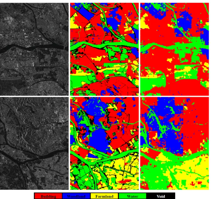
Fig. 5: TerraSAR-X image labeling results, the first column shows two regions (each 8800 × 6400 pixels), the second column illustrates the corresponding ground truth, the last column is our labeling results of KHAM.
TABLE I: Labeling accuracies of different labeling methods with different features(%)
Method
Feature
SVM PAM KAM PHAM KHAM GLCM 64.5 70.3 69.1 73.4 71.9
Gabor 65.8 71.1 69.5 74.9 73.5 GMRF 69.1 74.8 74.5 78.7 77.6 Hist 70.3 82.7 81.0 85.3 84.1
C. Discussions
This section analyzes and discusses some details of our labeling method.
1) Benefits of Aspect Model: The first main conclusion
from TABLE I is that our labeling methods are all significantly outperform SVM. With the same pixel-level training data, PAM exceeds SVM in labeling accuracy at least more than 5.3% no matter what features to use. Although used keywords-labeled training data, KAM also outperforms SVM by 3.7%. This is mainly due to our methods take the advantages of aspect models which can capture thematic coherence (image-wide correlations) and can resolve some cases of visual pol-ysemy. We may also benefit from bag-of-features (clustering) techniques which can discover image primitives and reduce noise effects at a certain degree.
2) Benefits of Incorporating Multi-scale Cues and Image Context: The second main conclusion from TABLE I is that HMAM is superior to aspect model at a single scale in image
Fig. 6: Subimages labeling results with KAM and KHAM, the first row shows four subimges (800 × 800 pixels), the second and the third rows illustrate their labeling results with KAM and KHAM, respectively, and the final row shows their ground truth.
labeling. With the help of multi-scale cues and image context, PHAM increases labeling results by 3% for PAM, and KHAM also increases labeling results by 3% for KAM. TABLE II and III indicate that multi-scale information and image context are more important for building area, while provide less help for farmland, woodland and water regions. It is maily because different patches in farmland basically have the same statistical properties, and the same case in woodland and water area. Therefore, there is little complementary information between neighboring patches in these scenes, and also the same case
between parent and children. However, patches in building area may different from each other significantly. Hence, some patches with high probabilities can disambiguate their neigh-bors, parent, or children. All in all, multi-scale cues and image context are more useful in dealing with complex scenes. Fig.6 illustrates four groups of subimage labelings of KAM and HKAM, from which we can see the incorporation of multi-scale cues and image context can really disambiguate some patches.
TABLE II: Labeling results of KAM(%)
Terrain Class Building Woodland Farmland Water Building 84.6 6.5 4.4 4.5 Woodland 20.0 63.7 13.1 3.0 Farmland 8.0 6.6 83.4 2.0 Water 7.5 1.4 3.0 88.2
TABLE III: Labeling results of KHAM(%)
Terrain Class Building Woodland Farmland Water Building 89.4 3.3 3.9 3.3 Woodland 20.8 64.8 12.1 2.3 Farmland 8.2 4.7 83.8 3.4 Water 6.2 1.3 3.3 89.3
3) Benefits of learning from keywords-labeled data: The
third main conclusion from TABLE I is that KAM and KHAM can achieve comparative performance to PAM and PHAM re-spectively, while the former only use keyword-labeled training data. It is a great merit for SAR imagery labeling, because it is expensive and labor-intensive to manually label each pixel in SAR images while it is convenient to obtain keywords-labeled training data. This property ensure the generalization of our methods to large-scale SAR imagery labeling.
4) Feature Comparison and Speed: Consequently, it is
important to select the features that are most informative for separating land-cover classes. From TABLE I, we learn that histogram is a simple but informative descriptor for SAR imagery labeling. Texture-based features such as GLCM, Gabor and GMRF achieve lower performance than histogram in our experiments. TABLE IV lists the computing speed of our methods and the benchmark methods. Currently, our un-optimized matlab implementation runs on a 2.4 GHz Pentium-class machine with 4G memory. TABLE IV also conclude that our methods are efficient both in training and test. Compared to PAM and KAM, PHAM and KHAM require more training and test time. The increased expenses are directly proportional to𝐿.
5) Labeling as function of the proportion of training data:
We now consider how the performances of our labeling methods drop as the proportion of training data decreases. We vary the proportion of training data versus the whole data (training+test) from 0.1 to 0.9. PAM, KAM, PHAM, and KHAM have the very similar tendency. Here, we only illustrate the experimental results of KHAM in Fig.7. We can conclude from Fig.7 that our labeling methods can achieve satisfactory
TABLE IV: Training and test speeds of different labeling methods
Method Training Time Test Time
ML - <0.01 sec/image
SVM 15 sec/image <0.01 sec/image
PAM - <0.1 sec/image
KAM < 0.1 sec/image <0.1 sec/image PHAM <0.05 sec/image 0.3 sec/image KHAM 0.3 sec/image 0.3 sec/image
0 0.2 0.4 0.6 0.8 1 0.8 0.81 0.82 0.83 0.84 0.85 0.86 0.87 Proportion (training/total) Labeling accurcy
Fig. 7: Labeling accuracy of KHAM when learning from increased proportion of training data.
performance even with small training dataset. V. CONCLUSION
In this study, we have addressed the challenge of labeling a whole scene of SAR imagery, and presented a solution by weakly supervised learning semantic classes from training samples that are labeled with image-level keywords rather than with detailed pixel-level detailed labeling. The proposed HMAM is shown to be promising for semantic labeling of SAR imagery, and it outperforms other used methods due to its complementary as aspect model use global relevance estimates while quadtree can further explore image context and multi-scale cues. We compared four different features and observed that using the simple histogram feature for the PLSA-image representation can achieve the highest performance in our experiments. Future work will focus on multiple features combination with multi-modal aspect model to further improve the labeling performance.
ACKNOWLEDGMENT
This work were supported in part by the National Natu-ral Science Foundation of China (No.40801183,60890074), the National High Technology Research and Development Program of China (No.2007AA12Z180,155)and CLASS (IST project 027978, funded by the European Union Information Society Technologies unit E5 C Cognition).
REFERENCES
[1] V. Venkatachalam, H. Choi, R.G. Baraniuk, “Multiscale SAR im-age segmentation using wavelet- domain hidden markov tree model,” in Proceedings of the SPIE lJth International Symposium on
Aerospace/Defense Sensing, Simulation, and Controls, Algorithms for Synthetic Aperture Radar Imagery VII, vol. 3497, pp. 110-120, 2000
[2] C. Tison, J. M. Nicolas, F. Tupin, and H. Maˆıre, “A New Statistical Model for Markovian Classification of Urban Areas in High-Resolution SAR Images,” IEEE Trans. Geosci. Remote Sens., vol. 42, no. 10, pp. 2046-2057, 2004.
[3] H.W. Deng, D.A. Clausi, “Unsupervised segmentation of synthetic aperture radar sea ice imagery using a novel Markov random field model,” IEEE Trans. Geosci. Remote Sens., vol. 43, no. 3, pp. 528-538, 2005.
[4] Y. Yang, H. Sun, and C. He, “Supervised SAR image MPM segmentation based on region-based hierarchical model,” IEEE Geosci. Remote Sens.
Lett., vol. 3, no. 4, pp. 517-521, 2006.
[5] G.-S. Xia, C. He, H. Sun, “Integration SAR Image Segmentation Method Using MRF on Region Adjacency Graph,” IET Radar, Sonar and
Navigation, Vol. 1, No. 5, pp. 348-354, 2007.
[6] G.-S. Xia, C. He, H. Sun, “A Rapid and Automatic MRF-based Clus-tering Method for SAR Images,”, IEEE Geosci. Remote Sens. Lett., Vol. 4, No. 4, pp. 596-600, 2007.
[7] Y.H.Wu, K.F. Ji, W.X. Yu and Yi Su, “Region-Based Classification of Polarimetric SAR Images Using Wishart MRF”, IEEE Geosci. Remote
Sens. Lett., Vol. 5, No. 4, pp. 668-672, 2008.
[8] J. A. Karvonen, “Baltic Sea Ice SAR Segmentation and Classification Using Modified Pulse-Coupled Neural Networks,”, IEEE Trans. Geosci.
Remote Sens., vol. 42, no. 7, pp.1566-1574, 2004
[9] M.Shimoni,D.Borghys,R.Heremans,C.Perneel, M.Acheroy. “Fusion of PolSAR and PolInSAR data for land cover classification,” Int.J.Applied
Earth Observation and Geoinformation, vol. 11, no. 3, pp. 169-180, Jun.
2009.
[10] X.L.She, J.Yang, W.J.Zhang. “The boosting algorithm with application to polarimetric SAR image classification,” in the First Asia-Pacific
Conference on Synthetic Aperture Radar (APSAR), pp. 779-783, Nov.
2007.
[11] J.Chen, Y.Chen, J.Yang. “A novel supervised classification scheme based on Adaboost for Polarimetric SAR Signal Processing,” in 9th
International Conference on Signal Processing, pp. 2400-2403, 2008.
[12] C. Lardeux, P.-L. Frison, C. Tison, J.-C. Souyris, B. Stoll, B. Fruneau, and J.-P. Rudant, “Support Vector Machine for Multifrequency SAR Polarimetric Data Classification,” IEEE Trans. Geosci. Remote Sens., to be appear, 2009.
[13] W.Yang, T.Y.Zou, D.X.Dai, Y.M.Shuai, “Supervised Land-cover Classi-fication of TerraSAR-X Imagery over Urban Areas Using Extremely Randomized Forest,” in 2009 Urban Remote Sensing Joint Event, shanghai, china, 20-22 May, 2009.
[14] T. Hofmann, “Unsupervised learning by probabilistic latent semantic anaylysis,” Machine Learning, vol. 42,no. 1-2, pp. 177-196, 2001. [15] D. Blei, A. Ng, and M. Jordan, “Latent Direchlet allocation,” Journal
of Machine Learning Research, vol. 3, no. 3, pp. 993-1022, 2003.
[16] M. Li´enou, H. Maˆıre, M. Datcu, “Semantic Annotation of Satellite Images Using Latent Dirichlet Allocation, ” IEEE Geosci. Remote Sens.
Lett., to be appeared, 2009.
[17] J. Verbeek, B. Triggs, “Region Classification with Markov Field As-pect Models,” in Proc. IEEE CS Conf. Computer Vision and Pattern
Recognition. 2007.
[18] L. Cao and L. Fei-Fei, “Spatially Coherent Latent Topic Model for Concurrent Segmentation and Classification of Objects and Scenes,” in
Proc. 11th Int’l Conf. Computer Vision, 2007.
[19] E. Xing, R. Yan, and A. Hauptmann, “ Mining associated text and images with dual-wing harmoniums,” in Proc. of the 21th Annual Conf. on
Uncertainty in Artificial Intelligence, AUAI press, 2005.
[20] W. Li , A. McCallum, “ Pachinko allocation: DAG-structured mixture models of topic correlations,” in Proc.23th Int’l Conf. Machine Learning, pp. 577-584, 2006.
[21] F.-F. Li and P. Perona. “A bayesian hierarchical model for learning natural scene categories,” in Proc. IEEE CS Conf. Computer Vision and
Pattern Recognition, pp. 524-531, 2005.
[22] A. Dempster, N. Laird, and D. Rubin, “Maximum likelihood from incomplete data via the EM algorithm,” Journal of the Royal Statistical
Sociaty, Series B, vol. 39, pp. 1-38, 1977.
[23] J.M. Laferte, P. Perez, and F. Heitz, “Discrete Markov image modeling and inference on the quadtree,” IEEE Trans. Image Process., vol. 9, no. 3, pp. 390-404, 2000.
[24] G.D. Forney, “The Viterbi algorithm,” in Proc. IEEE, vol. 61, no. 3, pp. 268-278, 1973.
[25] J. Yedidia, W. Freeman, and Y. Weiss, “Understanding belief propaga-tion and its generalizapropaga-tions,” Technical Report TR-2001-22, Mitsubishi Electric Research Laboratories, 2001.
[26] R.M. Haralick, K. Shanmugan, and I. Dinstein, “Textural features for image classification,” IEEE Trans. Syst. Man. Cybern, vol. 8, no. 6, pp. 610-621, 1973.
[27] A.K. Jain, and F. Farrokhnia, “Unsupervised texture segmentation using Gabor filters,” Pattern Recognition. vol. 24, no. 12, pp. 1167-1186, 1991.
[28] R. Chellappa, “Two-dimensional discrete Gaussian Markov random field models for image processing,” in Machine Intelligence and Pattern
Recognition: Progress in Pattern Recognition 2, G.T. Toussaint (Ed.),
Elsevier Science Publishers, B.V. (North-Holland). pp. 79-112, 1985. [29] D.A. Clausi, “Comparison and fusion of co-occurrence, Gabor, and MRF
texture features for classification of SAR sea ice imagery,” Atmosphere
& Oceans, vol. 39, no. 4, pp. 183-194, 2001.
[30] V. Kyrki, J. K. K¨am¨ar¨ainen, H. K¨alvi¨ainen, “Simple Gabor Feature Space for Invariant Object Recognition,” Pattern Recognit. Lett., vol. 25, no. 3 pp. 311-318, 2004.
[31] C. Corinna and V. Vapnik, “Support-Vector Networks,” Machine
Learn-ing, vol. 20, pp. 273-291, 1995.
[32] C.C. Chang and C.J. Lin, “LIBSVM : a library for support vector machines,” 2001. Software available at:
http://www.csie.ntu.edu.tw/∼cjlin/libsvm
Wen Yangreceived his Ph.D. from Wuhan Univer-sity, China, in 2004. He is currently an associate professor at the School of Electronic Information, Wuhan University. His research interests include im-age segmentation and classification, target detection and recognition, machine learning and data mining with applications to remote sensing.
Dengxin Dai received B.S. degree in optical in-formation science and technology in 2008, from Wuhan University, Wuhan, Hubei, China, where he is currently working toward the Ph.D degree at the signal processing laboratory, school of electronic information. His research interests include image processing, computer vision, and machine learning.
Bill Triggs originally trained as a mathematical physicist at Auckland, Australian National, and Ox-ford Universities. He has worked extensively on vision geometry (matching constraints, scene re-construction, autocalibration) and robotics, but his current research focuses on computer vision, pattern recognition, and machine learning for visual object recognition and human motion understanding. Now he works in (and is deputy director of) the Labora-toire Jean Kuntzmann (LJK) in Grenoble in the heart of the French Alps.
Gui-Song Xia received the B.S and M.S. degree in Electronic Engineering from Wuhan University, Wuhan, China, in 2005 and 2007, respectively.He is currently pursuing his Ph.D degree at French National Center for Scientific Research (CNRS) -Information Processing and Communication Labora-tory (LTCI), Institute Telecom, Telecom ParisTech, Paris, France. His research interests include image analysis, computer vision, learning in vision, image processing and remote sensing.