Titre:
Title:
Measuring and visualizing space–time congestion patterns in an urban road network using large-scale smartphone-collected GPS data
Auteurs:
Authors:
Joshua Stipancic, Luis Miranda-Moreno, Aurélie Labbe et Nicolas Saunier
Date: 2019
Type: Article de revue / Journal article
Référence:
Citation:
Stipancic, J., Miranda-Moreno, L., Labbe, A. & Saunier, N. (2019). Measuring and visualizing space–time congestion patterns in an urban road network using large-scale smartphone-collected GPS data. Transportation Letters, p. 1-11.
doi:10.1080/19427867.2017.1374022 Document en libre accès dans PolyPublie
Open Access document in PolyPublie
URL de PolyPublie:
PolyPublie URL: https://publications.polymtl.ca/2973/
Version: Version finale avant publication / Accepted version Révisé par les pairs / Refereed Conditions d’utilisation:
Terms of Use: Tous droits réservés / All rights reserved
Document publié chez l’éditeur officiel
Document issued by the official publisher
Titre de la revue:
Journal Title: Transportation Letters
Maison d’édition:
Publisher: Taylor and Francis
URL officiel:
Official URL: https://doi.org/10.1080/19427867.2017.1374022
Mention légale:
Legal notice:
This is an Accepted Manuscript of an article published by Taylor & Francis in
Transportation Letters on 2019, available online:
http://www.tandfonline.com/10.1080/19427867.2017.1374022. Ce fichier a été téléchargé à partir de PolyPublie, le dépôt institutionnel de Polytechnique Montréal
This file has been downloaded from PolyPublie, the institutional repository of Polytechnique Montréal
Measuring and Visualizing Space-Time Congestion Patterns in an Urban
Road Network Using Large-Scale Smartphone-Collected GPS Data
Joshua Stipancic
a*, L. Miranda-Moreno
a, A. Labbe
b, and N. Saunier
ca Department of Civil Engineering and Applied Mechanics, McGill University, Montreal,
Quebec, Canada; b Department of Decision Sciences, HEC Montréal, Montreal, Quebec,
Canada; c Department of Civil, Geological and Mining Engineering, Polytechnique
Montréal, Montreal, Quebec, Canada
* Room 391, Macdonald Engineering Building, 817 Sherbrooke Street West, Montréal, Québec, Canada H3A 0C3, [email protected]
2
Measuring and Visualizing Space-Time Congestion Patterns in an Urban
Road Network Using Large-Scale Smartphone-Collected GPS Data
Congestion is a dynamic phenomenon with elements of space and time, making it a promising application of probe vehicles. The purpose of this paper is to measure and visualize the magnitude and variability of congestion on the network scale using smartphone GPS travel data. The sample of data collected in Quebec City contained over 4000 drivers and 21,000 trips. The congestion index (CI) was calculated at the link level for each hour of the peak period and congestion was visualized at aggregate and disaggregate levels. Results showed that each peak period can be viewed as having an onset period and dissipation period lasting one hour. Congestion in the evening is greater and more dispersed than in the morning. Motorways, arterials, and collectors contribute most to peak period congestion, while residential links contribute little. Further analysis of the CI data is required for practical implementation in network planning or congestion remediation.
Keywords: congestion; visualization; smartphone; GPS; space-time patterns Subject classification codes: 2.4; 9.1; 9.2; 9.8; 9.9; 9.10
Introduction
For transportation professionals, accurate and quantitative performance measures are needed to operate existing networks and plan future facilities (D'Este, Zito and Tayler 1999). For drivers, network performance influences travel choices (Liu and Ma 2009). Link or route travel time is a common performance measure of importance for road users and practitioners alike (Li and McDonald 2002). Although travel time is a key parameter defining traffic state (Zhang 1999) and is easily understood by the public (Liu and Ma 2009), it may not be the biggest factor influencing travel decisions. Traffic congestion occurs on a roadway ‘when demand … exceeds its ability to supply an acceptable level of service’ (D'Este, Zito and Tayler 1999), and can greatly affect travel time reliability. Road users are willing to accept longer travel times if they can be assured that they will usually arrive on time (Taylor 2013).
3
In other words, users may choose a route with a longer travel time in order to avoid congestion and decrease potential travel time variability (D'Este, Zito and Tayler 1999). Traffic congestion is worsening in many urban areas (Taylor, Woolley and Zi 2000), where traditional expectations of peak period congestion are being replaced by congestion lasting throughout the day. Efforts to understand and reduce the ‘extent, duration, and intensity’ of congestion (Sioui and Morency 2013) should be a high priority (Taylor, Woolley and Zi 2000).
Detailed road network congestion information would be beneficial for both
transportation professionals and the public. Recently, new traffic sensors, including radar, magnetic, and video-based devices, have been developed, and advances in management practices have ‘increased [the] need for very accurate road traffic information’ (El Faouzi, Leung and Kurian 2011). Congestion ‘is a dynamic phenomenon with elements of both space and time’ (D'Este, Zito and Tayler 1999) and requires temporal and spatial data coverage, making it a promising application of probe vehicles, one of the only methods currently capable of providing such data. Probe vehicles act ‘as moving sensors, continuously feeding information about traffic conditions’ (El Faouzi, Leung and Kurian 2011) through continuous instrumentation and tracking, allowing for a precise measurement of route or link travel time for vehicles operating within normal traffic (Li and McDonald 2002). Although several methods for instrumenting vehicles exist, GPS data has been shown to be reliable in several applications (Jun, Ogle and Guensler 2007). While traditional floating car studies have been limited in driver sample size and spatio-temporal coverage (Liu and Ma 2009), GPS-enabled smartphones have the potential to increase the number of drivers sampled, increase temporal coverage to several weeks or months, and increase the spatial coverage to include the entire road network.
4
Although GPS probe vehicles have been successfully implemented in freeways (Quiroga and Bullock 1998), specific consideration for urban environments is required. Tall buildings in urban centers can completely block GPS signals or create spurious signals (D'Este, Zito and Tayler 1999), leading to positional noise which must be corrected. Sufficient network coverage is practically limited by driver sample size, regardless of the collection method. Additionally, methods for automating data handling and analysis are required due to large data volumes obtained through smartphone data collection. Other challenges include selecting appropriate measures of congestion to represent magnitude and variability across time and space. Despite technological advancement and increasing
congestion levels, smartphone-based systems for measuring and monitoring traffic congestion are still rare in North American cities (Chen and Chien 2000), and ‘literature in network level dynamics and congestion propagation is limited especially in large urban networks’
(Saeedmanesh and Geroliminis 2016). The purpose of this paper is to present a methodology for measuring and visualizing the magnitude and variability of congestion on the network scale using smartphone GPS data collected from regular drivers. The three primary objectives are:
(1) To process network-wide GPS travel data;
(2) To quantify congestion on the network scale using the Congestion Index (CI); and, (3) To visualize changes in congestion levels across time and space at aggregate and
disaggregate scales.
Literature Review
Existing methods for estimating road traffic conditions depend predominantly on the source of traffic data. Using fixed point traffic sensors, the naïve method uses spot speeds that, when combined with flow, density, and speed relationships, can define traffic conditions (Dailey
5
1993). This method may introduce a systematic bias (Ostrand, et al. 1997) as detector data ‘only reflect conditions averaged over a fixed time period at a single point in space’ whereas traffic flow ‘reflects traffic conditions averaged over a fixed distance and a variable amount of time’ (Coifman 2002). In trajectory methods, trajectories of simulated vehicles are
constructed based on traffic data observed by several consecutive fixed sensors (van Lint and van der Zijpp 2007). van Lint and van der Zijpp (2007) improved traditional methods by assuming linear speed variation (rather than piecewise-constant variation), which more accurately represents spatially and temporally dependent flow variation. Coifman (2002) constructed trajectories based on several loop detectors to estimate travel time in a freeway environment, demonstrating that estimated travel times were within 10 % of actual travel times on average. Liu and Ma (2009) fused loop data with signal phase information in urban corridors to estimate travel times generally within 5 % of ground truth. As with the naïve method, trajectory methods are limited because data is collected at discrete locations (Coifman 2002).
Vehicle reidentification (VRI) is ‘the process of matching vehicles from one point on the roadway … to the next’ (Sun, et al. 2004) based on a reproducible feature or vehicle signature (Coifman and Krishnamurthy 2007). When a vehicle is identified at two locations within the network, the travel time between those locations is determined. Vehicle signatures may be captured using license plate recognition (Anagnostopoulos, et al. 2006) or media access control addresses captured from Bluetooth devices within passing vehicles (Haseman, Wasson and Bullock 2010), though most Bluetooth detectors have a detection rate of 5 % or less (Haghani, et al. 2010). Vehicle length (Coifman and Cassidy 2002) and magnetic signature (Kwong, et al. 2009) have also been used to define vehicle signature. Coifman and Cassidy (2002) reidentified 20 % of vehicles based on length, and Sun et al. (2004) used inductive loops and feature-based colour extracted from video stills to achieve an
6
approximately 90 % match rate. Kwong et al. (2009) used permanent wireless magnetic sensors installed across several intersections along an urban corridor. The authors estimate a successful matching rate of 65-75 % (Kwong, et al. 2009). Besides less than ideal detection rates, a limitation of VRI is that the accuracy depends on the distance between sensors. As distance between sensors increases, so do the unknowns of the vehicle’s path, decreasing the likelihood that the sensors actually measure travel time along the shortest path.
Traditionally, floating cars have been popular for estimating traffic volumes, speeds, and travel times. Techniques for estimating travel time vary depending on the number of vehicles utilized. One approach uses the average travel time from a relatively large number of floating cars operating within the same time and space. However, the labor requirement associated with floating cars is high (Chen and Chien 2000), and approaches have been developed to use relatively fewer vehicles with statistical adjustments to extrapolate floating car travel time to mean travel time (Yang 2005). For example, Li and McDonald (2002) proposed an approach using only a single vehicle, using the driving pattern of the floating car to estimate the difference between the vehicle and average traffic conditions. Probe vehicles, with continuous spatio-temporal tracking, have become a popular method for measuring traffic conditions (Quiroga and Bullock 1998), and represent substantial improvement over methods using fixed sensors or floating cars. Initial work by D’Este, Zito, and Taylor (1999) explored the feasibility of using GPS to collect traffic data, concluding that GPS was ‘a relatively cheap, efficient and effective means’. GPS data collected from the smartphones of regular drivers enables the use of a large number of probe vehicles without the high labor costs associated with traditional floating cars. Additionally, data from regular drivers may better represent typical traffic conditions (Stipancic, Miranda-Moreno and Saunier 2016).
Measures of congestion are typically based on either travel time or speed (Shi and Abdel-Aty 2015). Congestion may be measured as a change in travel time (Palen 1997) from
7
a baseline or expected travel time measurement (Coifman 2002). Measures like travel time index (TTI) use the ratio of travel time to off-peak travel time to determine congestion at the link level (Falcocchio and Levinson 2015). TTI and similar techniques can be used to derive historical trend data to separate recurring and non-recurring congestion (Coifman 2002). Skabardonis, Varaiya, and Petty (2003) utilized a delay-based approach to separate recurrent from non-recurrent delay. In Washington State, mean speeds below 75 % of free flow speed are used to define the onset of congestion (Falcocchio and Levinson 2015). In Quebec, a threshold of 60 % is used (ADEC 2014). The Congestion Index (CI) was proposed by Dias et al. (2009) as the difference between the actual speed and free flow speed over the free flow speed. Although CI and other indices are limited to calculations on a particular link or route, they ‘can be used for an urban area wide application’ (Aftabuzzaman 2007). With GPS probe vehicles, congestion measures based on spot speed measurements are preferred. Travel time estimation may be influenced by errors in the reported GPS coordinates and on assumptions of the start and end of trip (or link). Considering the relatively recent advent of GPS data in transportation research, several shortcomings remain in the literature. Few studies have considered the rich source of data available from GPS-enabled smartphones. Congestion studies using probe vehicles have primarily focused on the corridor-level without
consideration for estimating travel time or congestion at the network level. Despite successful probe vehicle studies in freeways, additional focus on urban roadways is required.
Methodology
Data Structure
GPS data from the smartphones of regular drivers contains observations describing the entirety of their trip, both across time and across the road network. For each trip, 𝑖𝑖, logged into a smartphone application, GPS travel data is returned as a series of observations, 𝑂𝑂𝑖𝑖𝑖𝑖,
8 such as 𝑡𝑡𝑡𝑡𝑖𝑖𝑡𝑡𝑖𝑖 = ⎩ ⎪ ⎨ ⎪ ⎧𝑂𝑂𝑂𝑂𝑖𝑖0𝑖𝑖1 ⋮ 𝑂𝑂𝑖𝑖𝑖𝑖 ⋮ 𝑂𝑂𝑖𝑖𝑖𝑖𝑖𝑖⎭ ⎪ ⎬ ⎪ ⎫ = ⎩ ⎪ ⎨ ⎪ ⎧ 𝑖𝑖, 𝑐𝑐𝑖𝑖, 𝑐𝑐𝑖𝑖0𝑖𝑖1, 𝑡𝑡, 𝑡𝑡𝑖𝑖0𝑖𝑖1, 𝑥𝑥, 𝑥𝑥𝑖𝑖1𝑖𝑖0, 𝑦𝑦, 𝑦𝑦𝑖𝑖1𝑖𝑖0, 𝑧𝑧, 𝑧𝑧𝑖𝑖1𝑖𝑖0, 𝑣𝑣, 𝑣𝑣𝑖𝑖0𝑖𝑖1 ⋮ 𝑖𝑖, 𝑐𝑐𝑖𝑖𝑖𝑖, 𝑡𝑡𝑖𝑖𝑖𝑖, 𝑥𝑥𝑖𝑖𝑖𝑖, 𝑦𝑦𝑖𝑖𝑖𝑖, 𝑧𝑧𝑖𝑖𝑖𝑖, 𝑣𝑣𝑖𝑖𝑖𝑖 ⋮ 𝑖𝑖, 𝑐𝑐𝑖𝑖𝑖𝑖𝑖𝑖, 𝑡𝑡𝑖𝑖𝑖𝑖𝑖𝑖, 𝑥𝑥𝑖𝑖𝑖𝑖𝑖𝑖, 𝑦𝑦𝑖𝑖𝑖𝑖𝑖𝑖, 𝑧𝑧𝑖𝑖𝑖𝑖𝑖𝑖, 𝑣𝑣𝑖𝑖𝑖𝑖𝑖𝑖⎭ ⎪ ⎬ ⎪ ⎫
where 𝑖𝑖 is a unique trip identifier, 𝑂𝑂𝑖𝑖𝑖𝑖 is the jth observation in trip 𝑖𝑖, 𝑐𝑐𝑖𝑖𝑖𝑖 is a unique coordinate identifier, 𝑡𝑡𝑖𝑖𝑖𝑖 is the datetime, 𝑥𝑥𝑖𝑖𝑖𝑖, 𝑦𝑦𝑖𝑖𝑖𝑖, and 𝑧𝑧𝑖𝑖𝑖𝑖 are the latitude, longitude, and altitude, and 𝑣𝑣𝑖𝑖𝑖𝑖 is the speed. From each trip, several key pieces of trip information include the origin (𝑥𝑥𝑖𝑖0, 𝑦𝑦𝑖𝑖0) and destination (𝑥𝑥𝑖𝑖𝑖𝑖𝑖𝑖, 𝑦𝑦𝑖𝑖𝑖𝑖𝑖𝑖) and start (𝑡𝑡𝑖𝑖0) and end times (𝑡𝑡𝑖𝑖𝑖𝑖𝑖𝑖). Total travel time can also be
computed (𝑡𝑡𝑖𝑖𝑖𝑖𝑖𝑖− 𝑡𝑡𝑖𝑖0). The time between consecutive observations is typically between 1 and
2 seconds. Depending on the application, socio-demographic information may also be
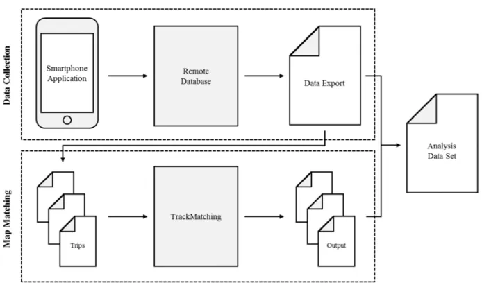
available. Once a trip has been collected and reported by the user, initial pre-processing of the data using methods including Kalman filtering (Bachman 2011) to reduce variability are typical. The data is then stored in a database from which observations are exported for analysis.
Map Matching
Although the raw GPS data from a smartphone application are spatio-temporally rich, position is provided only in terms of latitude and longitude and is not linked spatially to the road network. If the goal is to determine congestion at the link level, then it is necessary to explicitly match each trip to the travelled network links. A map matching procedure ensures that traffic conditions extracted from the trip data are correctly assigned to the links in which the traffic conditions are occurring. TrackMatching is a commercially available, cloud-based web map-matching software service (F. Marchal 2015) that matches GPS trip data to the OpenStreetMap (OSM) road network (OpenStreetMap 2015). Before GPS data is sent to
9
TrackMatching, the data is split into individual trips and formatted according to the software input requirements, including only the coordinate ID, timestamp, latitude, and longitude for each observation. The software returns a new latitude and longitude, 𝑥𝑥𝑖𝑖𝑖𝑖′ and 𝑦𝑦𝑖𝑖𝑖𝑖′, which correspond to a specific OSM link ID, 𝑙𝑙𝑖𝑖𝑖𝑖, as shown below.
�𝑐𝑐𝑖𝑖𝑖𝑖, 𝑡𝑡𝑖𝑖𝑖𝑖, 𝑥𝑥𝑖𝑖𝑖𝑖, 𝑦𝑦𝑖𝑖𝑖𝑖� → TrackMatching → �𝑐𝑐𝑖𝑖𝑖𝑖, 𝑡𝑡𝑖𝑖𝑖𝑖, 𝑥𝑥𝑖𝑖𝑖𝑖′ , 𝑦𝑦𝑖𝑖𝑖𝑖′, 𝑙𝑙𝑖𝑖𝑖𝑖, 𝑠𝑠𝑖𝑖𝑖𝑖, 𝑑𝑑𝑖𝑖𝑖𝑖�
𝑥𝑥𝑖𝑖𝑖𝑖′ and 𝑦𝑦𝑖𝑖𝑖𝑖′ are chosen based on the Euclidean distance from the raw GPS points to the nearest link and on network topology (Marchal, Hackney and Axhausen 2005). Track Matching also returns the source, 𝑠𝑠𝑖𝑖𝑖𝑖, and destination nodes, 𝑑𝑑𝑖𝑖𝑖𝑖, which can be used to identify direction of travel along the link. The algorithm generates a set of candidate paths and assigns the trip to the most probable path from origin to destination. After map-matching is completed, each observation corresponds to an exact location within the road network, and the series of links can be used to define the route from origin to destination. Once merged with the original data, the complete data set is as shown below.
𝑡𝑡𝑡𝑡𝑖𝑖𝑡𝑡𝑖𝑖 = ⎩ ⎪ ⎪ ⎨ ⎪ ⎪ ⎧ 𝑖𝑖, 𝑐𝑐𝑖𝑖, 𝑐𝑐𝑖𝑖0, 𝑡𝑡𝑖𝑖0, 𝑥𝑥𝑖𝑖1′ , 𝑦𝑦𝑖𝑖0′ , 𝑧𝑧𝑖𝑖0, 𝑣𝑣𝑖𝑖0, 𝑙𝑙𝑖𝑖0, 𝑠𝑠𝑖𝑖0, 𝑑𝑑𝑖𝑖0 𝑖𝑖1, 𝑡𝑡𝑖𝑖1, 𝑥𝑥𝑖𝑖1′ , 𝑦𝑦𝑖𝑖1′ , 𝑧𝑧𝑖𝑖1, 𝑣𝑣𝑖𝑖1, 𝑙𝑙𝑖𝑖1, 𝑠𝑠𝑖𝑖1, 𝑑𝑑𝑖𝑖1 ⋮ 𝑖𝑖, 𝑐𝑐𝑖𝑖𝑖𝑖, 𝑡𝑡𝑖𝑖𝑖𝑖, 𝑥𝑥𝑖𝑖𝑖𝑖′ , 𝑦𝑦𝑖𝑖𝑖𝑖′, 𝑧𝑧𝑖𝑖𝑖𝑖, 𝑣𝑣𝑖𝑖𝑖𝑖, 𝑙𝑙𝑖𝑖𝑖𝑖, 𝑠𝑠𝑖𝑖𝑖𝑖, 𝑑𝑑𝑖𝑖𝑖𝑖 ⋮ 𝑖𝑖, 𝑐𝑐𝑖𝑖𝑖𝑖𝑖𝑖, 𝑡𝑡𝑖𝑖𝑖𝑖𝑖𝑖, 𝑥𝑥𝑖𝑖𝑖𝑖′ 𝑖𝑖, 𝑦𝑦𝑖𝑖𝑖𝑖′ 𝑖𝑖, 𝑧𝑧𝑖𝑖𝑖𝑖𝑖𝑖, 𝑣𝑣𝑖𝑖𝑖𝑖𝑖𝑖, 𝑙𝑙𝑖𝑖𝑖𝑖𝑖𝑖, 𝑠𝑠𝑖𝑖𝑖𝑖𝑖𝑖, 𝑑𝑑𝑖𝑖𝑖𝑖𝑖𝑖⎭ ⎪ ⎪ ⎬ ⎪ ⎪ ⎫
The processes of data collection and map matching are illustrated in Figure 1. Network Definition
Although the map-matching procedure links each observation to the road network, the use of the OSM network in the TrackMatching algorithm presents a challenge. The majority of the network consists of five distinct functional classes: freeway, primary, secondary, tertiary, and
10
residential (where primary, secondary, and tertiary are arterials and collectors classified by importance to the road network, with primary being most important). Ideally, these links would never be divided by an intersection (Sioui and Morency 2013) (each link should connect adjacent intersections). The OSM road network is generated non-systematically by users, and OSM links do not always meet this definition. In urban centers, intersection design and operation can significantly impact congestion levels on consecutive links. It is desired to redefine the network such that each link is properly defined between adjacent intersections. Redefining the network requires several steps, which can be completed in any GIS software environment. The process is as follows:
(1) Identify all nodes that represent an intersection in the road network. In doing so, nodes that only define network topology, such as those used to define curves, are ignored.
(2) Split the road network at the identified nodes. Any links connecting more than two intersections are broken into several smaller links. Links already properly defined are unchanged.
(3) Rename each link according to its original ID and the nodes on either end of the link. Step 2 leaves several links with the same ID. In order for each link to have a unique identifier, the nodes on either end of the link are used to provide a unique ID.
(4) Remap the GPS observations to the new network. Travelled links in the GPS trip data are renamed using the same scheme as the mapping data, by concatenating the link ID, source node, and destination node into a unique identifier.
11 Computing Congestion Index
The map matching procedure enables congestion measurement for every link containing sufficient GPS data, providing either a disaggregate view of link performance, or an aggregate view of network performance. Aftabuzzaman (2007) suggested that congestion measures meet several criteria including clarity, simplicity, comparability, and continuity. As discussed, time-based measures have been proposed. However, because link travel time is dependent on position, and because the precise latitude and longitude are untrustworthy (and are in fact removed as part of the map matching procedure), a congestion measure based on speed measurements is preferred, even if those speeds are originally derived from the GPS positions. Dias et al. (2009) proposed the Congestion Index (CI) as one speed-based congestion measure, calculated as
𝐶𝐶𝐶𝐶 =free flow speed − actual speedfree flow speed if 𝐶𝐶𝐶𝐶 > 0 = 0 if 𝐶𝐶𝐶𝐶 ≤ 0
(1)
This formulation yields CI values ranging from 0 (speed equal to the free flow speed) and 1 (speed is zero), and meets several of the suggested criteria. The first necessary step is calculating the free flow speed on each link, 𝐿𝐿𝑖𝑖𝑖𝑖. Free flow speed has been defined in numerous ways, though as congestion is generally constrained to the AM and PM peak periods, the speeds observed outside of these times can be used to estimate free flow speed. For this project, the morning peak period was defined as 6:00 to 10:00 AM, and the evening peak from 3:00 to 7:00 PM. The off-peak time, 𝑇𝑇𝑜𝑜𝑜𝑜𝑜𝑜, includes all other times. Free flow speed on a given link, 𝐿𝐿𝑖𝑖𝑖𝑖, is calculated as the average of all observed speeds on 𝐿𝐿𝑖𝑖𝑖𝑖 during 𝑇𝑇𝑜𝑜𝑜𝑜𝑜𝑜, or
12 𝐹𝐹𝐹𝐹𝐹𝐹𝐿𝐿𝑖𝑖𝑖𝑖 =
∑ ∑ 𝑣𝑣𝑖𝑖 𝑖𝑖 𝑖𝑖𝑖𝑖
𝑁𝑁 (2)
where 𝑣𝑣𝑖𝑖𝑖𝑖 is the speed for every observation on link 𝐿𝐿𝑖𝑖𝑖𝑖 during 𝑇𝑇𝑜𝑜𝑜𝑜𝑜𝑜, and 𝑁𝑁 is the number of those observations. Next, the congestion index for every observation can be computed according to 𝐶𝐶𝐶𝐶𝑖𝑖𝑖𝑖 = 𝐹𝐹𝐹𝐹𝐹𝐹𝐿𝐿𝑖𝑖𝑖𝑖− 𝑣𝑣𝑖𝑖𝑖𝑖 𝐹𝐹𝐹𝐹𝐹𝐹𝐿𝐿𝑖𝑖𝑖𝑖 if 𝐹𝐹𝐹𝐹𝐹𝐹𝐿𝐿𝑖𝑖𝑖𝑖 > 𝑣𝑣𝑖𝑖𝑖𝑖 = 0 otherwise (3)
where 𝐶𝐶𝐶𝐶𝑖𝑖𝑖𝑖 is the congestion index for observation 𝑂𝑂𝑖𝑖𝑖𝑖, 𝐹𝐹𝐹𝐹𝐹𝐹𝐿𝐿𝑖𝑖𝑖𝑖 is the free flow speed on link
𝐿𝐿𝑖𝑖𝑖𝑖, and 𝑣𝑣𝑖𝑖𝑖𝑖 is the observed speed. As congestion levels vary across both distance and time, it is not only necessary to calculate CI at the link level, but also to calculate CI at different time intervals. The peak periods were divided into 60-minute time periods (one per hour) resulting in 8 total time periods. Therefore, the congestion index for link 𝐿𝐿𝑖𝑖𝑖𝑖 during time period 𝑇𝑇 is calculated as:
𝐶𝐶𝐶𝐶𝐿𝐿𝑖𝑖𝑖𝑖𝑇𝑇 =
∑ ∑ 𝐶𝐶𝐶𝐶𝑖𝑖 𝑖𝑖 𝑖𝑖𝑖𝑖
𝑁𝑁 (4)
where 𝐶𝐶𝐶𝐶𝑖𝑖𝑖𝑖 is the congestion index for observation 𝑂𝑂𝑖𝑖𝑖𝑖 on link 𝐿𝐿𝑖𝑖𝑖𝑖 during a time period 𝑇𝑇, and 𝑁𝑁 is the number of observations on link 𝐿𝐿𝑖𝑖𝑖𝑖 during 𝑇𝑇. To minimize noise, filters were added by setting minimum acceptable numbers of trips and observations for CI calculation. For a valid 𝐶𝐶𝐶𝐶𝐿𝐿𝑖𝑖𝑖𝑖𝑇𝑇, 𝐿𝐿𝑖𝑖𝑖𝑖 must contain at least 2 trips during time 𝑇𝑇, and each of those trips must have
at least 2 observations falling on link 𝐿𝐿𝑖𝑖𝑖𝑖. CI is calculated for bi-directional traffic using the source and destination nodes within the map matched data to define two unique links.
13 Data Visualization
After the data is processed and CI is calculated, congestion can be visualized throughout the network, as has been discussed by several authors (Kartika 2015). Although CI can be computed for any single hour on any given day, a single instant in time does not provide general insight which would be beneficial to transportation professionals or to the driving public. Congestion levels vary significantly throughout the day (due to variation in demand) and vary significantly between days (due to variation in demand and non-recurrent
phenomena including construction or crashes) and quantifying and/or visualizing this
variation using only GPS travel data would be a significant contribution to existing research. Firstly, congestion can be visualized using a disaggregate approach, where each link is considered individually. First, CI was calculated for each hour of the peak periods, by pooling together all of the weekday travel data in order to demonstrate hourly congestion variation on a typical weekday. Maps and animations were generated by coloring each link according to the congestion level observed during each hour. For this purpose, CI was divided into three categories; high congestion, CI of 0.30 or greater (consistent with
Washington State and Quebec guidelines); moderate congestion, CI of 0.15 to 0.30, and low congestion, CI of 0.00 to 0.15. A detailed understanding of congestion should include both the average level of congestion for a given link and some indication of how variable that level of congestion is from day to day. In order to capture variation between days, CI was also calculated for every hour of each weekday independently. The number of hours that each link experienced CI above 0.30 were summed, out of a possible 120 hours (8 peak hours per day over 15 weekdays). Maps were generated to show not only which links were most congested, but also to show which links were congested most consistently over the 15 days of study.
Although one strength of this type of analysis is that each link can be viewed independently, it may be difficult or impossible to make meaningful conclusions about the
14
behavior of the network in general. To facilitate observation of network-wide trends, it may be appropriate to aggregate the data in some way. Congestion does not occur all at once. Instead, it gradually builds and then subsides throughout the peak periods. Similarly,
congestion does not occur across all network links simultaneously. This study aggregated in two different ways; first by distance to the city center, and second by roadway functional classification. Aggregation by distance has the potential to show how congestion propagates with respect to the downtown core. To accomplish this, the city center was defined as the location of Quebec City Hall. Bins of 200 m distances were defined with respect to City Hall. The average CI was then computed for each distance bin for each hour of the day, by pooling together all of the weekday travel data. Next, links were categorized according to their OSM functional classification. The analysis was completed separately considering five distinct functional road classes: freeway, primary, secondary, tertiary, and residential. Using the pooled weekday data, the proportion of links experiencing high, moderate, and low congestion levels were computed and plotted for each hour for each of the five functional classes.
Results
Data Description
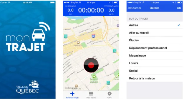
GPS travel data was collected in Quebec City, Canada using the Mon Trajet application (City of Quebec 2015) developed by BriskSynergies (2015). Screenshots from the application are shown in Figure 3. The application, which was available for Apple and Android devices, was installed voluntarily by drivers and allowed them to anonymously log trips into the
application. As part of the system developed by BriskSynergies, data is automatically uploaded and stored in a cloud-based platform. In total, approximately 5000 driver
15
is a sample of open data made available by the City of Quebec. The sample for this study contained over 4000 drivers and 21,939 individual trips during the period between April 28 and May 18, 2014. Over the 21 days sampled, 19.7 million individual data points were logged.
Disaggregate Visualization
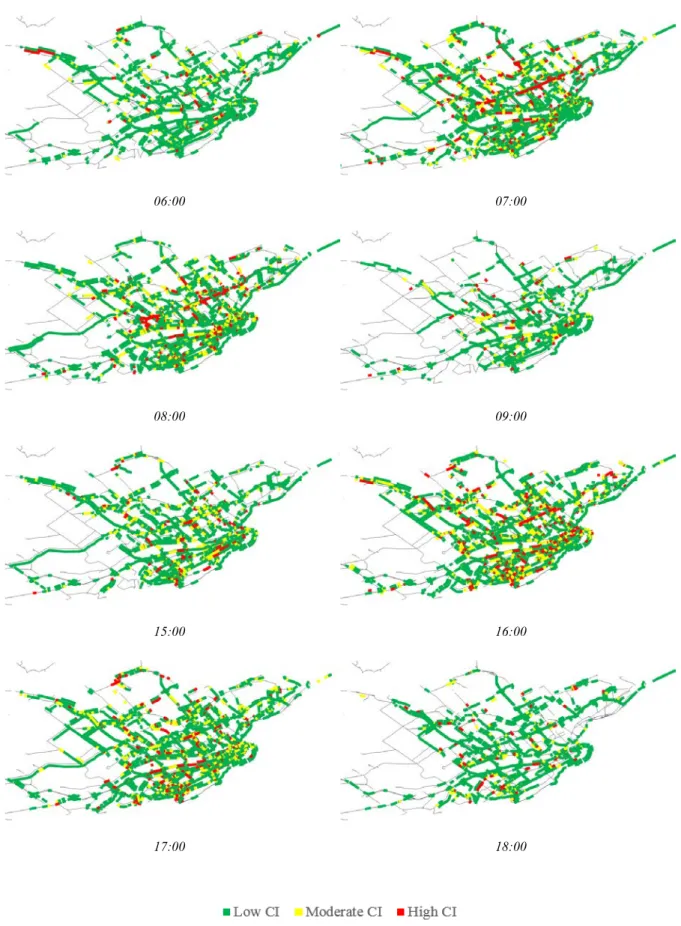
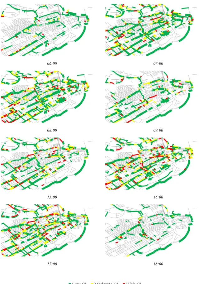
Figure 4 and Figure 5 present the level of congestion experienced throughout the road network for each of the eight AM and PM peak period hours, for the entire network and downtown respectively. As CI for these maps is based on pooled weekday data, the figures demonstrate the level of congestion expected on a typical weekday. In this pooled data set, containing fifteen weekdays of data, each peak hour contains CI measurements for between 6600 and 12,000 links. Considering the Quebec City network contains over 50,000 total links, this represents between 13 % and 24 % of the total road network. Although the collection campaign in Quebec City was large (the sample for this study contained nearly 22,000 trips), many network links, primarily residential streets, contain no observations. Still, the most critical links, including major freeways, arterials, and collectors, are well populated, and provide a good view of congestion trends across the network. In fact, those links that are missing data tend to be low volume streets were congestion is highly unlikely anyway. As with the total number of trips in the population, the total number of GPS trips logged varies with time, first growing to a maximum and then subsiding throughout the peak periods. This phenomenon is clearly observed in Figure 4 and Figure 5. For example, the period beginning at 6:00 PM has far fewer observations than the period beginning at 4:00 PM.
The results from these figures largely corroborate intuition. Take, for example, the AM peak period. Beginning at 6:00 AM, very few links are highly or moderately congestion (most links have CI < 0.15, so are operating at or near free flow speed). However, by 7:00
16
AM, the freeways and major arterials toward downtown become highly congested (CI
exceeds 0.30, and in some cases is as high as 0.85). A similar pattern is observed at 8:00 AM. However, by 9:00 AM, congestion has largely subsided on the freeways and arterials, while some streets in the downtown core remain congested. A mirror image of this pattern is observed in the PM peak period, with congestion beginning to form at 3:00 PM, highly congestion conditions at 4:00 PM and 5:00 PM, and dissipation at 6:00 PM. In this way, each 4-hour peak period can be roughly viewed as having an onset period (lasting approximately one hour), the peak itself (lasting approximately two hours), and a dissipation period (lasting approximately one hour).
Rather than pooling all weekday data together, each peak hour of every weekday can be considered separately. Each individual weekday yields at least one CI measurement for between 2000 and 4000 links (about 6 % of the network on an average day). For each individual peak period hour, there are between 250 and 1750 links with a CI measurement (between 0.5% and 3.5% of the total road network). Figure 6 shows the total number of hours that each link spent in the highly congested state (CI > 0.30). It was observed that the
majority of highly congested links are only highly congested for about 30 hours over the 15 study days (about 2 hours per day). However, for some links, the number of hours in the highly congested state are as high as 61. To provide some perspective, highly directional links, such as motorways and arterials which carry commuters towards the city center, experience peak flow for one peak period (either AM or PM). This relates to a possible 60 hours out of the total 120 peak period hours. Any link with nearly 60 hours in the highly congested state could be considered to be chronically congested (it is always highly
congested during either the AM or PM peak). The most consistently congested locations are Autoroute Felix-Leclerc, which runs east/west north of the city center, the interchange
17
connecting Autoroute Felix-Leclerc with Autoroute Henry-IV, and several arterial links near Laval University west of the city center.
Aggregate Visualizations
In order to observe some general trends in the formation and propagation of congestion within Quebec City, links were aggregated first according to distance to the city center, and second by functional classification. Figure 7 shows the average CI for each peak hour (calculated from the pooled weekday data) based on distance from the city center. Some of the results gleaned from the disaggregate analysis become even more pronounced when aggregating by distance. Firstly, the onset and dissipation period in both the AM and PM, in which levels of congestion are lower in comparison to the two hours in the middle of the peak period, are clearly seen. Across the network, CI levels are generally lower in the first and last hour of each peak period. Secondly, the propensity of congestion to move towards the city center in the morning, and away from it in the evening is also shown. Finally, it appears that congestion levels in the PM peak period tend to both be higher, and more spatio-temporally dispersed when compared to the AM peak, particularly links within 5 km of the city center. When aggregating links by functional classification, the relative impact of different facility types on the magnitude of and variation in congestion levels can be detected. Figure 8 shows the proportion of links in each of the low, moderate, and high congestion states for five roadway functional classes. Motorways had the most severe CI and the most pronounced variation in congestion. During the most congested hours, nearly 20 % of all motorway links were in the highly congested state, and an additional 10 % to 15% were in the moderately congested state. In terms of variation, the proportion of links in the low congested state ranged between 66 % and 95 %. Much of this variation was attributed to links in the highly congested state (ranging between 1 % and 18 %). Primary, secondary, and tertiary links all
18
share a similar pattern. Although variation in congestion levels was still observed, the
variation on these arterials and collectors was less pronounced than for motorways. While the proportion of links in the highly congested state is more stable across the peak hour (between 2 % and 14 %), a greater proportion of links were at moderate congestion levels. In contrast, congestion of residential links was much more stable throughout the peak periods, with approximately the same proportion of links at all three congestion levels throughout. In general, the PM peak period shows greater spatio-temporal distribution of congestion.
Several key results from the above analysis are summarized as follows:
(1) Each peak period can be viewed as having an onset period and dissipation period lasting approximately one hour each. Between these periods, congestion levels are relatively stable.
(2) Congestion in the evening peak period is greater and more spatio-temporally dispersed than for the AM peak period.
(3) Chronically congested links include the major motorways and arterials which lead to the city center.
(4) Motorways, followed by major arterials and collectors, contribute most to peak period congestion. Residential links contribute little to peak period congestion levels.
Conclusions
The purpose of this paper was to propose measures for estimating and visualizing congestion levels across time and space in an urban road network (Quebec City, Canada) using data collected from the GPS-enabled smartphones of regular drivers. This paper first presented the methodology for processing the GPS data and computing CI. Through map matching and network definition, observations are explicitly related to links in the road network. The measure and method for evaluating congestion proved to be relatively easy to compute, and
19
the data analysis showed that results were consistent with the expected behavior of congestion at both the microscopic and macroscopic levels. Despite some limited spatio-temporal data coverage, enough data was available to calculate and visualize congestion for the majority of major freeways, arterials, and collectors within Quebec City.
Several methods for visualizing congestion and its variation over time and space were explored. Several disaggregate maps were generated, which ably demonstrated the rise and fall of congestion throughout the AM and PM peak periods on a typical weekday.
Furthermore, several chronically congested links were identified by counting the hours each link spent in a highly congested state (CI > 0.30). While this type of work is beneficial for visualizing congestion and identifying sites for improvement, more aggregate analyses are required to observe general network trends. By aggregating links based on distance from the city center, the peak periods were clearly observed to have both an onset and dissipation period lasting approximately one hour each. Furthermore, congestion was observed to move towards the city center in the morning, and away from it in the evening. Perhaps the most surprising observation was that congestion is both more severe and more spatio-temporally dispersed in the PM peak compared to the AM peak. Finally, by aggregating links by
functional classification, the relative influence of each facility type on peak period congestion trends was observed. Unsurprisingly, motorways had the most severe CI levels and the most variation within the peak periods, followed by collectors and arterials. Residential links had little effect on peak period congestion. This bodes well for this type of analysis. As stated, GPS data is absent for a vast majority of residential links. However, based on the links for which data is available, the links with missing data are unlikely to have a major effect on overall congestion trends, and so their absence from the data set is unlikely to skew the results.
20
In this study, it is assumed that the studied smartphone users are representative of all drivers. While not an exact representation, collecting data from the smartphones of regular drivers represents the least biased method currently feasible for collecting large volumes of GPS travel data, particularly when compared to methods using fleet vehicles or taxis which are inherently biased towards a specific segment of the population. Although the
methodology and proof of concept were shown to be successful, several items are planned for future research. First, the OSM data is incomplete in some key areas of the network. This is again partially due to the ad-hoc nature of the OSM data. Methods for finding and completing the map itself are required to complete these key corridors. In terms of measuring congestion, although it is acceptable for some links to be without data (specifically residential streets without trip data to process), there are several isolated links in the network without data despite links before and after having data. Methods for filling in this missing data (based on both spatial correlation with other links and temporal correlation with other time periods) would provide a benefit for work in this area. A greater depth of analysis of the computed CI data is also required if this type of work is to be applicable in practice for network planning or congestion remediation. Finally, a software platform for automating the entire process could be built to make this an accessible and practical tool for city planners.
Acknowledgement
Funding for this project was provided in part by the Natural Sciences and Engineering Research Council of Canada. The authors would like to thank the City of Quebec and Brisk Synergies for providing the GPS data. The authors recognize Spencer McNee for his assistance in data preparation and processing.
21
References
ADEC. 2014. "Évaluation des coûts de la congestion routière dans la région de Montréal pour les conditions de référence de 2008." Ministère des Transports du Québec, Quebec City.
Aftabuzzaman, Md. 2007. "Measuring Traffic Congestion - A Critical Review." 30th
Australasian Transport Research Forum.
Anagnostopoulos, C, T Alexandropoulos, V Loumos, and E Kayafas. 2006. "Intelligent traffic management through MPEG-7 vehicle flow surveillance ." EEE John Vincent
Atanasoff 2006 International Symposium on Modern Computing .
Bachman, Christian. 2011. "Multi-Sensor Data Fusion for Traffic Speed and Travel." Masters Thesis, University of Toronto, Toronto.
Brisk Synergies. 2015. Accessed July 22, 2015. http://www.brisksynergies.com/. Chen, Mei, and Steven IJ Chien. 2000. "Determining the Number of Probe Vehicles for
Freeway Travel Time Estimation by Microscopic Simulation." Transportation
Research Record (1719): 61-68.
City of Quebec. 2015. Mon Trajet. Accessed May 13, 2015.
http://www.ville.quebec.qc.ca/citoyens/deplacements/mon_trajet.aspx.
Coifman, Benjamin. 2002. "Evaluating travel times and vehicle trajectories on freeways using dual loop detectors." Transportation Research Part A (36): 351-364.
Coifman, Benjamin, and Michael Cassidy. 2002. "Vehicle reidentification and travel time measurement on congested freeways ." Transportation Research Part A 36: 899-917. Coifman, Benjamin, and Sivaraman Krishnamurthy. 2007. "Vehicle reidentification and
travel time measurement across freeway junctions using the existing detector infrastructure." Transportation Research Part C (15): 135-153.
Dailey, D.J. 1993. "Travel-time estimation using cross-correlation techniques."
Transportation Research Part B 27B (2): 97-107.
D'Este, Glen M, Rocco Zito, and Michael AP Tayler. 1999. "Using GPS to Measure Traffic System Performance." Computer-Aided Civil and Infrastructure Engineering (14): 255-265.
Dias, C, M Miska, M Kuwahara, and H Warita. 2009. "Relationship between congestion and traffic accidents on expressways: an investigation with Bayesian belief networks."
22
El Faouzi, Nour-Eddin, Henry Leung, and Ajeesh Kurian. 2011. "Data fusion in intelligent transportation systems: Progress and challenges – A survey." Information Fusion (12): 4-19.
Falcocchio, John C, and Herbery S Levinson. 2015. "Measuring Traffic Congestion." In Road
Traffic Congestion: A Concise Guide, by John C Falcocchio and Herbery S Levinson,
93-110. Springer International Publishing.
Haghani, Ali, Masoud Hamedi, Keveh Farokhi Sadabadi, Stanley Young, and Philip Tarnoff. 2010. "Data Collection of Freeway Travel Time Ground Truth with Bluetooth
Sensors." Transportation Research Record (2160): 60-68.
Haseman, Ross J, Jason S Wasson, and Darcy M Bullock. 2010. "Real-Time Measurement of Travel Time Delay in Work Zones and Evaluation Metrics Using Bluetooth Probe Tracking." Transportation Research Record: Journal of the Transportation Research
Board (Transportation Research Board of the National Acadamies) (2169): 40-53.
Jun, Jungwook, Jennifer Ogle, and Randall Guensler. 2007. "Relationships between Crash Involvement and Temporal-Spatial Driving Behavior Activity Patterns Using GPS Instrumented Vehicle Data." Transportation Research Board Annual Meeting. Washington, DC.
Kartika, Candra SD. 2015. "Visual Exploration of Spatial-Temporal Traffic Congestion Patterns Using Floating Car Data." Masters Thesis, Technische Universität München, Munich.
Kwong, Karric, Robert Kavaler, Ram Rajagopal, and Pravin Varaiya. 2009. "Arterial travel time estimation based on vehicle re-identification using wireless magnetic sensors."
Transportation Research Part C (17): 586-606.
Li, Yanying, and Mike McDonald. 2002. "Link Travel Time Estimation Using Single GPS Equipped Probe Vehicle." The IEEE 5m international Conference on Intelligent
Transportation Systems. Singapore. 932-937.
Liu, Henry X, and Wenteng Ma. 2009. "A virtual vehicle probe model for time-dependent travel time estimation on signalized arterials." Transportation Research Part C (17): 11-26.
Marchal, F, J Hackney, and K W Axhausen. 2005. "Efficient Map Matching of Large Global Positioning System Data Sets." Transportation Research Record (1935): 93-100. Marchal, Fabrice. 2015. TrackMatching. Accessed May 1, 2015.
23
OpenStreetMap. 2015. About. Accessed May 11, 2015. http://www.openstreetmap.org/about. Ostrand, Michael, Karl F Petty, Peter Bickel, Jiming Jiang, John Rice, Ya'acov Ritov, and
Frederic Schoenberg. 1997. "Simple Travel Time Estimation from Single-Trap Loop Detectors." Intellimotion, 4-5, 11.
Palen, Joe. 1997. "The Need for Surveillance in Intelligent Transportation Systems."
Intellimotion, 1-3.
Quiroga, Cesar A, and Darcy Bullock. 1998. "Travel time studies with global positioning and geographic information systems: an integrated methodology." Transportation
Research Part C (6): 101-127.
Saeedmanesh, Mohammadreza, and Nikolas Geroliminis. 2016. "Clustering of heterogeneous networks with directional flows based on “Snake”similarities." Transportation
Research Part B (91): 250-269.
Shi, Qi, and Mohamed Abdel-Aty. 2015. "Big Data applications in real-time traffic operation and safety monitoring and improvement on urban expressways." Transportation
Research Part C 58: 380-394.
Sioui, Louiselle, and Catherine Morency. 2013. "Building congestion indexes from GPS data : Demonstration." 13th WCTR. Rio de Janeiro.
Skabardonis, Alexander, Pravin Varaiya, and Karl F Petty. 2003. "Measuring Recurrent and Nonrecurrent Traffic Congestion." Transportation Research Record (1856): 118-124. Stipancic, Joshua, Luis Miranda-Moreno, and Nicolas Saunier. 2016. "The Who and Where
of Road Safety: Extracting Surrogate Indicators From Smartphone Collected GPS Data in Urban Envrionments." Transportation Research Board Annual Meeting 2016. Washington, DC.
Sun, Carlos C, Glenn S Arr, Ravi P Ramachandran, and Stephen G Ritchie. 2004. "Vehicle Reidentification Using Multidetector Fusion." IEEE Transactions on Intelligent
Transportation Systems 5 (3): 155-164.
Taylor, Michael A.P. 2013. "Travel through time: the story of research on travel time reliability." Transportmetrica B: Transport Dynamics 1 (3): 174-194.
Taylor, Michael A.P., Jeremy E Woolley, and Rocco Zi. 2000. "Integration of the global positioning system and geographical information systems for traffic congestion studies." Transportation Research Part C 8: 257-285.
van Lint, JWC, and NJ van der Zijpp. 2007. "Improving a Travel-Time Estimation Algorithm by Using Dual Loop Detectors." Transportation Research Record (1855): 41-48.
24
Yang, Jiann-Shiou. 2005. "Travel Time Prediction Using the GPS Test Vehicle and Kalman Filtering Techniques." 2005 American Control Conference. Portland. 2128-2133. Zhang, H M. 1999. "Link-Journey-Speed Model for Arterial Traffic." Transportation
25
Figure 1. Collection and map matching of smartphone-collected GPS data
26
27
06:00 07:00
08:00 09:00
15:00 16:00
17:00 18:00
28
06:00 07:00
08:00 09:00
15:00 16:00
17:00 18:00
29
Network
Downtown
30
31
Motorway Primary
Secondary Tertiary
Residential
Figure 8. Proportions of links at high, moderate, and low CI levels divided by functional classification 0% 10% 20% 30% 40% 50% 60% 70% 80% 90% 100% 06:00 07:00 08:00 09:00 15:00 16:00 17:00 18:00 0% 10% 20% 30% 40% 50% 60% 70% 80% 90% 100% 06:00 07:00 08:00 09:00 15:00 16:00 17:00 18:00 0% 10% 20% 30% 40% 50% 60% 70% 80% 90% 100% 06:00 07:00 08:00 09:00 15:00 16:00 17:00 18:00 0% 10% 20% 30% 40% 50% 60% 70% 80% 90% 100% 06:00 07:00 08:00 09:00 15:00 16:00 17:00 18:00 0% 10% 20% 30% 40% 50% 60% 70% 80% 90% 100% 06:00 07:00 08:00 09:00 15:00 16:00 17:00 18:00
32
Figure 1. Collection and map matching of smartphone-collected GPS data Figure 2. Redefinition of OSM links
Figure 3. Smartphone application interfaces
Figure 4. High, moderate, and low CI levels for the network during peak periods
Figure 5. High, moderate, and low CI levels for downtown during peak periods
Figure 6. Total number of peak period hours exceeding CI levels of 0.3 over three weeks Figure 7. Average CI levels over peak periods with respect to distance from city center Figure 8. Proportions of links at high, moderate, and low CI levels divided by functional classification