HAL Id: hal-03199313
https://hal.archives-ouvertes.fr/hal-03199313
Submitted on 15 Apr 2021
HAL is a multi-disciplinary open access
archive for the deposit and dissemination of
sci-entific research documents, whether they are
pub-lished or not. The documents may come from
teaching and research institutions in France or
abroad, or from public or private research centers.
L’archive ouverte pluridisciplinaire HAL, est
destinée au dépôt et à la diffusion de documents
scientifiques de niveau recherche, publiés ou non,
émanant des établissements d’enseignement et de
recherche français ou étrangers, des laboratoires
publics ou privés.
Watershed-based attribute profiles for pixel classification
of remote sensing data
Deise Santana Maia, Minh-Tan Pham, Sébastien Lefèvre
To cite this version:
Deise Santana Maia, Minh-Tan Pham, Sébastien Lefèvre. Watershed-based attribute profiles for pixel
classification of remote sensing data. DGMM 2021 - IAPR International Conference on Discrete
Geometry and Mathematical Morphology, May 2021, Uppsala / Virtual, Sweden. �hal-03199313�
classification of remote sensing data
Deise Santana Maia, Minh-Tan Pham, and S´ebastien Lef`evreUniv. Bretagne Sud, UMR 6074, IRISA, F-56000 Vannes, France
Abstract. We combine two well-established mathematical morphol-ogy notions: watershed segmentation and morphological attribute profile (AP), a multilevel feature extraction method commonly applied to the analysis of remote sensing images. To convey spatial-spectral features of remote sensing images, APs were initially defined as sequences of fil-tering operators on the max- and min-trees computed from the original data. Since its appearance, the notion of APs has been extended to other hierarchical representations including tree-of-shapes and partition trees such as α-tree and ω-tree. In this article, we propose a novel extension of APs to hierarchical watersheds. Furthermore, we extend the proposed approach to consider prior knowledge from training samples, leading to a more meaningful hierarchy. More precisely, in the construction of hi-erarchical watersheds, we combine the original data with the semantic knowledge provided by labeled training pixels. We illustrate the relevance of the proposed method with an application in land cover classification using optical remote sensing images, showing that the new profiles out-perform various existing features.
1
Introduction
Mathematical morphology has a long history with the processing and analysis of remote sensing images, as attested by earlier surveys on this topic [20]. In particular, in the past decade, special attention has been given to a multi-level feature extraction method, known as Attribute Profile (AP)[8], which relies on hierarchical image representations to convey spatial-spectral features of remote sensing images.
In this article, we study the relevance of hierarchical watersheds for remote sensing applications. Our contributions are two-fold: (1) the introduction of the Watershed-AP, which is an extension of AP to hierarchical watersheds; and (2) an investigation on the use of prior knowledge in the construction of hierarchical watersheds for the classification of remote sensing images.
This article is organized as follows. In section 2, we recall the definitions of graphs, hierarchical watersheds and AP, and we review the literature on prior knowledge for image processing. Section 3 introduces the Watershed-AP and our method to integrate semantic knowledge in its construction. Finally, experiments with remote sensing images are given in section 4.
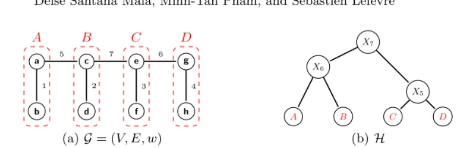
A B C D a b c d e f g h 1 2 3 4 5 7 6 (a) G = (V, E, w) A B C D X6 X5 X7 (b) H
Fig. 1. (a): A weighted graph G = (V, E, w). (b): A tree representation of the hierar-chical watershed H of G for the sequence (C, A, B, D) of minima of G.
2
Background notions
In this section, we first review graphs and hierarchical watersheds. Then, we review the literature on the use of prior knowledge and markers in the field of image processing. Finally, we recall the definition of Attribute Profile (AP). 2.1 Graphs and hierarchical watersheds
Watershed segmentation was proposed in the late 70’s and, since then, this con-cept has been extended to several frameworks and implemented through a variety of algorithms. The intuition behind the various definitions of the watershed seg-mentation derive from the topographic definition of watersheds: dividing lines between catchment basins, which are, in their turn, areas where collected pre-cipitation flows into the same regional minimum. These notions can be extended to gray-scale images and graphs, leading to different definitions of watershed segmentation. In this paper, we focus on watershed-cuts and hierarchical water-sheds defined in the context of edge-weighted graphs, as formalized in [5,6]. In the remainder of this section, we present the notions of graphs, hierarchies of partitions and hierarchical watersheds.
A (edge) weighted graph is a triplet G = (V, E, w) where V is a finite set, E is a subset of V × V , and w is a map from E into R. The elements of V and E are called vertices and edges (of G), respectively. Let G = (V, E, w) be a weighted graph and let G0= (V0, E0, w) be a graph such that V0⊆ V and E0 ⊆ E. We say that G0is a subgraph of G. A sequence π = (x0, . . . , xn) of vertices in V0is a path (in G0) from x0 to xn if {xi−1, xi} is an edge of G0 for any 1 ≤ i ≤ n. If x0= xn and if there are no repeated edges in π, we say that π is a cycle (in G0). The subgraph G0 of G is said to be connected if, for any x and x0 in V0, there exists a path from x to x0. Moreover, we say that G0 is a connected component of G if:
1. for any x and x0 in V0, if {x, x0} ∈ E then {x, x0} ∈ E0; and 2. there is no edge e = {y, y0} ∈ E such that y ∈ V \ V0 and y0∈ V0.
Let G = (V, E, w) be a graph and let G0= (V0, E0, w) be a connected subgraph of G. If the weight of any edge in E0 is equal to a constant k and if w(e) > k for any edge e = {x, y} such that x ∈ V0 and y ∈ V \ V0, then G0 is a (local) minimum of G.
For instance, Figure 1(a) illustrates a weighted graph with four minima de-limited by the dashed lines.
Important remark: in the remainder of this section, G = (V, E, w) denotes a connected weighted graph and n denotes the number of minima of G.
Let G0= (V0, E0, w) be a subgraph of G. A Minimum Spanning Forest (MSF) of G rooted in G0 is a subgraph G00= (V, E00, w) of G such that:
1. for every connected component X00 of G00, there is exactly one connected component X0 of G0 such that X0 is a subgraph of X00;
2. every cycle in G00 is a cycle in G0; and 3. P
e∈E00w(e) is minimal among all graphs which satisfy conditions (1) and (2).
A partition of V is a set P of disjoint subsets of V such that the union of the elements in P is V . The partition of V induced by a graph G0 is the partition P such that every element of P is the set of vertices of a connected component of G0. A hierarchy of partitions of V is a sequence H = (P0, . . . , Pn) of partitions of V such that Pn = {V } and such that, for any 0 < i ≤ n, every element of Pi is the union of elements of Pi−1.
Any hierarchy of partitions H can be represented as a tree whose vertices correspond to the regions of H and whose edges link nested regions. For instance, Figure 1(b) shows a tree representation of the hierarchy H = (P0, P1, P2, P3), where P0= {{a, b}, {c, d}, {e, f }, {g, h}}, P1= {{a, b}, {c, d}, {e, f, g, h}}, P2= {{a, b, c, d}, {e, f, g, h}} and P3= {{a, b, c, d, e, f, g, h}}.
Let S = (M1, . . . , Mn) be a sequence of n distinct minima of G such that, for any 0 < i ≤ n, we have Mi = (Vi, Ei, w). The hierarchy of Minimum Spanning Forests of G for S, also known as hierarchical watershed of G for S, is a hierarchy H = (P1, . . . , Pn) of partitions of V such that each partition Pi is the partition induced by the MSF of G rooted in the graph (S
j≥i Vj, S
j≥i Ej, w). A hierarchical watershed of the graph G of Figure 1(a) for the sequence (C, A, B, D) of minima of G is illustrated in Figure 1(b).
2.2 Prior knowledge for image processing
Unsupervised data pre-processing methods, such as watershed segmentation and image filtering (e.g. Sobel, Laplacian and morphological filters), are successfully employed in several computer vision tasks, including classification and detec-tion problems. Moreover, when prior knowledge is provided, this can be used to provide further improvements.
In the context of image segmentation, a widespread method to introduce prior knowledge in the results is to consider user-defined markers, which are subsets of image pixels indicating the locations of objects of interest. Such markers guide the segmentation algorithm and assure that the objects of interest are segmented into distinct regions. The notion of markers has been especially explored in wa-tershed segmentations, in which catchment basins are grown from input markers instead of the regional minima of an image (or graph) [2].
The use of markers in a watershed segmentation can go beyond the intro-duction of new regional minima. The values or spectral signatures of the marked pixels can provide further knowledge about the objects we aim to segment. For instance, in [10,11], the authors use the spectral signature of training samples in the construction of watershed segmentations of multi-spectral images. First, the spectral signature of training pixels is used to train a classifier, which is then ap-plied on the whole image and used to obtain a probability map per class. Then, those maps are combined and used to obtain a single watershed segmentation. Another use of supervised classification for watersheds has been proposed in [15], where the watershed segmentation is computed from user-defined markers com-bined with probability maps computed for each targeted class. More precisely, catchment basins are grown from different markers, and the probability maps, combined with the original data, are used simultaneously in the process. In re-mote sensing, the later approach has been applied to the detection of buildings [1] and shorelines [17] in multi-spectral images. Finally, in [9], prior knowledge from markers is employed on several interactive image segmentation methods, includ-ing watersheds, in the framework of edge-weighted graphs. Edge weights are defined as a linear combination of the weights obtained from two sources: from the pixel values and from the classification probability maps computed from the markers that are incrementally provided by the users.
More generally, knowledge from markers can be used by other kinds of pre-processing methods beyond watershed segmentation. Namely, spectral signatures of training pixels have been used in [4] to optimize the data pre-processing with alternating sequential filters. Hence, training pixels are used for pre-processing the input data, as well as for the final pixel classification. A related approach is proposed in [23], where training pixels are used to optimize vector orderings for morphological operations applied to hyperspectral images.
In the context of hierarchical segmentation, prior knowledge can play a role in defining which regions should be highlighted at different levels of a hierarchy. In [21], a marker-based hierarchical segmentation is proposed for hyperspectral image classification. Labeled markers are derived from a probability classifica-tion map, which is obtained from training samples, as done in [10,11,15]. Then, those labeled markers guide the construction of a hierarchical segmentation by preventing regions of different classes to be merged, and by propagating the la-beled markers to unlala-beled regions. Another related approach, proposed in [12], uses prior knowledge to keep the regions of interest from being merged early in the hierarchy, i.e., the details in the regions of interest are preserved at high levels of the hierarchy.
Finally, in [16], the authors propose a knowledge-based hierarchical repre-sentation for hyperspectral images. In their approach, a dissimilarity measure learned from training pixels is employed in the construction of α-trees.
2.3 Attribute profiles
Attribute profile (AP) [8] is a multilevel feature extraction method commonly applied to the analysis of remote sensing images. To convey spatial-spectral
features of remote sensing images, APs were initially defined as sequences of filtering operators on the max- and min-trees computed from the original data. Let X : P → Z, P ⊆ Z2 be a gray-scale image. The calculation of APs on X is achieved by applying a sequence of attribute filters based on a min-tree (i.e. attribute thickening operators {φA
k}Kk=1) and on a max-tree (i.e. attribute thinning operators {γA k}Kk=1) as follows: (X) =nφAK(X), φAK−1(X), . . . , φA1(X), X, γ1A(X), . . . , γ A K−1(X), γ A K(X) o , (1) where φA
k and γkA are respectively the thickening and thinning operators with respect to the attribute A and to the threshold k, and K is the number of selected thresholds. More precisely, the thickening φA
k(X) of X (resp. thinning γkA(X) of X) with respect to an attribute A and to a threshold k is obtained as follows: given the min-tree T (resp. max-tree T ) of X, the A attribute values (e.g. area, circularity and contrast) of the nodes of T are computed. If the attribute A is increasing, the nodes whose attribute values are inferior to k are pruned from the tree T ; otherwise other pruning strategies can be adopted [18]. Finally, the resulting image is reconstructed by projecting the gray levels of the remaining nodes of T into the pixels of X.
Since its appearance, the notion of APs has been extended to other hierarchi-cal representations including tree-of-shapes [7] and partition trees such as α-tree and ω-tree [3]. To obtain a profile from a partition tree instead of a component tree, some adaptations have to be made to the original definition of APs, as discussed in [3]. For instance, the nodes of a partition tree are not naturally associated to gray-level values, as it is the case of component trees. The strategy adopted in [3] is to represent each node as its level in the tree or as the maximum, minimum, or average gray-level of the leaf nodes (pixels) of this node. For more details about APs’ extensions, we invite readers to refer to a recent survey [18].
3
Watershed-based attribute profiles
In this article, we extend the notion of AP to hierarchical watershed obtained in the framework of edge-weighted graphs.
As mentioned in section 2.1, hierarchies of partitions, such as hierarchical watersheds, can be equally represented a (partition) tree. Hence, the filtering strategy of Watershed-APs is similar to the strategy described in [3] for the α-and ω-APs.
As discussed in [3], image reconstruction from partition trees is not straight-forward as it is from component trees. For node representation, we adopt one of the solutions proposed in [3] and already mentioned in section 2.3, in which a node is represented by the average gray-level of the pixels belonging to it. We highlight that, in the case of multiband images, the average grey level computed on each band might lead to spectral values not present in the input image. How-ever, in the context of attribute profiles used for pixel classification, our aim is
not image filtering. Hence, the fact that new spectral values (a.k.a. false colors) are created is not a problem as long as they allow us to distinguish between different semantic classes.
Note that hierarchical watersheds are usually constructed from a gradient of the original image, which contains more information about the contours between salient regions than about the spectral signature of those regions. Hence, we consider the original pixel values to obtain the nodes representation instead of the image gradient.
Formally, let X : P → Z be a gray-scale image and let G = (V, E, w) be a weighted graph which represents a gradient of X, i.e., V = P and, for every edge e = {x, y} in E, the weight w(e) represents the dissimilarity between x and y, e.g. w(e) = |X(x) − X(y)|. Let S be a sequence of minima of G ordered according to a given criterion C, and let H be the hierarchical watershed of G for the sequence S. Given the tree representation T of H, a Watershed-AP of X for the criterion C is constructed as a sequence of image reconstructions from filtered versions of T .
As discussed in section 2.2, user-defined markers and prior knowledge can boost the performance of watershed segmentations. In this article, we extend the use of prior knowledge to hierarchical watersheds. More specifically, we aim to enforce regional minima at the regions with high probability of belonging to any given ground-truth class. This is done through a combination of the methods proposed in [10,11,15]. Given a dataset I (e.g. a panchromatic or a RGB image) and its training set composed of c classes, we compute its hierarchical watershed using prior knowledge as follows:
1. Train a classifier using the training set of I and compute per-pixel classifi-cation probabilities (p1, . . . , pc) for all pixels of I;
2. Combine the classification probabilities into a single map µ : X → [0, 1] such that, for any pixel x in X, µ(x) = 1 −pp1(x)2+ . . . pc(x)2
3. Compute a 4- or 8-connected weighted graph GP = (V, E, wP) from µ such that, for any edge e = (x, y) in E, we have wP(e) = max(µ(x), µ(y)); 4. Compute a 4- or 8- connected weighted graph GG = (V, E, wG) which
rep-resents a gradient of I. For instance, for any edge e = (x, y) in E, we may have wG(e) = |I(x) − I(y)| or wG(e) = (I(x) − I(y))2;
5. Combine the weight maps wP and wG into a map wGP such that, for any edge e in E, we have wGP = wP(e) × wG(e); and
6. Finally, compute the hierarchical watershed of GGP = (V, E, wGP) for a given sequence of minima of G.
In the first step of our method, we are aware that: (1) there might be sample pixels of a given class whose spectral values are not represented in the training set, and (2) there might be pixels in the training set with very similar spectral signatures but which belong to distinct classes. In those cases, we expect the classifier to assign low classification probabilities to such pixels. This means that the watershed segmentation at those regions will be mostly guided by the original gray-levels of the image gradient. Then, in the second step of our method, we
combine the classification probability maps into a single probability map µ. We expect this combination to provide flat zones of pixels with high probability of belonging to any given class, i.e., subsets of pixels that should be merged early in the resulting hierarchical watershed. In the extreme case where the classifier assigns very high classification probabilities to all pixels of I, we would have a single flat zone and, consequently, a hierarchy with a single segmentation level. However, in that case, we might not need APs to improve the classification results on the image I. In the third step, a weighted graph (V, E, wP) is obtained from the combined probability map µ. Our choice for computing edge weights as the maximum between the probability values of neighbouring pixels was actually heuristic and was based on a few experiments with the datasets described in the next section. In the steps 4 and 5, a gradient (V, E, wG) of I is computed and then combined with (V, E, wP) as a multiplication of edge weights, similarly to [15]. We note that the proposed method is related to ones introduced in [12,16], the main difference being the type of hierarchy under consideration and how the original data is combined with the prior knowledge.
In Figure 2, we show that the proposed method can be effectively used to highlight objects of interest (e.g. cars) in hierarchical watersheds. Given the RGB image I of Figure 2(a) and the set of labeled training samples for the car (in blue) and background (in red) classes of Figure 2(b), we compute the probability map per class and combine them into the map µ of Figure 2(c), in which dark regions are composed of pixels with high probability of belonging to any given class. Then, the weighted graph GP = (V, E, wP) is computed from µ as described in the third step of our method. Next, we compute the gradient GG= (V, E, wG) of the Red channel of I such that, for any edge e = (x, y) in E, we have wG(e) = |I(x) − I(y)|. At this step, the Green and Blue channels could have been chosen and other dissimilarity measures could be used as well. Then, the weight maps wP and wG are combined into wP G as described previously. Finally, to compare the hierarchies obtained with and without prior-knowledge, we computed the area-based hierarchical watersheds H and H0 of GG and GGP, respectively. In Figures 2(d), (e) and (f), we show the reconstructions of the tree representation of H after filtering the nodes with area inferior to 100, 500 and 1000, respectively. Those reconstructions are represented with random colors. Similarly, Figures 2(g), (h) and (i) show the reconstructions performed on the tree representation of H0 for the same filterings. We observe that, by imposing regional minima at the location of the cars, we make those objects to appear earlier in the hierarchy H0 when compared to H and, at the same time, to be merged later to their surrounding regions. For instance, the dark blue car on the top left appears as a single region in all reconstructions performed on the tree representation of H0, which is not the case of H.
4
Experimental results
In this section, we evaluate the performance of Watershed-AP (computed with and without prior-knowledge) in the context of land-cover classification of remote
(a) (b) (c)
(d) (e) (f)
(g) (h) (i)
Fig. 2. (a): original image I. (b) training samples in red (background) and blue (cars). (c) classification probability map µ. (d), (e) and (f): image reconstructions obtained from a hierarchical watershed of I, by filtering the nodes with area inferior to 1000, 5000 and 10000, respectively. (g), (h) and (i): image reconstructions obtained from a hierarchical watershed of the combination of I and µ, by filtering the nodes with area inferior to 1000, 5000 and 10000, respectively.
sensing images. We first describe the panchromatic and RGB images considered in our study, as well as the experimental settings used for evaluation. Finally, we show that Watershed-AP outperforms AP and its variants including SDAP [7], α-AP [3] and ω-AP [3], on both datasets.
4.1 Datasets
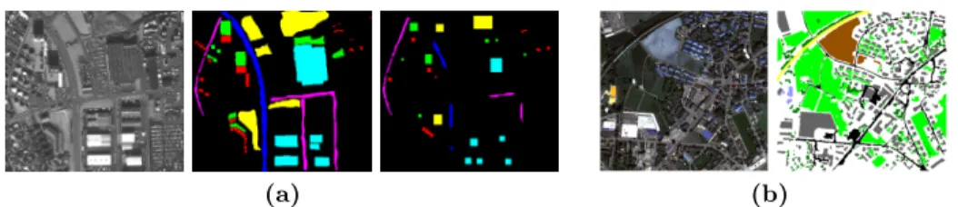
We validate our approach on two remote sensing datasets: the panchromatic Reykjavik dataset and a RGB image of Zurich dataset [24].
The Reykjavik dataset is a panchromatic image of size 628 × 700 pixels ac-quired by the IKONOS Earth imaging satellite with 1-m resolution in Reykjavik, Iceland. This data consists of six thematic classes including residential, soil, shadow, commercial, highway and road. The image was provided with already-split training and test sets (22741 training samples and 98726 test samples). The input image together with its thematic ground truth map are shown in Fig. 3(a). The Zurich Summer dataset [24] is a collection of 20 NIR+RGB images of various dimensions taken from a QuickBird acquisition of the city of Zurich, Switzerland, in August 2002. The ground-truth provided for each image consists of at most eight thematic classes: roads, buildings, trees, grass, bare soil, water, railways and swimming pools. In our experiments, we only consider the RGB channels of the first image zh1.tif of this dataset. The training set is composed of 1% of the labeled pixels randomly extracted for each class. The input image and its ground-truth are given in Fig. 3(b).
(a) (b)
Fig. 3. Two data sets used in our experimental study. (a) The 628 × 700 Reykjavik data. Left to right: panchromatic image, ground truth and training set including six thematic classes: residential, shadow, highway, soil, commercial, road. (b) The 610 × 340 Zurich data. Left to right: RGB image and ground truth including seven thematic classes: roads, buildings, trees, grass, bare soil, railways, swiming pools.
4.2 Experimental settings
AP and its variants were computed on the Reykjavik and Zurich datasets with the usual area and moment of inertia (MoI) attributes. The following ten area thresholds and four MoI thresholds were adopted for both datasets: λarea = {25, 100, 500, 1000, 5000, 10000, 20000, 50000, 100000, 150000} and λmoi = {0.2, 0.3, 0.4, 0.5}. For the Zurich dataset, the APs and their extensions are com-puted independently on each of the RGB bands and are concatenated, leading to Extended Attribute Profiles (EAP).
For each dataset I, hierarchical watersheds were computed from two 4-connected edge-weighted graphs: from the graph GG= (V, E, wG) obtained from a gradient of the original data I (without any prior-knowledge from markers), and the second one computed from the combination of the graph GG with the classification probability map obtained from the training set of I, as described in Section 3. For every edge e = (x, y) in E, we define wG(e) as |I(x) − I(y)|.
Supervised pixel classification was performed twice, once for obtaining the classification probability map and then to provide the final land-cover pixel clas-sification. Both were performed using a Random Forest classifier with 100 trees. The number of variables used for training was set to the square root of the feature vectors length. The different approaches are compared using the overall accuracy (OA), average accuracy per class (AA) and κ coefficient, as done in [8]. For each tested method, we report the average and standard deviation of the classification scores over ten runs.
As defined in section 2.1, hierarchical watersheds can be computed for any given ordering on the minima of a weighted graph. In our experiments, such orderings are obtained from extinction values [14,22] based on the area, dynamics and volume attributes.
5
Results and discussion
Tables 1-4 present the classification results of the Reykjavik and Zurich datasets. We compare the performance of the following methods: AP-maxT and AP-minT
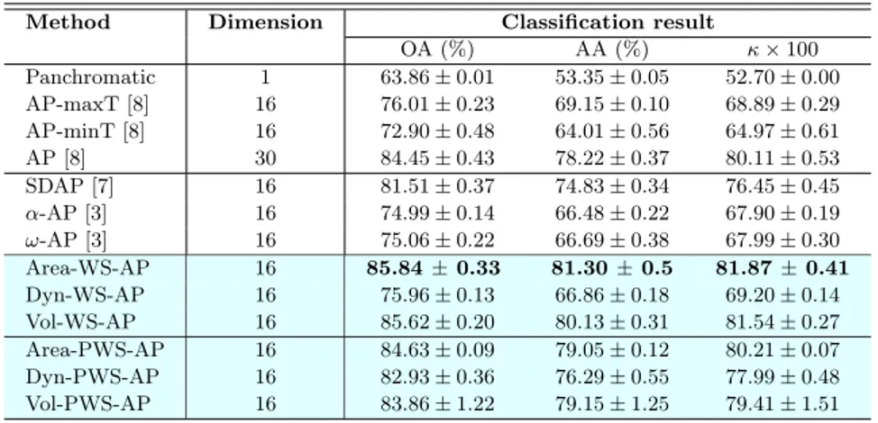
Table 1. Classification result of Reykjavik dataset obtained by different methods using the default 4-connectivity and 1-byte quantization.
Method Dimension Classification result
OA (%) AA (%) κ × 100 Panchromatic 1 63.86 ± 0.01 53.35 ± 0.05 52.70 ± 0.00 AP-maxT [8] 16 76.01 ± 0.23 69.15 ± 0.10 68.89 ± 0.29 AP-minT [8] 16 72.90 ± 0.48 64.01 ± 0.56 64.97 ± 0.61 AP [8] 30 84.45 ± 0.43 78.22 ± 0.37 80.11 ± 0.53 SDAP [7] 16 81.51 ± 0.37 74.83 ± 0.34 76.45 ± 0.45 α-AP [3] 16 74.99 ± 0.14 66.48 ± 0.22 67.90 ± 0.19 ω-AP [3] 16 75.06 ± 0.22 66.69 ± 0.38 67.99 ± 0.30 Area-WS-AP 16 85.84 ± 0.33 81.30 ± 0.5 81.87 ± 0.41 Dyn-WS-AP 16 75.96 ± 0.13 66.86 ± 0.18 69.20 ± 0.14 Vol-WS-AP 16 85.62 ± 0.20 80.13 ± 0.31 81.54 ± 0.27 Area-PWS-AP 16 84.63 ± 0.09 79.05 ± 0.12 80.21 ± 0.07 Dyn-PWS-AP 16 82.93 ± 0.36 76.29 ± 0.55 77.99 ± 0.48 Vol-PWS-AP 16 83.86 ± 1.22 79.15 ± 1.25 79.41 ± 1.51
obtained by filtering the max- and min-tree, respectively; AP [8], obtained as a concatenation of AP-maxT and AP-minT; SDAP [7]; α-AP and ω-AP [3]; and the Watershed-AP computed with and without prior knowledge. To simplify the notations, Watershed-AP computed without and with prior knowledge are denoted respectively as A-WS-AP and A-PWS-AP, where A is the attribute used in the construction of the hierarchical watersheds, namely Area, Dynamics (Dyn) and Volume (Vol).
For the Reykjavik dataset, Watershed-AP constructed with the area and vol-ume attributes outperform all other methods. As shown in Table 1, the best clas-sification result, obtained with Area-WS-AP, outperforms AP by 1.39%, 3.08% and 1.76% in terms or OA, AA and κ, respectively. Moreover, considering only the APs obtained from partition trees (α-AP, ω-AP and Watershed-AP), the Watershed-AP outperform both α- and ω-APs by more than 10% with respect to OA, AA and κ. In terms of classification results per class (see Table 2), the highest scores are achieved by Watershed-AP and AP, except for the shadow class, for which none of those methods where able to outperform the classifica-tion based only on panchromatic pixel values.
Let us now analyse the influence of the use of prior knowledge in the perfor-mance of Watershed-AP. For the Watershed-AP computed with the dynamics attribute, the use of prior knowledge led to an improvement of 6.97%, 9.43% and 8.79% in terms of OA, AA and κ, respectively, and better accuracy scores for all six semantic classes. Whereas, the same did not happen for the Watershed-AP computed with area and volume, for which the overall classification results decreased by more than 1%.
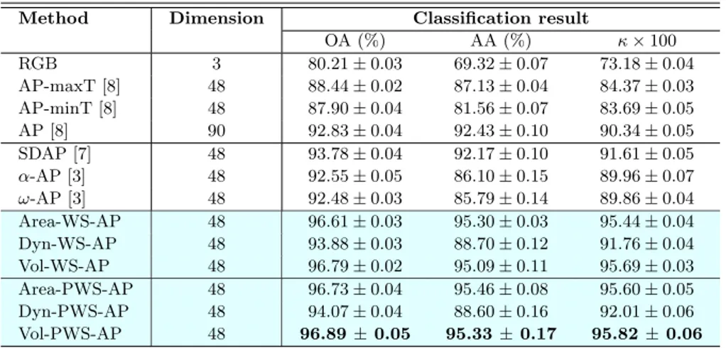
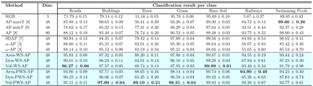
On the Zurich dataset, the Watershed-APs outperform all other methods (see Table 3). The best method, Vol-PWS-AP, outperforms SDAP by 3.11%, 3.16% and 4.21% in terms of OA, AA and κ, respectively. Similar to the Reyk-javik dataset, the Watershed-AP yielded the best results per class, except for the
Table 2. Classification result of Reykjavik dataset obtained by different methods using the default 4-connectivity and 1-byte quantization.
Method Dim. Classification results per class
Residential Soil Shadow Commercial Highway Road Panchromatic 1 6.02 ± 0.36 73.81 ± 0.00 90.94 ± 0.01 77.86 ± 0.09 16.60 ± 0.00 54.87 ± 0.01 AP-maxT [8] 16 44.55 ± 0.42 79.64 ± 1.29 88.28 ± 0.01 88.41 ± 1.51 51.15 ± 0.15 62.88 ± 0.18 AP-minT [8] 16 30.79 ± 0.68 85.55 ± 0.22 81.04 ± 0.73 81.89 ± 0.16 39.93 ± 6.37 64.89 ± 3.42 AP [8] 30 62.11 ± 0.57 91.29 ± 1.52 76.58 ± 1.61 92.79 ± 0.36 74.45 ± 0.32 72.08 ± 0.27 SDAP [7] 16 56.73 ± 1.11 89.57 ± 1.17 78.50 ± 0.89 90.45 ± 0.12 62.77 ± 0.24 70.94 ± 1.20 α-AP [3] 16 45.68 ± 1.33 88.45 ± 0.39 81.40 ± 0.08 82.11 ± 0.05 69.34 ± 0.37 31.93 ± 0.58 ω-AP [3] 16 47.15 ± 1.24 88.60 ± 0.38 81.39 ± 0.06 82.02 ± 0.16 69.20 ± 0.31 31.75 ± 1.66 Area-WS-AP 16 79.23 ± 1.39 94.98 ± 0.28 87.38 ± 0.66 89.33 ± 0.08 87.99 ± 1.52 48.88 ± 1.65 Dyn-WS-AP 16 47.16 ± 1.08 89.74 ± 0.15 80.26 ± 0.16 84.47 ± 0.48 71.68 ± 0.19 27.85 ± 0.41 Vol-WS-AP 16 74.41 ± 0.82 95.98 ± 0.19 84.00 ± 0.70 89.85 ± 0.04 87.62 ± 1.33 48.90 ± 2.07 Area-PWS-AP 16 71.05 ± 0.11 91.08 ± 0.08 80.67 ± 0.50 91.90 ± 0.13 88.09 ± 0.00 51.54 ± 0.34 Dyn-PWS-AP 16 65.70 ± 1.17 94.87 ± 0.23 80.81 ± 0.67 88.55 ± 0.22 77.99 ± 0.19 49.84 ± 3.51 Vol-PWS-AP 16 75.05 ± 0.16 89.91 ± 3.24 79.50 ± 0.45 90.27 ± 0.16 84.89 ± 3.37 55.29 ± 5.31
Table 3. Classification result of Zurich dataset obtained by different methods using the default 4-connectivity and 1-byte quantization.
Method Dimension Classification result
OA (%) AA (%) κ × 100 RGB 3 80.21 ± 0.03 69.32 ± 0.07 73.18 ± 0.04 AP-maxT [8] 48 88.44 ± 0.02 87.13 ± 0.04 84.37 ± 0.03 AP-minT [8] 48 87.90 ± 0.04 81.56 ± 0.07 83.69 ± 0.05 AP [8] 90 92.83 ± 0.04 92.43 ± 0.10 90.34 ± 0.05 SDAP [7] 48 93.78 ± 0.04 92.17 ± 0.10 91.61 ± 0.05 α-AP [3] 48 92.55 ± 0.05 86.10 ± 0.15 89.96 ± 0.07 ω-AP [3] 48 92.48 ± 0.03 85.79 ± 0.14 89.86 ± 0.04 Area-WS-AP 48 96.61 ± 0.03 95.30 ± 0.03 95.44 ± 0.04 Dyn-WS-AP 48 93.88 ± 0.03 88.70 ± 0.12 91.76 ± 0.04 Vol-WS-AP 48 96.79 ± 0.02 95.09 ± 0.11 95.69 ± 0.03 Area-PWS-AP 48 96.73 ± 0.04 95.46 ± 0.08 95.60 ± 0.05 Dyn-PWS-AP 48 94.07 ± 0.04 88.60 ± 0.16 92.01 ± 0.06 Vol-PWS-AP 48 96.89 ± 0.05 95.33 ± 0.17 95.82 ± 0.06
‘swimming pools’ class (see Table 4). Moreover, on this dataset, the use of prior knowledge in the construction of hierarchical watersheds led to small improve-ments for all three Watershed APs. More precisely, we observed an improvement of up to 0.25% in terms of OA, AA and κ for the Watershed-APs constructed with the area, dynamics, and volume attributes.
6
Conclusion
We proposed the Watershed-AP as an extension of AP to hierarchical water-sheds computed from (edge) weighted graphs. Besides, we investigate the rele-vance of using semantic prior knowledge in the construction of such hierarchies. We validated our approach on the pixel classification of two remote sensing im-ages, which showed the potential of hierarchical watersheds in this field. On both datasets, Watershed-APs, computed with and without prior-knowledge, presented the highest evaluation scores when compared to the standard APs.
Table 4. Classification result of Zurich dataset obtained by different methods using the default 4-connectivity and 1-byte quantization.
Method Dim. Classification result per class
Roads Buildings Trees Grass Bare Soil Railways Swimming Pools RGB 3 71.79 ± 0.15 79.14 ± 0.12 51.16 ± 0.19 91.76 ± 0.06 95.69 ± 0.10 5.87 ± 0.37 89.85 ± 0.43 AP-maxT [8] 48 85.88 ± 0.12 90.65 ± 0.09 56.41 ± 0.20 93.26 ± 0.07 99.30 ± 0.03 84.72 ± 0.14 99.66 ± 0.26 AP-minT [8] 48 78.62 ± 0.17 85.22 ± 0.13 77.31 ± 0.20 96.29 ± 0.04 97.64 ± 0.05 43.51 ± 0.44 92.37 ± 0.28 AP [8] 90 88.12 ± 0.19 93.49 ± 0.07 76.74 ± 0.20 96.53 ± 0.05 99.48 ± 0.02 93.75 ± 0.23 98.90 ± 0.43 SDAP [7] 48 90.94 ± 0.12 94.35 ± 0.07 79.42 ± 0.14 97.09 ± 0.04 99.56 ± 0.01 84.94 ± 0.54 98.92 ± 0.41 α-AP [3] 48 88.00 ± 0.11 95.25 ± 0.07 82.01 ± 0.26 95.30 ± 0.05 98.64 ± 0.03 58.07 ± 0.83 85.42 ± 0.46 ω-AP [3] 48 88.14 ± 0.10 95.12 ± 0.06 82.19 ± 0.34 95.21 ± 0.04 98.68 ± 0.04 55.65 ± 0.60 85.53 ± 0.70 Area-WS-AP 48 95.83 ± 0.08 97.32 ± 0.05 88.20 ± 0.11 97.88 ± 0.04 99.87 ± 0.01 94.55 ± 0.19 93.44 ± 0.24 Dyn-WS-AP 48 90.01 ± 0.10 96.24 ± 0.11 84.01 ± 0.14 96.18 ± 0.05 99.28 ± 0.03 67.94 ± 0.61 87.25 ± 0.50 Vol-WS-AP 48 96.27 ± 0.06 97.57 ± 0.05 88.74 ± 0.13 97.95 ± 0.03 99.89 ± 0.01 93.40 ± 0.34 91.79 ± 0.98 Area-PWS-AP 48 94.86 ± 0.09 97.71 ± 0.05 88.65 ± 0.16 98.14 ± 0.04 99.74 ± 0.06 94.90 ± 0.40 94.23 ± 0.40 Dyn-PWS-AP 48 90.23 ± 0.14 96.06 ± 0.07 85.25 ± 0.20 96.58 ± 0.04 99.22 ± 0.05 65.26 ± 0.63 87.64 ± 0.74 Vol-PWS-AP 48 95.11 ± 0.11 97.90 ± 0.04 89.10 ± 0.21 98.31 ± 0.04 99.82 ± 0.02 93.28 ± 0.67 93.77 ± 0.81
As future work, we will to explore the versatility of hierarchical watersheds by considering other methods to obtain the gradient of remote sensing images, as well as different ways of including prior knowledge in the computation of those hierarchies. We are also interested in theoretical properties of the Watershed-AP, namely its link with other related methods such as Feature Profiles [19] and Extinction Profiles [13].
7
Acknowledgements
This work was partially supported by the ANR Multiscale project under the reference ANR-18-CE23-0022. The authors would like to thank Prof. Jon Atli Benediktsson for making available the Reykjavik image.
References
1. Aksoy, S., et al.: Performance evaluation of building detection and digital surface model extraction algorithms: Outcomes of the PRRS 2008 algorithm performance contest. In: PRRS 2008. pp. 1–12. IEEE (2008)
2. Beucher, S., Meyer, F.: The morphological approach to segmentation: the water-shed transformation. Mathematical Morphology in Image Processing 34, 433–481 (1993)
3. Bosilj, P., Damodaran, B.B., Aptoula, E., Dalla Mura, M., Lef`evre, S.: Attribute profiles from partitioning trees. In: ISMM. pp. 381–392 (2017)
4. Courty, N., Aptoula, E., Lef`evre, S.: A classwise supervised ordering approach for morphology based hyperspectral image classification. In: ICPR2012. pp. 1997– 2000. IEEE (2012)
5. Cousty, J., Bertrand, G., Najman, L., Couprie, M.: Watershed cuts: Minimum spanning forests and the drop of water principle. IEEE PAMI 31(8), 1362–1374 (2008)
6. Cousty, J., Najman, L., Perret, B.: Constructive links between some morphological hierarchies on edge-weighted graphs. In: ISMM. pp. 86–97. Springer (2013) 7. Dalla Mura, M., Benediktsson, J., Bruzzone, L.: Self-dual attribute profiles for the
8. Dalla Mura, M., Benediktsson, J.A., Waske, B., Bruzzone, L.: Morphological at-tribute profiles for the analysis of very high resolution images. IEEE TGRS 48(10), 3747–3762 (2010)
9. De Miranda, P.A., Falc˜ao, A.X., Udupa, J.K.: Synergistic arc-weight estimation for interactive image segmentation using graphs. Computer Vision and Image Un-derstanding 114(1), 85–99 (2010)
10. Derivaux, S., Forestier, G., Wemmert, C., Lef`evre, S.: Supervised image segmenta-tion using watershed transform, fuzzy classificasegmenta-tion and evolusegmenta-tionary computasegmenta-tion. PRL 31(15), 2364–2374 (2010)
11. Derivaux, S., Lefevre, S., Wemmert, C., Korczak, J.: Watershed segmentation of remotely sensed images based on a supervised fuzzy pixel classification. In: IEEE IGARSS. pp. 3712–3715 (2006)
12. Fehri, A., Velasco-Forero, S., Meyer, F.: Prior-based hierarchical segmentation highlighting structures of interest. Mathematical Morphology-Theory and Appli-cations 3(1), 29–44 (2019)
13. Ghamisi, P., Souza, R., Benediktsson, J.A., Zhu, X.X., Rittner, L., Lotufo, R.A.: Extinction profiles for the classification of remote sensing data. IEEE Transactions on Geoscience and Remote Sensing 54(10), 5631–5645 (2016)
14. Grimaud, M.: New measure of contrast: the dynamics. In: Image Algebra and Morphological Image Processing III. vol. 1769, pp. 292–305. International Society for Optics and Photonics (1992)
15. Lef`evre, S.: Knowledge from markers in watershed segmentation. In: CAIP. pp. 579–586. Springer (2007)
16. Lef`evre, S., Chapel, L., Merciol, F.: Hyperspectral image classification from mul-tiscale description with constrained connectivity and metric learning. In: 2014 WHISPERS. pp. 1–4. IEEE (2014)
17. Lefevre, S., Puissant, A., Levoy, F.: Weakly supervised image segmentation: ap-plication to mapping and monitoring of salt marsh vegetation in the mont-saint-michel bay from high resolution imagery. In: ESA-EUSC-JRC 2011. pp. 4–p (2011) 18. Maia, D.S., Pham, M.T., Aptoula, E., Guiotte, F., Lef`evre, S.: Classification of remote sensing data with morphological attributes profiles: A decade of advances. IEEE GRSM (2021)
19. Pham, M.T., Aptoula, E., Lef`evre, S.: Feature profiles from attribute filtering for classification of remote sensing images. IEEE Journal of Selected Topics in Applied Earth Observations and Remote Sensing 11(1), 249–256 (2017)
20. Soille, P., Pesaresi, M.: Advances in mathematical morphology applied to geo-science and remote sensing. IEEE TGRS 40(9), 2042–2055 (2002)
21. Tarabalka, Y., Tilton, J.C., Benediktsson, J.A., Chanussot, J.: Marker-based hi-erarchical segmentation and classification approach for hyperspectral imagery. In: 2011 ICASSP. pp. 1089–1092. IEEE (2011)
22. Vachier, C., Meyer, F.: Extinction value: a new measurement of persistence. In: IEEE Workshop on Nonlinear Signal and Image Processing. vol. 1, pp. 254–257 (1995)
23. Velasco-Forero, S., Angulo, J.: Supervised ordering in Rp: Application to morpho-logical processing of hyperspectral images. IEEE TIP 20(11), 3301–3308 (2011) 24. Volpi, M., Ferrari, V.: Semantic segmentation of urban scenes by learning local
class interactions. In: Proceedings of the IEEE Conference on Computer Vision and Pattern Recognition Workshops. pp. 1–9 (2015)