HAL Id: hal-00867702
https://hal.archives-ouvertes.fr/hal-00867702
Submitted on 30 Sep 2013
HAL is a multi-disciplinary open access
archive for the deposit and dissemination of
sci-entific research documents, whether they are
pub-lished or not. The documents may come from
teaching and research institutions in France or
abroad, or from public or private research centers.
L’archive ouverte pluridisciplinaire HAL, est
destinée au dépôt et à la diffusion de documents
scientifiques de niveau recherche, publiés ou non,
émanant des établissements d’enseignement et de
recherche français ou étrangers, des laboratoires
publics ou privés.
Nonparametric time series modelling for industrial
prognostics and health management.
Ahmed Mosallam, Kamal Medjaher, Noureddine Zerhouni
To cite this version:
Ahmed Mosallam, Kamal Medjaher, Noureddine Zerhouni. Nonparametric time series modelling for
industrial prognostics and health management.. International Journal of Advanced Manufacturing
Technology, Springer Verlag, 2013, pp.1-25. �10.1007/s00170-013-5065-z�. �hal-00867702�
(will be inserted by the editor)
Nonparametric Time Series Modelling for Industrial
Prognostics and Health Management
Ahmed Mosallam · Kamal Medjaher and Noureddine Zerhouni
Received: date / Accepted: date
Abstract Prognostics and health management (PHM) methods aim at
de-tecting the degradation, diagnosing the faults and predicting the time at which a system or a component will no longer perform its desired function. PHM is based on access to a model of a system or a component using one or combi-nation of physical or data driven models. In physical based models one has to gather a lot of knowledge about the desired system, and then build analytical model of the system function of the degradation mechanism that is used as a reference during system operation. On the other hand data-driven models are based on the exploitation of symptoms or indicators of degradations using sta-tistical or Artificial Intelligence (AI) methods on the monitored system once it is operational and learn the normal behaviour.
Trend extraction is one of the methods used to extract important informa-tion contained in the sensory signals, which can be used for data driven mod-els. However, extraction of such information from collected data in a practical working environment is always a great challenge as sensory signals are usually multidimensional and obscured by noise. Also, the extracted trends should A. Mosallam FEMTO-ST Institute AS2M department 25000 Besan¸con, France. E-mail: Ahmed.Mosallam@femto-st.fr K. Medjaher FEMTO-ST Institute AS2M department 25000 Besan¸con, France. E-mail: Kamal.Medjaher@ens2m.fr N. Zerhouni FEMTO-ST Institute AS2M department 25000 Besan¸con, France. E-mail: Nourredine.Zerhouni@ens2m.fr
represent the nominal behaviour of the system as well as should represent the health status evolution.
This paper presents a method for nonparametric trend modelling from multidimensional sensory data so as to use such trends in machinery health prognostics. The goal of this work is to develop a method that can extract features representing the nominal behaviour of the monitored component and from these features extract smooth trends to represent the critical compo-nent’s health evolution over the time. The proposed method starts by multi-dimensional feature extraction from machinery sensory signals. Then, unsuper-vised feature selection on the features domain is applied without making any assumptions concerning the number of the extracted features. The selected features can be used to represent the nominal behaviour of the system and hence detect any deviation. Then, empirical mode decomposition algorithm (EMD) is applied on the projected features with the purpose of following the evolution of data in a compact representation over time. Finally, ridge regres-sion is applied to the extracted trend for modelling and can be used later for remaining useful life prediction.
The method is demonstrated on accelerated degradation dataset of bear-ings acquired from PRONOSTIA experimental platform and another dataset downloaded form NASA repository where it is shown to be able to extract signal trends.
Keywords Feature Extraction · Health Indicator · Trend Construction ·
Health State Detection · Prognostics
1 Introduction
The degradation of machine critical components is one of the main reasons of machines breakdown. Moreover, faulty components can also affect other components in the system which might lead to sever consequences. Effec-tive condition monitoring and health assessment of machinery deterioration is therefore crucial for reducing the downtime and the costs while increasing the availability [20].
Maintenance strategies can be classified into 1) Breakdown maintenance, 2) Preventive maintenance and 3) Condition-based maintenance (CBM) [16]. In breakdown maintenance no actions are taken to maintain the equipment until it breaks down. Preventive maintenance only includes setting periodic intervals for machine inspection. CBM analyses the condition measurements that do not interrupt normal operations. Compared to other maintenance strategies, CBM attempts to avoid unnecessary tasks by taking actions only when there is evidence of abnormal behaviour in the machine. Thus, CBM can produce significant saving through more convenient scheduling and therefore has been widely explored in research and industry lately [36].
One of the most important CBM activities is prognostics and health man-agement (PHM) which can be defined as the process of detecting abnormal conditions, diagnosis of the fault and their cause and prognostics of future
fault progression, see [12] [31]. PHM research has been shifting lately from fault detection and diagnostics to prognostics. Prognostics can be defined as the estimation of time to failure and risk for one or more existing or future fail-ure modes [15]. It usually requires the past history of the machinery condition sensory data [34]. The machinery health progression can be then extracted from the acquired data. The extracted progression data are then used as input for prediction or estimation algorithms to predict the future machine status [22].
The process of extracting representative health progression data from sen-sory time series data is known as trend extraction [3]. It can be performed us-ing multiple parameters, where relations between parameters can be utilised to represent the deterioration. However, sensory signals usually contain tremen-dous amount of oscillations and partly or completely hidden by noise which can be very challenging to process and to extract informative representation of the machine status. Also, the extracted trends should be used as a reference for the nominal behaviour and to predict the health status in the future.
In this work, time and frequency domain features have been extracted from two sensory time series. The features have been grouped using unsupervised feature selection algorithm based on symmetrical uncertainty measure, which can be used as a reference model for the nominal behaviour. Then, each group of features has been projected into a compact two dimensional representation using principle component analysis (PCA) [19]. In order to get a monotonic like signals, the final trends were extracted from each projected group using empirical mode decomposition algorithm (EMD) [14] and used to build a re-gression model of the machinery health prore-gression. These models can be used later for predicting the remaining useful life of the system.
This paper is organised as follows. A detailed literature review is depicted in section 2. Section 3 explains the method in details. The experimental results are shown in the section 4. Finally, a conclusion of the this paper and the future work is depicted in section 5.
2 Background
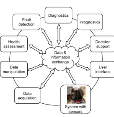
Data-driven PHM methods aim at building degradation models from sensory data acquired from sensors attached to critical components, see Figure 1. These sensory data contain valuable information about several aspects of health pro-gression, which has proved to be very challengeable. In this section we review state of the art of preprocessing approaches for the main PHM activities.
2.1 Fault detection
Fault or anomaly detection is the simplest part of PHM; which can be defined as the process of identifying when a fault/outlier has occurred. This section is dedicated to review some of the research work conducted for this task.
Data & information exchange Data acquisition Diagnostics Prognostics Data manipulation Health assessment Decision support User interface System with sensors Fault detection
Fig. 1: PHM General Scheme
An online anomaly detection algorithm that is not based on any learning algorithm has been proposed in [8]. The algorithm sets different operation modes once it starts running on N observations. Any change on the number of the clusters or the behaviour of the new data in an already defined cluster will be considered as suspicious behaviour. The proposed method is divided into two main parts, Initialisation and Monitoring. For initialisation 27 features were extracted, however, the authors did not specify exactly all the features. Then, data standardisation has been performed by applying unit variance and mean centering. PCA has been used for data dimensionality reduction. Fi-nally estimating the unknown numbers of operating modes clusters (OM), by using greedy expectation maximisation clustering algorithm. For monitoring part, first feature extraction has been applied. Then calculating of the online data and updating the modelled mean and variance of the old dataset have been performed. Data standardisation for the online readings was performed as in the initialisation part and also dimensionality reduction. Then updating OM clusters by using Mahalanobis distance measure. Finally, tracking OM by using evolving Takagi-Sugeno model in order to predict the dynamics of the data within each cluster. A comparison between PCA and partial least square (PLS) for fault detection has been presented in [33]. Moreover, the authors have used PLS for prognostics. The proposed method is divided into three parts, feature extraction, modelling and deviation detection. For feature extraction, 16 signals have been measured from moving gate-type incinera-tor. Building the model on healthy datasets using PCA and PLS. Finally, T square and Q statistics have been proposed to detect faults. The results show that both PCA and PLS performed fairly well in fault detection and PLS was also good for prognostics. An algorithm for machinery health monitoring and early fault detection has been proposed in [23]. The method decomposes the input signal into Intrinsic Mode Functions (IMFs) using Empirical Mode Decomposition (EMD), then Combined Mode Function (CMF) is applied to mix neighbouring IMFs to obtain the best signal. Feature extraction is then
performed using Fourier Transform (FT) on the acquired signal. Finally, the method uses Hidden Markov Models (HMMs) to build a model of the normal condition of the gearbox and Average Probability Index (API) is constructed as an index for machinery health status. A visual tool for fault detection and monitoring temporal evolution of aircraft engines health is presented in [7]. The environmental variables and engine effects are removed from rough mea-surements using General Linear Model (GLM). The residuals of the regression are used after that for training Self Organised Maps (SOMs) which shows the evolution of the motor status. Two methods for detecting anomalies in time series datasets acquired from different machinery sensors have been proposed in [1]. The first approach uses entropy analysis over the entire set of sensors at once to detect anomalies that have broad system-wide impact. It starts by smoothing and normalising time-series data for each sensor. Then, sampling the time-series values using uniformly sized bins. Finally, Shannon Entropy is computed for each time step as a reference model for the system. The second approach uses automated clustering of sensors combined with intra-cluster en-tropy analysis to detect anomalies and faults that have more local impact. For each of the n sensors, the method computes the Pearson correlation between each pair of sensors and form an n by n distance matrix. Then, the method clusters the sensors by performing a graph-partitioning of the adjacency graph and performs a time-windowed correlation within each sensor cluster. Finally, the entropy of the m discrete values has been computed to provide the cluster entropy for the system. The strength points in this work were no parameters to tune and it is easy to implement. However, the entropy does not differentiate between anomalies or noise which make it difficult for the method to detect different types of faults. A method for fault detection for electrical machines has been proposed in [32]. The method learns the normal behaviour over the time and detects any changes between the signals due to degradation of the system. The proposed method selects interesting features from the measured signals from the system using pairwise similarity measure algorithm and uses Gaussian Mixture Models (GMM) for relation description. Finally, a distance measure between different signals was calculated as indicator for the system deviation. A method for unsupervised change detection and health monitoring for Diesel engines has been proposed in [28]. The method is based on building a model using Independent Component Analysis (ICA). Probabilistic outlier detection algorithm has been also proposed for anomalies detection.
2.2 Diagnostics
Another important aspect in PHM systems is diagnostics and evaluation of wear advancements and it is presented in this section. A multidimensional diagnostics approach for mechanical systems has been presented in [4]. Vibra-tion signals were acquired from diesel engine, heavy fan and rubbing blades in a turbo-set to validate the approach. The authors applied mean centering and normalisation for the signals and then using Singular Value
Decomposi-tion (SVD), the multidimensional dataset were reduced to a lower dimension. Finally, health evolution indexing and fault diagnostics has been proposed by choosing the most informative SVD indexes. The same authors also proposed PCA instead of SVD for its computational efficiency in [5]. SOMs have been proposed in [25] for fault diagnostics and assessment of fault severity. Kurto-sis and line integral of acceleration signal have been extracted from bearings vibration signals for different faults. Then a SOM has been trained using the extracted features. Empirical Mode Decomposition (EMD) was also proposed in many works as it returns smooth monotonic like signals. A comparison study has been performed on the performance of 4 statistical indexes such as crest factor, kurtosis, skewness and beta distribution function [13]. The study shows that there is no significant advantage in using beta function com-pared to using kurtosis and crest factor for detecting and identifying different machinery defects. The paper also shows that the statistical parameters are affected by the shaft speed. The proposed method is only based on extract-ing four features mentioned earlier from vibration and sound signals acquired from test rig. Two temporal models, HMM and Auto regressive moving model with exogenous input (ARMAX) have been used for diagnostics in [10]. In this work 16 features have been extracted from force signals acquired from cutter milling machine. Selecting dominant features has been applied using
least multicollinearity along with a high R2. Finally, building models for
dif-ferent tool wears using ARMAX and HMM. A method for diagnostics and tool state recognition has been proposed in [18]. The method shows that using feature selection to select smaller set of features yield in more effective results. The proposed method is divided into three parts, feature extraction, feature selection and tool state learning. For feature extraction, 13 features have been extracted from acoustic emission (AE) signals acquired from CNC machine. Feature selection has been done using automatic relevance determination to select features which appear to have more potential use. Finally, the tool state learning has been conducted by Support Vector Machine (SVM). The perfor-mance of four classification algorithm for fault diagnostics has been compared in [9]. 16 features were extracted from force sensors attached to a cutting ma-chine. Then, 3 features were automatically selected from the extracted features using Genetic Algorithms (GA). A segmentation algorithm for health moni-toring and signal trending has been proposed in [6]. It is conducted in four steps: 1) On-line segmentation of data into linear segments, 2) Classification of the segmented lines into 7 shapes, 3) Transform the obtained shapes into three main shapes and 4) Aggregate of the current episode with the previous ones to form the signal trend. The performance of SVM versus ANN for gear fault diagnostics has been compared in [37]. The method is based on selecting important features from a larger features set and it shows that this selection increases the classification accuracy. Finally, the authors used datasets for 9 different gear fault classes. For each class 40 measures were recorded. The comparison shows that SVM outperforms Artificial Neural Network (ANN). An unsupervised feature selection method for deciding the optimal depth for Wavelet Packet Decomposition (WPD) has been presented in [35]. The paper
shows that using feature selection to determine the depth for WPD led to a model which can retain almost all the accuracy of models built using a much deeper transform. The proposed method determines the appropriate level us-ing Chi squared and information gain and then builds a diagnostics model using Naive Bayes Classifier. A method shows that if the size of the SOM is chosen judiciously then it is possible to monitor and identify different range of faults has been presented in [17]. The method proposes an empirically derived equation that governs the proper network size for efficient diagnostics.
2.3 Prognostics
Prognostics can be defined as the prediction of when a failure might take place. Prognostics has recently attracted a lot of research interest due to the need of models for accurate estimation of remaining useful life (RUL) for different applications.
A method for prognostics and health assessment has been proposed in [39]. The method starts by extracting 16 time and frequency features from double suction pump vibration signals. The method then uses PCA to merge features and to project the multidimensional features vector into a compact indicator. Finally, fault threshold has been calculated using Best Efficiency Point. Auto regression (AR) filter has been used to model vibration signal from bearing test rig in [21]. The model parameters have been estimated using Levinson-Durbin recursion (LDR). Then the energy ratio between the random parts and the original signal was used as fault indicator. The algorithm is simple to implement and suitable for highly accelerated signals. An integrated frame-work for fault detection, diagnosis and prognosis using Hidden markov model (HMM) has been presented in [40]. The proposed framework starts the data preprocessing by using frame blocking, frequency spectral analysis and noise filtering. Then using PCA the dimensionality of the dataset has been reduced. Next, the health status estimator has been built using HMM and health index interpolation by using Paris’s formula. A probabilistic model for online health indicator of bearing wear using wavelet package decomposition and HMM has been proposed in [27]. The method is divided into three parts, vibration signal
is divided into equal-sized signal epochs, nthlevel WPD was applied to these
signal epochs and finally the probabilities of the HMM for the normal condi-tion are calculated which can be used as the health indicator. The main con-tribution in this method was the proposition of a new probabilistic model for machinery health monitoring using HMM. A single hidden semi-markov model for prognostics has been proposed in [11]. In this work 7 signals, 3 force, 3 vi-bration and 1 acoustics have been acquired from CNC milling machine. Then 16 statistical features were extracted from the three force acquired signals. Wavelet Feature extraction from the force signals and Discrete Meyer Wavelet have been applied to vibration and Acoustic Emission (AE) signals. Finally, by using Fisher’s discriminant ration and Gaussian Mixture Model clustering algorithm, the important features have been selected. A semi-supervised
fea-ture selection algorithm for selecting dominant feafea-tures for later wear status monitoring has been proposed in [41]. The method extracts 16 features from the raw force signals acquired from cutting tools. Then applying SVD on the feature space and select manually the n most dominant components. K-means clustering was applied on the feature space using n clusters and the set of closest m features to the clusters centroids have been identified. Finally, mul-tiple regression model has been built using the selected set of m features. The authors reported the quality of the regression results using different sets of selected features and also against different feature selection approaches. SOM was also proposed for prognostics. A method for prognostics and trend analysis using modified SOM has been proposed in [38]. The paper proposes unequal scaling method for improving the performance of SOM. It shows that the SOM outperforms Constrained Topological Mapping (CTM) on estimation of an un-known function with multiple indices. Particle filter has been widely used for fault progression modelling and estimation specially for nonlinear systems, [2]. The particle filter dose not assume a general analytic form for the state space probability density function (PDF). The extended Kalman filter (EKF) is the most popular solution to the recursive nonlinear state estimation problem. However, the desired PDF is approximated by a Gaussian, which may have significant deviation from the true distribution causing the filter to diverge. In contrast, for the Particle Filter (PF) approach, the PDF is approximated by a set of particles representing sampled values from the unknown state space, and a set of associated weights denoting discrete probability masses. The particles are generated and recursively updated from a nonlinear process model that describes the evolution in time of the system under analysis, a measurement model, a set of available measurements and an a priori estimate of the state PDF. Particle filter has been proposed in [30] and [29] for RUL estimation.
From the review it can be seen that the processing of sensory signals differs according to the task to be done, i.e. fault detection, diagnostics or prognostics. The goal of this work is to develop a method that can be used to extract features representing the nominal behaviour of the monitored component and detecting any abnormal behaviour. And then, from these features, the method extracts smooth trends to represent critical components’ health evolution over the time. The extracted trends will be used to build reference models that could be used for health status prediction.
3 The Method
The idea is to extract parameters from successive multi-dimensional features acquired from machinery sensory signals, without making any assumptions concerning the source of the signals and the number of the extracted features, which reflect the machinery deterioration over time. The assumptions taken in this work can be summarised as follows:
1. The input to the proposed method is in general multidimensional time series sensory signals acquired from critical components.
2. The time series signals should capture the health status evolution through the time.
3. There are no assumptions about the nature and number of the sensors. 4. Historical data sets should be complete in order to build reference model(s).
The algorithm consists of five main phases as show in Figure 2.
Feature extraction Unsupervised feature selection Feature compression Trend extraction Health state modeling
Fig. 2: The proposed method
3.1 Feature extraction
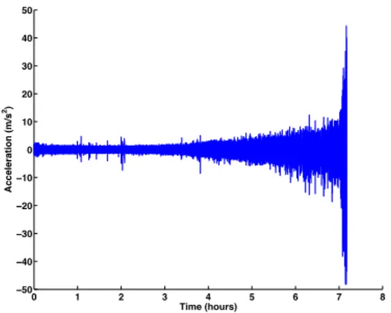
Gathered signals from machine components contain generally immense number of data which require a large amount of memory and computation power to be analysed as shown in Figure 3. In order to transform raw input data into
! " # $ % & ' ( ) −&! −%! −$! −#! −"! ! "! #! $! %! &! * + + , -, ./ 01 2 3 456 78 #9 :16,45;2<.89
Fig. 3: Example of raw signal extracted from bearing test bid
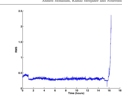
reduced informative representation, different features can be extracted from raw signals. These features can be derived from time domain, frequency domain or joint time-frequency domain. Figure 4 depicts an example of root mean square (RMS) feature extracted from raw signal.
In this work features from both time and frequency domains have been extracted from raw signals and are listed in table 1
0 2 4 6 8 10 12 14 16 18 0 0.5 1 1.5 2 2.5 Time (hours) R MS
Fig. 4: Example of RMS feature extracted from sensory bearing test bid
Table 1: Summary of features extracted from raw signals
Feature Formula
Peak-to-Peak mean(upperpks) + mean(lowerpks)
Maximum peak value max(f indpeaks(signal))
Root mean square q1
n(x 2 1+ x22...+ x2n) Kurtosis E(x−µ) 4 σ4 Skewness N P i=1 (xi−¯x)3 (N −1)σ3
Mutual information I(X, Y ) = H(X) + H(Y ) − H(X, Y )
Entropy H(X) = −P
x∈Xp(x) log p(x)
Arithmetic mean of PSD 20log10
1 n P abs(f f t(x)) 10−5 Line integral i= n P i=0 abs(xi+1− xi) Autoregressive model xt= c + p P i=1 φixt−i+ ǫt Energy e= n P i=0 x2 i
3.2 Unsupervised feature selection
Not all extracted features acquired in the previous step are interesting, that is, contain information about the degradation of the system. We are interested in signals that have non random relationships and consequently contain in-formation about system degradation. To select such signals, an unsupervised feature selection algorithm [24] based on information theory is applied. The algorithm first calculates pairwise symmetrical uncertainty for all the input signals, defined by:
SU(X, Y ) = 2 I(X, Y )
H(X) + H(Y ) (1)
where I(X,Y) is the mutual information between two random variables X and Y ; H(X) and H(Y) are information entropy of a random variable. Then, the algorithm measures the distance between all the pairs using hierarchical clustering. The algorithm finally ranks the resulting clusters according to the quality of the included signals in representing interesting relationships, that is, contain information about machinery degradation using normalised SOM distortion measure. The selected features now can represent the nominal be-haviour of the critical component. Any change in the relations between selected features can indicate a potential fault in the system. The selected features are then compressed into lower dimension using PCA to represent the critical components’ health evolution over the time.
3.3 Features compression
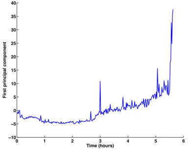
In order to follow the trajectories of selected features over time, the number of features has to be reduced to a compact form. The goal in this step is to compress the n features selected in the previous step onto one-dimensional space. One way to compress the variables, i.e. reducing the number of their dimensions, without much loss of information is by using PCA. PCA projects data from features to principal component domain while keeping the greatest variance by any projection of the data on the first principal component and the second greatest variance on the second principle and so on. PCA can be used for data compression of the input dataset by using one or more of the principle components. In this way, the method can compress the n input features, selected in the previous step, into single trend to represent the health evolution over the time.
In this work we use standard PCA method where eigenvalues λiand
eigen-vectors vihave been calculated for covariance matrix C of the selected features
Then, the first component is used to represent the health status evolution with respect to time as shown in Figure 5. The compressed features are then further processed to get a smooth trend of the health status.
! " # $ % & ' −"! −& ! & "! "& #! #& $! $& %! ()*+,-./0123 4 )1 2 5, 6 1) 7 8 )6 9 :, 8 / * 6 / 7 + 7 5
Fig. 5: Example of group of selected feature compressed using PCA
3.4 Signal trend extraction
So far, the reduced signals exhibit high level of oscillations and noise. Such oscillations make the signal hard for visualisation and superfluous for model building tasks. In this section, the internal structure of the data is extracted in a way which best explains the degradation in a simple monotonic signal and the rest of oscillations are discarded using empirical mode decomposition algorithm (EMD).
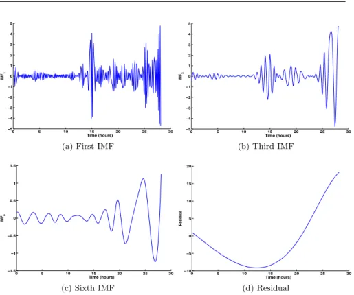
EMD, which was originally proposed by Huang et al [14], is a way for signal decomposition into a successive Intrinsic Mode Functions (IMF), such as depicted in Figure 6, and is composed of the following steps:
– Find all the local maxima and minima of the input signal and compute the
corresponding upper and lower envelopes using cubic spline respectively
– Subtract the mean value of the upper and lower envelopes from the original
signal.
– Repeat until the signal remains nearly unchanged and obtain IM Fi.
– Remove IM Fi from the signal and repeat if it is neither a constant nor a
! " #! #" $! $" %! −" −& −% −$ −# ! # $ % & " '()* (hours) +,-#
(a) First IMF
! " #! #" $! $" %! −" −& −% −$ −# ! # $ % & " '()* (hours) +,-% (b) Third IMF ! " #! #" $! $" %! −#&" −# −!&" ! !&" # #&" '()* (hours) +,-. (c) Sixth IMF ! " #! #" $! $" %! −#! −" ! " #! #" $! &'() (hours) * ) + ', -. / (d) Residual Fig. 6: Example of decomposition process using EMD
3.5 Health Status Modelling
Machine learning provides large methodologies such as simple regression algo-rithms which are used to fit models through training data. In case of regression we assume that the real underlying function is the sum of our estimation and an error, i.e. the error can be estimated by a difference between the real un-derlying function and our estimate:
y= wx + ε ⇒ ε = y − wx (3)
The goal is to use this to find a vector w for which the regression model best fits the training data, which corresponds to finding the minimum value of the error. Usually, this procedure called training the model is done by minimising the sum-of-squares error function for each data point:
E= SSE =
N
X
n=1
There are many linear regression methods which can be used to learn the degradation process. In standard linear regression the pseudo-inverse of the input training data is used to compute the coefficients for a linear model. As the name suggests this involves to invert a matrix and which might not always be possible because of zero eigenvalues of the matrix. Ridge regression tries to cope with this by perturbation of the diagonal entries of the matrix.
If we expand the square in equation 4 and then differentiate the expansion with respect to w we end up with the equation below from where we can isolate w as a function of known data.
XTXw= XTy⇒ w = (XTX)−1XT
y (5)
The major weakness of equation 5 is that the X is a non-square matrix and thus it is not invertible. To solve this problem pseudo-inverse generalisation of the notion of matrix inverse to non-square matrices has been applied.
w= (XT
X)−1XT
y= X†y (6)
Nevertheless, if XTXin equation 6 has zero eigenvalues it is not invertible
and said to be singular. Ridge regression tries to cope with this by adding a
term λI to XTX which perturbs the diagonal entries of XTX to encourage
non-singularity.
XTX⇒ (XTX+ λI) ⇒ w = (XTX+ λI)−1XTy (7)
In a practical application, we need to determine the values of the regression parameter λ, and the principle objective in doing so is usually to achieve the best predictive performance on new data. The performance on the training set is not a good indicator of predictive performance on unseen data due to the problem of over-fitting. Here, we use cross-validation to take the available data and partition it into a training set, used to determine the coefficients w and a validation set used to optimize the model complexity (in this case finding a proper value for λ).
4 Experiments
This work has been verified using two different datasets, PRONOSTIA and NASA datasets. First, the trends have been extracted from the raw data then a selected trend has been modelled for RUL estimation. The details of the datasets and the experiments are explained in the following subsection.
4.1 Trend Extraction 4.1.1 PRONOSTIA dataset
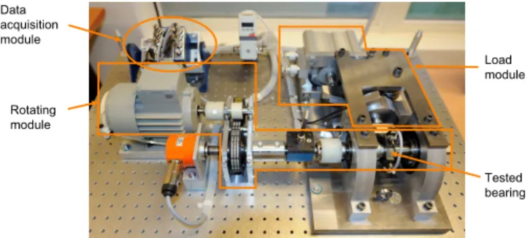
PRONOSTIA, (see Figure 7), is an experimentation platform dedicated to test and validate bearing fault detection, diagnostic and prognostic approaches. It is composed of four main parts: a rotating part, a degradation generation part (with a radial force applied on the tested bearing) a measurement part and test bearings, [26]. In this work three data sets, acquired from this platform, have been used to validate the algorithm, where only the acceleration data has been used. For the first dataset, the algorithm generates 9 signals, each
Tested bearing Data acquisition module Rotating module Load module
Fig. 7: PRONOSTIA experimentation platform
of that represents evolution of the bearing degradation over the time with different trajectories. Figure 8 shows two selected monotonic health indices for the first experiment. As can be seen from the figure the trends show a smooth increasing signals over the time which can be used to deduce health status of the machinery. The plot on the left side is the result of fusing two AR parameters for the first sensor and one parameter for the second sensor. The plot on the right side shows another indicator which was a result of fusing also three features namely, skewness for the first sensor along with the second parameter of AR model and line integral feature extracted from the second sensor signal. Figure 9 shows two selected non-monotonic health indices for the same experiment. The plot on the left side is the result of fusing two fea-tures, skewness of the second sensor and energy of the first sensor. The plot on the right side shows another indicator which was a result of fusing also two features namely, kurtosis and skewness extracted from the second sensor. For the second dataset, the algorithm generates 10 signals, each of that indicates the health degradation over the time. Figure 10 shows two selected monotonic health indices for the first experiment. The plot on the left side; which is al-most linear function, is the result of fusing two features, maximum peak value and AR parameter, both have been extracted from the first sensor. The plot on
0 1 2 3 4 -4 -2 0 2 4 6 8 10 12 14 Time (hours) R e s id u a l (a) ! " # $ % −!&' −!&( −!&% −!&# ! !&# !&% !&( )*+,-./01234 5 ,3*6178 (b) Fig. 8: PRONOSTIA first monotonic dataset
0 1 2 3 4 -4 -2 0 2 4 6 8 Time (hours) Re s id u a l (a) ! " # $ % −"!!! −&!! ! &!! "!!! "&!! '()*+,-./012 3*1(4 /56 (b) Fig. 9: PRONOSTIA first non-monotonic dataset
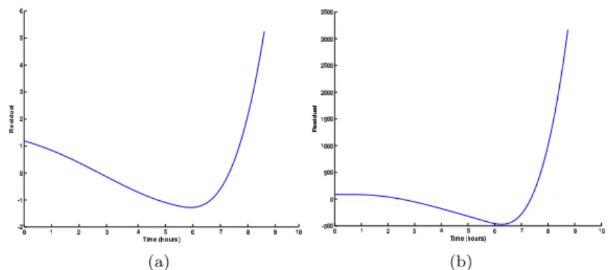
the right side shows a smooth monotonic function. It is a result of fusing also two features, RMS and line integral acquired from the second sensor. Figure 11 shows two selected non-monotonic health indices for the same experiment. The plot on the left side is the result of fusing three features, entropy of both sensors and AR model parameter for the first sensor. The plot on the right side shows another indicator which was a result of fusing four features namely, peak-to-peak, maximum peak value, energy for the second sensor and the mu-tual information between both sensors. For the third dataset, the algorithm generates 9 signals that indicate the health degradation over the time. Figure 12 shows two selected monotonic health indices for the aforementioned experi-ment. The plot on the left side; which is almost linear function, is the result of fusing three features, peak-to-peak, maximum peak value and AR parameter where all the features have been extracted from the first sensor. The plot on the right side shows a smooth decreasing monotonic function. It is a result of fusing three features, arithmetic mean of power spectral density (PSD)
ex-! " # $ % & '! −!(% −!($ −!(# −!(" ! !(" !(# !($ )*+, (hours) -, . */ 0 1 2 (a) ! " # $ % &! −%! −$! −#! −"! ! "! #! $! %! '()* (hours) + *, (-. / 0 (b) Fig. 10: PRONOSTIA second monotonic dataset
(a) ! " # $ % & ' ( ) * −$ −# −" ! " # $ % & +,-./0123456 7 .5, 8 3 9: (b)
Fig. 11: PRONOSTIA second non-monotonic dataset
tracted from both sensors and kurtosis which has been extracted from second sensor.
(a) (b)
Figure 13 shows two selected non-monotonic health indices for the same experiment. The plot on the left side is the result of fusing two features, skew-ness which has been extracted from the first sensor and entropy of the first sensor. The plot on the right side shows another indicator which was a result of fusing two features namely, kurtosis and line integral acquired from second sensor.
(a) (b)
Fig. 13: PRONOSTIA third non-monotonic dataset
4.1.2 NASA dataset
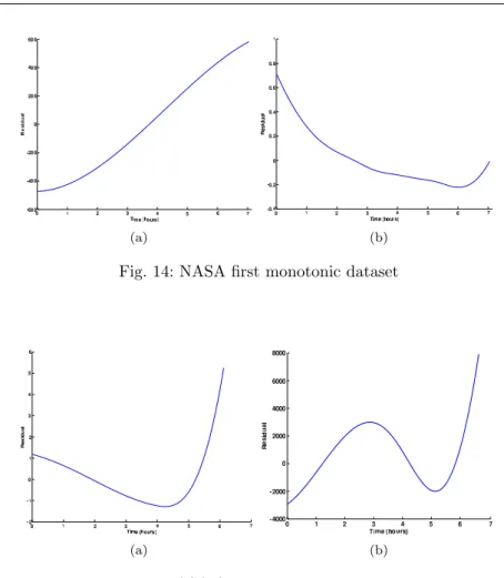
This data set is fully described in NASAs website (ti.arc.nasa.gov/tech/dash/pcoe/). In this work only the first two sensors readings have been used to validate the algorithm. For the first dataset the algorithm generates 10 trends from the raw data. Figure 14 shows two selected monotonic health indices for the afore-mentioned experiment. The plot on the left side shows the result of fusing four features; peak-to-peak, maximum peak value and energy acquired from the second sensor and entropy from the first sensor. The plot on the right side shows a smooth decreasing monotonic function. It is a result of fusing two fea-tures, Mutual information between both sensors and entropy which has been extracted from second sensor. Figure 15 shows two selected non-monotonic health indices for the same experiment. The plot on the left side is the result of fusing two features, maximum peak value which has been extracted from the first sensor and Skewness which has been extracted from the second sensor. The plot on the right side shows another indicator which was a result of fus-ing two features namely, kurtosis and line integral acquired from first sensor. For the second dataset the algorithm generates 6 trends from the raw data. Figure 16 shows two selected monotonic health indices for the aforementioned experiment. The plot on the left side shows the result of fusing two features; maximum peak value acquired from the second sensor and energy acquired from the first sensor. The plot on the right side shows a smooth decreasing
(a) (b) Fig. 14: NASA first monotonic dataset
(a) (b)
Fig. 15: NASA first non-monotonic dataset
monotonic function. It is a result of fusing two features, Entropy of the first sensor and arithmetic mean of PSD acquired from the second sensor. Figure 17 shows two selected non-monotonic health indices for the same experiment. The plot on the left side is the result of fusing two features, peak-to-peak and energy which have been extracted from the second sensor. The plot on the right side shows another indicator which was a result of fusing two features namely, peak-to-peak and entropy acquired from first sensor. For the final dataset the algorithm generates 10 trends from the raw data and non of them was monotonic. Figure 18 shows two selected non-monotonic health indices for the same experiment. The plot on the left side is the result of fusing two features, peak-to-peak; acquired from first sensor, and entropy of both sen-sors. The plot on the right side shows another indicator which was a result of fusing two features namely, root mean square and AR coefficient acquired from second sensor.
! " # $ % &! −%! −$! −#! −"! ! "! #! $! %! '()* (hours) + * , (-. / 0 (a) ! " # $ % & '! −!(% −!($ −!(# −!(" ! !(" !(# !($ )*+, (hours) -,. */0 12 (b) Fig. 16: NASA second monotonic dataset
(a) (b)
Fig. 17: NASA second non-monotonic dataset
0 1 2 3 4 0.2 0.25 0.3 0.35 0.4 0.45 0.5 Time (hours) R e s id u a l (a) (b)
Fig. 18: NASA third non-monotonic dataset 4.2 Ridge regression
From NASA and PRONOSTIA datasets, two trends have been selected for this step. One trend is used for building the regression and the other trend is used
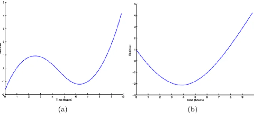
for testing. The experiments have been done on the same time t. Figure 19a and 19b show the original trends for PRONOSTIA and NASA respectively.
! " # $ % −# ! # % & ' "! Time (hours) R esi dual
(a) Training PRONOSTIA dataset
! " # $ % & ' ( ) * −$ −# −" ! " # $ % & +,-./0123456 7 .5, 8 3 9:
(b) Training NASA dataset Fig. 19: Selected trends for modeling
We first calculate the coefficients with minimum error as shown in the pre-vious section. Figures 20a and 20b show the effect of using regression parame-ter λ where the minimum error has been selected for the regression modelling for both PRONOSTIA and NASA respectively. Finally, we test the model by
0 1 2 3 4 5 6 76 77 78 79 80 81 82 Lambda R MS Error validation performance trainning performance lambda for W*
(a) Error minimisation for PRONOS-TIA dataset 0 5 10 15 20 25 30 0 50 100 150 200 250 300 Lambda R MS Erro r validation performance trainning performance lambda for W*
(b) Error minimisation for NASA dataset
Fig. 20: Error minimisation
using test trends for both datasets and calculate the mean absolute error (8).
mean(abs(Expected − Real)) (8)
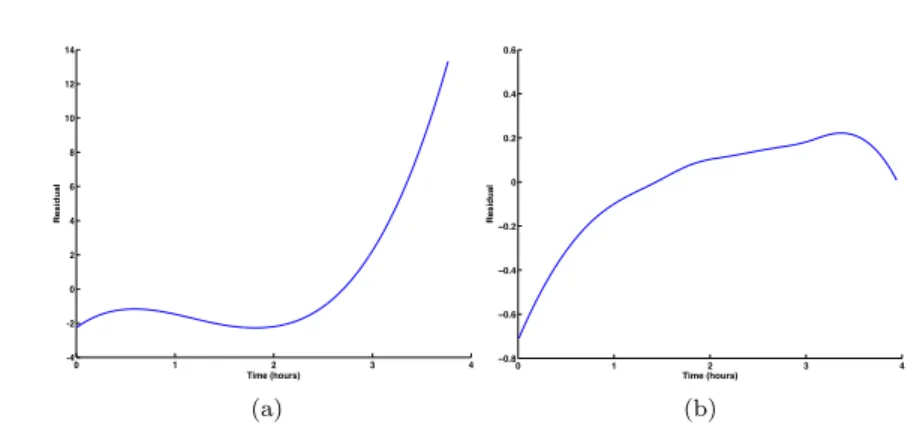
Figure 21a shows the results of predicted trends. The results show that the estimation was so close to the test values with absolute error = 0.4165. Figure
0 1 2 3 4 0 2 4 6 8 10 Time (hours) Resi dual Original Fit
(a) PRONOSTIA dataset expected vs. Real values for first dataset
Fig. 21: Prediction error for PRONOSTIA dataset
! " # $ % & ' ( ) * −# −" ! " # $ % +,-./0123456 7 .5, 839: ;4,<,=9: >,?
(a) NASA dataset expected vs. Real values for first dataset
Fig. 22: Prediction error curves for NASA dataset
22a shows the results of predicted trends. The results show that the estimation was so close to the test values with absolute error = 0.0751.
5 Conclusion
In this work a health estimation model based on unsupervised trend extrac-tion algorithm from sensory data has been proposed. The generated trends showed a smooth representation of the progression of machinery health status and have been used for health degradation modelling. The proposed method is based on extracting successive multi-dimensional features from machinery sensory signals acquired from machines’ critical components. Then, unsuper-vised feature selection on the features domain is applied without making any assumptions concerning the source of the signals and the number of the ex-tracted features. An empirical mode decomposition algorithm (EMD) is ap-plied on the projected features with the purpose of following the evolution of data in a compact representation over time. Finally, a ridge regression has been
applied for the generated trends for modelling the degradation. These models can be used to identify the current machinery health status and predict the RUL of the machine. The algorithm is demonstrated on accelerated degrada-tion dataset of bearings acquired from PRONOSTIA experimental platform and NASA dataset where it is shown to be able to extract interesting signal trends. The results show that the algorithm is generic and can extract the progression of the machinery health status in a compact form. The generated trends have been used also for model building and validation.
References
1. Agogino, A., Tumer, K.: Entropy based anomaly detection applied to space shuttle main engines. IEEE Aerospace Conference (2006)
2. Brown, D., Georgoulas, G., Chen, R., Ho, Y.H., Tannenbaum, G., Schroeder, J.: Particle filter based anomaly detection for aircraft actuator system. IEEE Aerospace conference, Monatan, USA (2009)
3. Camci, F., Medjaher, K., Zerhouni, N., Nectoux, P.: Feature evaluation for effective bear-ing prognostics. Article first published online: 16 MAR 2012 (2012). doi: 10.1002/qre.1396 4. CEMPEL, C.: Multidimensional condition monitoring of mechanical systems in
opera-tion. Mechanical Systems and Signal Processing pp. 1291–1303 (2003)
5. CEMPEL, C.: Multifault condition monitoring of mechanical systems in operation. IMEKO XVII, Croatia pp. 1–4 (2003)
6. Charbonnier, S., Garcia-Beltan, C., Cadet, C., Gentil, S.: Trends extraction and analysis for complex system monitoring and decision support. Engineering Applications of Artificial Intelligence pp. 21–36 (2005)
7. Cottrell, M., Gaubert, P., Eloy, C., Franscois, D., Hallaux, G., Lacaille, J., Verleysen, M.: Fault prediction in aircraft engines using self-organizing maps. Advances in Self-Organizing Maps pp. 37–44 (2009)
8. Filev, D.P., Tseng, F.: Novelty detection based machine health prognostics. International Symposium on Evolving Fuzzy Systems pp. 193–199 (2006)
9. Geramifard, O., Xu, J.X., Pang, C.K., Zhou, J.H., Li, X.: Data-driven approaches in health condition monitoring; a comparative study. 8th IEEE International Conference on Control and Automation pp. 1618–1622 (2010)
10. Geramifard, O., Xu, J.X., Zhou, J.H., Li., X.: Continuous health assessment using a sin-gle hidden markov model. 11th International Conference on Control Automation Robotics and Vision pp. 1347–1352 (2010)
11. Geramifard, O., Xu, J.X., Zhou, J.H., Li, X.: Continuous health condition monitoring: A single hidden semi-markov model approach. IEEE Conference on Prognostics and Health Management pp. 1–10 (2011)
12. Heng, A., Zhang, S., Tan, A.C.C., Mathew, J.: Rotating machinery prognostics: State of the art, challenges and opportunities. Mechanical Systems and Signal Processing pp. 724–739 (2009)
13. Heng, R., Nor, M.: Statistical analysis of sound and vibration signals for monitoring rolling element bearing condition. Applied Acoustics pp. 211–226 (1998)
14. Huang, N.E., Shen, Z., Long, S.R., Wu, M.C., Shih, H.H., Zheng, Q., Yen, N.C., Tung, C.C., Liu, H.H.: The empirical mode decomposition and the hilbert spectrum for nonlinear and non-stationary time series analysis. Proceedings of the Royal Society of London Series A: Mathematical, Physical and Engineering Sciences pp. 903–995 (1998)
15. ISO: Condition monitoring and diagnostics of machines - prognostics - part 1: General guidelines. int. standard ISO 13381-1 (2004)
16. Jardine, A.K.S., Lin, D., Banjevic, D.: A review on machinery diagnostics and prognos-tics implementing condition-based maintenance. Mechanical Systems and Signal Process-ing pp. 1483–1510 (2006)
17. Jiang, H., Penman, J.: Using kohonen feature maps to monitor the condition of syn-chronous generators. Workshop on Neural Network Applications and Tools pp. 89–94 (1993)
18. Jie, S., Hong, G.S., Rahman, M., Wong, Y.S.: Feature extraction and selection in tool condition monitoring system. Advances in Artificial Intelligence pp. 487–497 (2002) 19. Jolliffe, I.T.: Principal Component Analysis and Factor Analysis, chap. chapter 7, pp.
150–166. Principal Component Analysis, Springer Series in Statistics (2002)
20. Kothamasu, R., Huang, S.H., VerDuin, W.H.: System health monitoring and prognos-tics: A review of current paradigms and practices. International Journal of Advanced Manufacturing Technology pp. 1012–1024 (2006)
21. Li, R., Sopon, P., He, D.: Fault features extraction for bearing prognostics. Journal of Intelligent Manufacturing pp. 313–321 (2012)
22. Medjaher, K., Tobon-Mejia, D., Zerhouni, N.: Remaining useful life estimation of critical components with application to bearings. IEEE Transactions on Reliability pp. 292–302 (2012)
23. Miao, Q., Wang, D., , Pecht, M.: A probabilistic description scheme for rotating ma-chinery health evaluation. Journal of Mechanical Science and Technology pp. 2421–2430 (2010)
24. Mosallam, A., Byttner, S., Svensson, M., T., R.: Nonlinear relation mining for maintenance prediction. IEEE Aerospace Conference pp. 1–9 (2011). doi: 10.1109/AERO.2011.5747581
25. Moshou, D., Kateris, D., Sawalhi, N., Loutridis, S., Gravalos, I.: Fault severity estima-tion in rotating mechanical systems using feature based fusion and self-organizing maps. Artificial Neural Networks pp. 410–413 (2010)
26. Nectoux, P., Gouriveau, R., Medjaher, K., Ramasso, E., Chebel-Morello, B., Zerhouni, N., Varnier, C.: Pronostia: An experimental platform for bearings accelerated degradation tests. IEEE International Conference on Prognostics and Health Management, PHM’12, Denver, Colorado, USA (2012)
27. Ocak, H., Loparo, K.A., Discenzo, F.M.: Online tracking of bearing wear using wavelet packet decomposition and probabilistic modeling: A method for bearing prognostics. Jour-nal of Sound and Vibration pp. 951–961 (2007)
28. Pontoppidan, N.H., Larsen, J.: Unsupervised condition change detection in large diesel engines. IEEE 13th Workshop on Neural Networks for Signal Processing pp. 565–574 (2003)
29. Saha, B., Goebel, K., Poll, S., Christophersen, J.: Prognostics methods for battery health monitoring using a bayesian framework. IEEE Transactions on Instrumentation and Measurement pp. 291–296 (2009)
30. Saha, B., Goebel, K., Poll, S., Christopherson, J.: A bayesian framework for remaining useful life estimation. Proc. Fall AAAI Symposium: AI for Prognostics, Arlington, VA (2007)
31. Schwabacher, M.: A survey of data-driven prognostics. AIAA InfoTech Aerospace (2005) 32. Svensson, M., Rognvaldsson, T., Byttner, S., West, M., Andersson, B.: Unsupervised deviation detection by gmm; a simulation study. IEEE International Symposium on Di-agnostics for Electric Machines, Power Electronics and Drives pp. 51–54 (2011)
33. Tavares, G., Zsigraiova, Z., Semiao, V., da Graca Carvalho, M.: Monitoring, fault detec-tion and operadetec-tion predicdetec-tion of msw incinerators using multivariate statistical methods. Waste Management pp. 1635–1644 (2011)
34. Tobon-Mejia, D., Medjaher, K., Zerhouni, N., Tripot, G.: A data-driven failure prog-nostics method based on mixture of gaussians hidden markov models. IEEE Transactions on Reliability pp. 491–503 (2012)
35. Wald, R., Khoshgoftaar, T.M., Sloan, J.C.: Using feature selection to determine optimal depth for wavelet packet decomposition of vibration signals for ocean system reliability. IEEE 13th International Symposium on High-Assurance Systems Engineering pp. 236–243 (2011)
36. Y. Peng, M.D., Zuo, M.: Current status of machine prognostics in condition-based main-tenance: a review. The International Journal of Advanced Manufacturing Technology p. 2010 (297–313)
37. Yang, Z., Zhong, J., Wong, S.F.: Machine learning method with compensation distance technique for gear fault detection. 9th World Congress on Intelligent Control and Au-tomation pp. 632–637 (2011)
38. Zhang, S.: Function estimation for multiple indices trend analysis using self-organizing mapping. IEEE Symposium on Emerging Technologies and Factory Automation pp. 160– 165 (1994)
39. Zhang, S., Hodkiewicz, M., Ma, L., Mathew, J., Kennedy, J., Tan, A., Anderson, D.: Ma-chinery condition prognosis using multivariate analysis. Engineering Asset Management pp. 847–854 (2006)
40. Zhang, X., Xu, R., Kwan, C., Liang, S., Xie, Q., Haynes, L.: An integrated approach to bearing fault diagnostics and prognostics. Proceedings of the 2005 American Control Conference pp. 2750–2755 (2005)
41. Zhou, J.H., Pang, C.K., Lewis, F.L., Zhong, Z.W.: Intelligent diagnosis and progno-sis of tool wear using dominant feature identification. IEEE Transactions on Industrial Informatics pp. 454–464 (2009)