Relieving Flow Limits in Continuation Power
Flows by Generation Rescheduling
Glavic M., Bhat
S., Vassena S.
Abstract— This paper explores an idea to handle flow limits, by means of generation rescheduling before reaching system hard limits, by extension and reformulation of continuation power flow problem. In particular, we focus on the reformulation and extension of a “standard” continuation power flow method so that include generator rescheduling when a flow on a given line exceeds some specified limit, and provide details on analytical expressions to determine most effective generators to be assigned for the limit handling. Four options for active generation rescheduling are considered: based on topology analysis, sensitivity studies, generator margins, and cost considerations. Results of the tests obtained using the IEEE-39 and IEEE-118 bus systems are given to illustrate the performance of the methodology. We also discuss possible extensions of the approach.
Key words: Continuation power flows, generation rescheduling, line flow limits, sensitivity.
I. INTRODUCTION
The continuation power flow (CPF) is one of the most powerful tools employed for maximum loadability determination and voltage stability analysis [1], [3-6]. This methodology enables one to determine the system load margin [1], [4], [7-8], the critical bus [3], [5], and control actions to avoid voltage instability problem [2], [7]. The computational time associated with a continuation power flow may be a barrier, but the accurate results obtained render this methodology as a benchmark for other methodologies.
This paper focuses on soft system limits (we define these as limits that, once reached, can be tolerated or regulated by some action), particularly line flow limits, and gives to a CPF an additional special feature: handling the line flow limits. The system model is based on an efficient variant of CPF termed as “maximum loadability” or Point of Collapse Power Flow, a sparse vectorized, Matlab implementation of a Newton power flow. At the heart of the model is an extremely efficient method for the construction of the Jacobian matrix and complete vectorization of all operations [9-10]. The program has been extended to take into consideration the possibility that limits may be “extended” (up to the point where hard system limit is reached (these are limits that cannot be overcome by any of the acceptable corrective actions), if one is willing to rescheduling generators.
Mevludin Glavic is with the University of Liege, Electrical Engineering and Computer Science Department, 4000 Liege, BELGIUM, (e-mail: [email protected]).
Sunil Bhat is with the Electrical Department, Visvesvaraya National Institute of Technology, Nagpur, India (e-mail: [email protected]). Stefano Vassena is with AREVA T&D, Massy, FRANCE, (e-mail: [email protected]).
Controlling and removing flow limits is not trivial, and the inclusion of a general methodology for flow limits control during the continuation process has not been adequately addressed in the literature. This work considers the prevention of exceeding flow limits through rescheduling of a pair of properly chosen generators.
II. CONTINUATION POWER FLOWS
A CPF employs a continuation method to find the solution path of a set of power flow equations. Effective continuation method, and consequently CPF, solves the problem via four basic elements [1], [4-5]:
• Predictor. Its purpose is to find an approximation for the next solution. Usually tangent [5] or first-order polynomial [4] predictor is employed.
• Parameterization. Mathematical way of identifying each solution on the solution curve. Parameterization augments the system of power flow equations.
• Corrector. Usually, application of Newton method to the augmented system of equations.
• Step length control. Can be done by optimal fixed step length or by adaptive step length control. Power flow equations have to be reformulated to include a continuation (varying) parameter. It is desirable that this parameter has physical meaning. Typical natural parameters of interest include the following: the total system demand, the demand at a given bus or within a given area, the amount of power transfer between two areas or between two buses, some other parameters such as the impedance of a line, etc.
The result of these studies is often a set of curves illustrating the behavior of one or more system variables as a function of the parameter. Considering of the demand at a single bus as a varying parameter is not realistic, but can be used to detect weak buses and to express the system robustness. Using of the total system demand or the demand at several buses are more realistic (load increase can be based on the existing load profile or a load forecast). For purpose of this paper we consider the total system demand as varying parameter. Let, an electric power system be modeled by the power flow equations, 0 ) , (x λ = f (1) where x is the vector of state variables (voltage magnitudes and angles at load buses, voltage angles at generator buses) and λ is a vector of parameters. In the continuation power flows the objective is to study how solutions of (1) vary as parameters are changed. If one parameter is varied, then a curve results, if two
IV CONGRESO INTERNACIONAL DE INGENIERIA ELECTROMECANICA Y DE SISTEMAS
del 14 al 18 de noviembre de 2005, México, D.F. ELE-207
parameters are allowed to change then a surface is obtained, variation of more parameters results in a higher dimensional hypersurface. To have an applicable continuation power flow one has to take care about three, among many, very important things: physical meaning of parameter (in this paper total system load demand), load modeling, and generation rescheduling. Load modeling includes the constant power and non-linear load models. Non-linear load model which include a voltage dependency, generally has the form,
β α = = 0 0 0 0 ; V V Q Q V V P P (2)
where, P0 and Q0 are initial active and reactive powers consumed by the load, α and β are voltage dependency coefficients and V0 initial voltage at the bus. In order to use this load model in a continuation power flow, the load parameter and load increase multipliers must be somehow added so that various load changes can be simulated. This can be done as follows,
(
)
i i i Li Li Li V V P k P α λ + = 0 0 1 (3)(
)
i i i Li Li Li V V Q k Q β λ + = 0 0 1 (4)where PLi0 and QLi0 are original loads at bus i, active and reactive respectively, kLi multipliers to designate the rate of load change at bus i. Parameter λ in this formulation corresponds to the quantity of connected load. The load change can be expressed as,
∑
= − = ∆ n i total Li total P P P 1 0 (5) where Ptotal is the total active power load at any given instant and Ptotal0 is the total active power load in the base case. Load increase is compensated by letting each generator (or some of generators) to take up a fraction of the load change. The simplest assumption is to consider that all of generators are adjusted in a predetermined direction (Fixed Dispatch Policy). This direction can be entirely arbitrary, or more likely, chosen in a rational manner (natural choice is that all units under AGC be utilized for load increase compensation, another possibility is rationally chosen load following units). If each generator is made to take up a fraction kGi of the load change, generation at the bus i is given by,total Gi Gi
Gi P k P
P = 0 + ∆ (6)
When the newly formulated load and generation terms are inserted in the general form of power flow equations the result is,
Ti Li n i total Li Gi Gi i P k P P P P P − − − + = ∆
∑
=1 0 0 (7) Ti Li Gi i Q Q Q Q = − − ∆ 0 (8) where the subscript T represent injection. The set of equations that describe the entire system are made up of a combination of these two general equations.The structure of Jacobian matrix associated with the continuation method is given by,
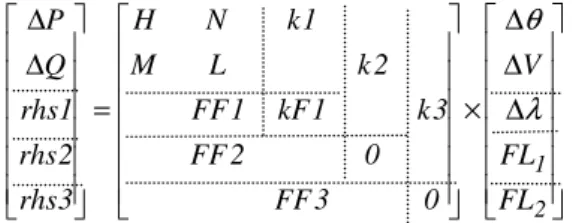
∆ ∆ ∆ × = ∆ ∆ λ θ V 1 kF 1 FF 1 k L M N H rhs Q P (9)
where 1k represents the predetermined generation and load increase direction, FF1 and kF1 correspond to parameterization equation. During “normal” region of continuation, kF1 equals one and FF1 is a zero row. When the ordinary set of equations becomes ill conditioned a different parameterization takes place, λ
becomes a state variable, and an old state variable, e.g., a voltage magnitude of a system bus becomes the system parameter.
III. FLOW LIMITS AND GENERIC FLOW JACOBIAN MATRIX
The factors influencing the limiting values of line flows are: thermal limit (I2f limit, f stands for flow), small-signal stability limit (Pf limit), and voltage difference limit (Sf limit). Flow limits are generally soft and can be relieved by: load reduction, generation rescheduling, and using phase shifters.
Using phase shifters for control purposes is subject of ongoing research. Load reduction as a control action affects all system limits. Voluntary curtailment load by costumer upon notice relieve slow-developing problems which result from changing system conditions. Involuntary load interruption falls in the category of load shedding, and is limited to immanent and severe conditions. The main idea behind the methodology considered in this paper is to handle flow limits, by means of generation rescheduling as the corrective action, before reaching system hard limits. We base our derivation upon generic flow Jacobian matrix to determine most effective generators to handle specific limit.
∂ ∂ ∂ ∂ = V l l Jf f , f θ , (10)
where l denotes generic line flow equation, and f denotes the number of 2 terminal lines in the system. Depending of the limit considered, l becomesI2, P, or S. To calculate the elements of the matrix we introduce the next notation:
f
V - vector of line voltages (Vf = ATV ), f
I - vector of injected current of line (If =YfVf ), f
N
A ×2 - an associate relationship matrix, )
2 2 ( f f f
Y × - the primary admittance matrix in which the diagonal elements are small admittance matrix (2-port representation of branch and transformer),
•- is defined as point-wise multiplication of two vectors.
N denotes the number of buses, and f denotes the number of 2 terminal lines in the system.
The elements of the flow Jacobian matrix are calculated as follows, ) ( jθ T T f e diag A V V A V V = ∂ ∂ = ∂ ∂ (11) ) ( jV diag A V A Vf T T = ∂ ∂ = ∂ ∂ θ θ (12) ) ( jθ T f f f e diag A Y V V Y V I = ∂ ∂ = ∂ ∂ (13) ) ( jV diag A Y V Y I T f f f f = ∂ ∂ = ∂ ∂ θ θ (14) ) ( ) ( )) ( ( T jθ f f e diag A Y conj V I conj − = ∂ ∂ (15) ) ( ) ( )) ( ( jV diag A Y conj I conj T f f − = ∂ ∂ θ (16) θ θ θ ∂ ∂ + ∂ ∂ = ∂ ∂ ( ( )) ) ( )) ( ( 2 f f f f f conj I I diag I I conj diag I (17) V I conj I diag V I I conj diag V I f f f f f ∂ ∂ + ∂ ∂ = ∂ ∂ ( ( )) ) ( )) ( ( 2 (18) ∂ ∂ + ∂ ∂ = = • ∂ ∂ = ∂ ∂ θ θ θ θ )) ( ( ) ( ( ) ( ) ( ) ) ( ) ( ( f f f f f f f f f V conj V conj diag V V diag Y conj V V conj Y conj S (19) ∂ ∂ + ∂ ∂ = = • ∂ ∂ = ∂ ∂ V V conj V conj diag V V V diag Y conj V V conj Y conj V V S f f f f f f f f f )) ( ( ) ( ( ) ( ) ( ) ) ( ) ( ( (20) where: V V ejθ = point wisely.
IV. RELIEVING FLOW LIMITS BY GENERATION
RESCHEDULING
The selection of the rescheduling unit or units can be done in many ways. We specifically consider four ways in which this can be done:
• The user has pre-designated which generators are to be rescheduling, either for all constraints or, better yet, for every possible constraint the user has specified the corresponding pair of generators that are to be rescheduling. We call this type of rescheduling “User (operator) specified”.
• The program is to determine the generator pair using a “most effective” criterion. That is, the generator pair that will have the maximum impact on limiting the flow with the minimum amount of rescheduling is designated as the generator pair of interest. This type of rescheduling is referred to as “Most effective”.
• The program is to determine the generator pair using a “maximum margin” criterion. That is, the generators that are capable of doing the rescheduling with a minimum percentage impact to their available limits are used for the purpose. We call this type of rescheduling “Sufficient”
• The program determines the generator pair based on a minimum rescheduling cost criterions. This type of rescheduling is termed as “Cheapest”. Further we consider two options for the “operator-specified” rescheduling: “Chunk” and “Continuous”. In “Chunk” option the operator simply specifies a generator pair and the amount of active power to be rescheduling. In “Continuous” rescheduling the operator specifies a generator pair, but not the amount of active power to be rescheduling which is to be solved. “Most effective” rescheduling is eminently technical. The choice of a proper generator pair is based on sensitivities of the line flow in relation to each system generator. A proper generator pair for “sufficient” and “cheapest” rescheduling is chosen according to the next formulation,
) (
" "
"
"Sufficient = Most effective× Pmax−Pactual ; ‘INC’,
) (
" "
"
"Sufficient = Most effective× Pactual −Pmin ; ‘DEC’,
$ " "
"
"Cheapest = Sufficient× ; for both, ‘INC’ and ‘DEC’. where “INC” stands for increase and “DEC” for decrease.
A. Finding the most effective generator pair
It is clear from previous subsection that finding the most effective generator pair to handle a limit is in the core of all proposed rescheduling strategies.
To find the most effective generators we rely on flow Jacobian matrix and we first introduce vector FF2 as follows, f T J e FF2= 1 (21) where e1 is the vector with all entries equal to zero but one corresponding to the limited line equal to 1.
The vector of sensitivities of flows to injections for all generators in the system (or at least the eligible subset) can be formulated as,
T T g FF J FF FF s =( 2⋅ 2 )−1 ⋅ 2 (22) The largest-valued entry in sg identifies the system generator where a generator would have the greatest positive impact on the line flow of interest. The smallest-valued entry (most negative) in sg identifies the system generator where a generator would have the greatest adverse impact on the flow.
Let M generators be assigned to participate in flow limit handling. Let introduce a vector 2k containing M nonzero elements. Nonzero value corresponding to i−th ‘INC’ generator is calculated by,
∑
∈ = ' ' 2 INC j j i i FDF FDF k , (23)and for corresponding ‘DEC’ generator,
∑
∈ − = ' ' 2 DEC j j n n FDF FDF k . (24)where FDFsare sensitivities taken from sg.
V. CONTINUATION POWER FLOW WITH FLOW LIMITS AND
GENERATOR RESCHEDULING
Extending the formulation and solutions method of the CPF, so that when the flow on a given line exceeds some specified limit, generation is rescheduling just until the point where the limit is no longer violated, can be done by inclusion of a new row (FF2) and a new column (k2) in the system Jacobian [11], as follows,
∆ ∆ ∆ × = ∆ ∆ FL V 0 2 FF 1 kF 1 FF 2 k L M 1 k N H 2 rhs 1 rhs Q P λ θ (25)
As soon as the limit is identified, the line is kept at the limit by explicit inclusion of this equation. If a second limit is identified, another rescheduling pair is identified and the following Jacobian structure evolves,
∆ ∆ ∆ × = ∆ ∆ 2 1 FL FL V 0 3 FF 0 2 FF 3 k 1 kF 1 FF 2 k L M 1 k N H 3 rhs 2 rhs 1 rhs Q P λ θ (26)
In the structure above,FF3, rhs3, and k3 have the same meaning as FF2, rhs2, and k2. Notice the method provides different values of rescheduling FL1 and FL2, enabling the method to handle a number of different constraints simultaneously. As one can see from (26), including new constraint is straightforward.
VI. RESULTS
The proposed methodology is demonstrated on the IEEE-39 and IEEE-118 bus systems [12]. In the case when the flow limits in all transmission lines are taken to infinity (no flow limits), the system reaches voltage collapse limit, and maximum loadabilities are 11998.54 MW (IEEE-39) and 19250.38 MW (IEEE-118). Two tests were carried out on the IEEE-39 bus system. In the first case the flow limit in line 9 (between buses 4 and 14) is reached at load level 7029.87 MW. “Operator-specified” (continuous) rescheduling option is used to handle the reached flow limit. The chosen generator pair is (‘INC’=35) and (‘DEC’=32). Fig. 1. illustrates the results.
Fig. 1. PV curve of Bus 26 (IEEE-39 bus system)
In the second case, with the same line flow limit reached at the same load level, “Most effective” rescheduling option is used, and results are presented in
the same figure. The proper generator pair is ‘INC’=30, ‘DEC’=32. Fig. 1. shows that in the case of “Most effective” rescheduling option the system can be steered further than in case of “Operator-specified” rescheduling, because this option is eminently technical. In both cases the system meets the voltage collapse limit at the end. “Sufficient” rescheduling option is used in the test carried out on IEEE-118 bus system.
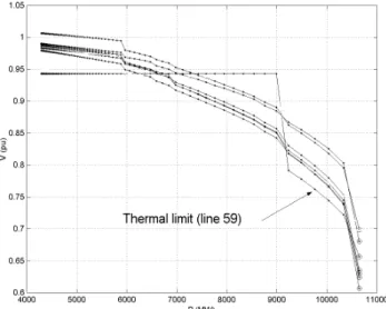
Fig. 2. shows the PV curve associated with the system critical bus at the bifurcation point (bus 95). The flow limit in line 69 (between buses 48 and 49) is reached at the load level 10488.35 MW. The generator pair to act according to “Sufficient” rescheduling is ‘INC’=46, ‘DEC’=49.
Fig. 2. PV curve of Bus 95 for various system conditions At load level 13997.63 MW the system reaches the voltage collapse limit. Two additional tests were carried out on the same test system, one by using “Cheapest” rescheduling option (linear generation costs are considered) with the same assumptions (P and Q generation limits are not considered), and another one with Q generation limits consideration and using “Sufficient” option.
The results are presented in the same figure. For this particular case, the same generator pair has been chosen to handle the reached flow limits. To make a difference from the previous test, the second flow limit (line 71) is reached at load level 11334.21 MW. The process is stalled. If Q generation limits are considered, the flow limit in the same line is reached at load level 8237.73 MW. The same generator pair has been chosen again (“Sufficient” rescheduling option). At load level 8726.30 MW ‘INC’ generator reaches its upper Q limit what results in rapid voltage drop. The next generator picked to increase output is generator 69, eventually the system reaches voltage collapse limit at load level of 9115.18 MW.
One important aspect about this problem must be considered: the “lack” of generators available to handle the flow limits. This happens, basically, because of the next reason: generators electrically close to the limited
line have already reached their P limits, sensitivities calculation indicates, still available, generators most likely to act, but “recommended” generation pair is electrically far away from the flow limited line. To demonstrate capabilities of used point of collapse power flow, with the special features added, another test was carried out with help of IEEE-118 bus system where all limits are considered (see fig. 3.).
Fig. 3. PV curves of some system buses (all limits considered) At the load level amount of 9739.98 MW the thermal limit in transmission line between buses 43 and 44 is identified. Rescheduling option employed is “Operator-specified”. User choice of a proper generator pair is based on the inspection of the system topology, and generator 46 is chosen as the ‘INC’, whereas generator 40 is assigned to ‘DEC’. This is because these generators are the closest ones to ending buses of the limited line. The system reaches voltage stability limit at the load level of 10156.92 MW. The results of the tests carried out are summarized in Table I.
TABLE I
SUMMARY OF THE RESULTS CARRIED OUT ON TWO TEST SYSTEMS Test system Load level at limit MW (1) Maximum loadability MW (2) (1) - (2) Rescheduling option 7029.87 7158.60 128.73 Operator spec. (cont.) IEEE-39 7029.87 7256.34 226.47 Most effective 10488.35 13997.63 3509.28 Sufficient 10488.35 (1st) 11334.21 (2nd) 11351.87 863.52 Cheapest 8237.73 9115.18 877.45 Sufficient IEEE-118 9739.98 10156.92 416.94 Operator spec. (chunk)
In all the tests it has been assumed that load increase direction is pre-specified. In the real world loads vary in a not fully predictable manner. Load variations tend to be correlated to time of day and to weather (particularly temperature). Significant system demand variations tend to be “slow” in time frame of minutes and hours. The methodology is capable to handle changes in load direction and with a reasonable load forecast model incorporated, and with already incorporated sparse matrix and vectorized computing methods, on-line implementation of the methodology will be possible.
VII. DISCUSSION AND FUTURE EXTENSIONS
In deregulated environment, some generation unit owners may not be willing to participate in the generation rescheduling process for their own economic interest [13]. This is the issue to be further investigated in analyzing applicability of the proposed methodology in deregulated environment. We strongly believe that the methodology considered in this paper has potential to be used in deregulated environment since it is based on the idea of implementing a good sub-optimal reschedule involving only a few generation units rather than truly optimal one involving many.
Further work will be focused on extension and formulation of the CPF so that include phase shifters to relieve the flow limits and the methodology application in the design of thermal overload system protection schemes. Moreover, examination of appropriate selection of load following units [14] in CPF to enhance voltage stability and control of power systems in conjunction with the proposed rescheduling scheme might bring more flexibility and the strength to the proposed methodology.
VIII. CONCLUSIONS
Explicit specification of generation rescheduling strategies possible for flow limit handling has been presented in this paper. Sparse vectorized Newton implementation used in the point of collapse power flow has been easily extended. This new feature (together with further inclusion of phase shifters) rendering the tool as a powerful and accurate helper for operating a power system within its security constraints. The operator is allowed to identify the generator pair to be assigned for limit handling according to four different options, based on topology analysis, sensitivity studies, generator margins, or cost considerations. Only thermal line flow limit has been considered in the paper and including other two limits is straightforward. The results carried out with the help of the IEEE-39 and IEEE-118 bus system indicate that the methodology is effective.
REFERENCES
[1] Canizares C. A., Alvarado F. L., ”Point of Collapse and continuation methods for large ac/dc systems, ”IEEE
Trans. Power Systems, vol. 8, no. 1, 1993, pp. 1-8.
[2] Dobson I., Lu L., “Computing an Optimal Direction in Control Space to Avoid Saddle Node Bifurcation and Voltage Collapse in Electric Power Systems”, IEEE Trans.
Automatic Control, Vol. 37, No. 10, 1992, pp. 1616-1620.
[3] Chiang H. D., Flueck A., Shah K. S., Balu N., “CPFLOW: A Practical Tool for Tracing Power System Steady State Stationary Behavior due to Load and Generator Variations”,
IEEE Trans. Power Systems, Vol. 10, No. 2, 1995, pp.
623-634.
[4] Glavic M., “The Continuation Power Flow: A tool for Parametric Voltage Stability and Security Analysis”, Proc.
of 59th American Power Conference APC’97, Chicago,
1997, pp. 1298-1304.
[5] Zambroni de Souza A. C., Cañizares C. A., Quintana V. H., ”New Techniques to Speed up Voltage Collapse Computations Using Tangent Vectors”, IEEE Transactions
on Power Systems, Vol. 12, No. 3, 1997, pp. 1380-1387.
[6] Greene S., Dobson I., Alvarado F. L., “Contingency Analysis for Voltage Collapse via Sensitivities from a Single Nose Curve”, IEEE Trans. Power Systems, Vol. 14, No. 1, pp. 232-240, 1999.
[7] Van Cutsem T., Vournas C., “Voltage Stability of Electric
Power Systems”, Kluwer Academic Publisher, Boston,
1998.
[8] Greene S., Dobson I., Alvarado F. L., “Sensitivity of Transfer Capability Margins with Fast Formula”, IEEE
Trans. on Power Systems, Vol. 17, No.1 1, 2002, pp.34-40.
[9] Alvarado F. L., “Solving Power Flow Problems with a Matlab Implementation of the Power System Applications Data Dictionary”, Proc. of HICSS-32, Maui, Hawaii, June 1999, [Online], Available: http://www.pserc.wisc.edu [10] Mahseredijan J., Alvarado F., Rogers G., Lon W.,
“MATLAB’s Power for Power Systems”, IEEE Computer
Applications in Power, pp. 13-19, 2001
[11] Dobson I., Greene S., Rajaraman R., DeMarco C., Alvarado F., Glavic M., Zhang, J., Zimmerman R., ”Electric Power Transfer Capability: Concepts, Applications, Sensitivity, Uncertainty”, PSERC Report
01-34, ECE Department, University of Wisconsin, Madison, USA, 2001.
[12] “Power System Test Case Archive”, [Online], Available: http://www.ee.washington.edu/research/pstca/
[13] Talukdar B. K., Sinha A. K., Mukopadhyay S., Bose A., ”A computationally simple method for cost-efficient generation rescheduling and load shedding for congestion management”, Electric Power and Energy Systems, vol. 27, 2005, pp. 379-388.
[14] Zecevic A. I., Miljkovic D. M., ”Enhancement of voltage stability by an optimal selection of load following units”, Electric Power and Energy Systems, vol. 23, 2001, pp. 443-450.