Advances in scaling deep learning algorithms

(1)

Universit´e de Montr´eal

par Yann N. Dauphin

Département d’informatique et de recherche opérationnelle Faculté des arts et des sciences

Thèse présentée à la Faculté des arts et des sciences en vue de l’obtention du grade de Philosophiæ Doctor (Ph.D.)

en informatique

June, 2015

c

(2)

Résumé

Les algorithmes d’apprentissage profond forment un nouvel ensemble de m´ e-thodes puissantes pour l’apprentissage automatique. L’idée est de combiner des couches de facteurs latents en hierarchies. Cela requiert souvent un coût compu-tationel plus elevé et augmente aussi le nombre de paramètres du modèle. Ainsi, l’utilisation de ces méthodes sur des problèmes à plus grande échelle demande de réduire leur coût et aussi d’améliorer leur régularisation et leur optimization. Cette thèse adresse cette question sur ces trois perspectives.

Nous étudions tout d’abord le problème de réduire le coût de certains algo-rithmes profonds. Nous proposons deux méthodes pour entrainer des machines de Boltzmann restreintes et des auto-encodeurs débruitants sur des distributions sparses à haute dimension. Ceci est important pour l’application de ces algorithmes pour le traitement de langues naturelles. Ces deux méthodes (Dauphin et al.,2011;

Dauphin and Bengio, 2013) utilisent l’échantillonage par importance pour ´ echan-tilloner l’objectif de ces modèles. Nous observons que cela réduit significativement le temps d’entrainement. L’accéleration atteint 2 ordres de magnitude sur plusieurs bancs d’essai.

Deuxièmement, nous introduisont un puissant régularisateur pour les méthodes profondes. Les résultats expérimentaux démontrent qu’un bon régularisateur est crucial pour obtenir de bonnes performances avec des gros réseaux (Hinton et al.,

2012). Dans Rifai et al. (2011), nous proposons un nouveau r´egularisateur qui combine l’apprentissage non-supervis´e et la propagation de tangente (Simard et al.,

1992). Cette méthode exploite des principes géometriques et permit au moment de la publication d’atteindre des résultats à l’état de l’art.

Finalement, nous consid´erons le probl`eme d’optimiser des surfaces non-convexes `

a haute dimensionalité comme celle des réseaux de neurones. Tradionellement, l’abondance de minimum locaux était considéré comme la principale difficulté dans ces problèmes. Dans Dauphin et al. (2014a) nous argumentons à partir de r´ esul-tats en statistique physique, de la théorie des matrices aléatoires, de la théorie des réseaux de neurones et à partir de résultats expérimentaux qu’une difficulté plus profonde provient de la prolifération de points-selle. Dans ce papier nous proposons aussi une nouvelle méthode pour l’optimisation non-convexe.

Keywords: apprentissage profond, r´eseaux de neurones, optimisation `a haute dimensoin, machine de Boltzmann, auto-encodeurs.

(3)

Summary

Deep learning algorithms are a new set of powerful methods for machine learn-ing. The general idea is to combine layers of latent factors into hierarchies. This usually leads to a higher computational cost and having more parameters to tune. Thus scaling to larger problems will require not only reducing their computational cost but also improving regularization and optimization. This thesis investigates scaling from these three perspectives.

We first study the problem of reducing the computational cost of some deep learning algorithms. We propose methods to scale restricted Boltzmann machines (RBM) and denoising auto-encoders (DAE) to very high-dimensional sparse dis-tributions. This is important for applications of deep learning to natural language processing. Both methods (Dauphin et al., 2011; Dauphin and Bengio, 2013) rely on importance sampling to subsample the learning objective of these models. We show that this greatly reduces the training time, leading to 2 orders of magnitude speed ups on several benchmark datasets without losses in the quality of the model. Second, we introduce a powerful regularization method for deep neural nets. Experiments have shown that proper regularization is in many cases crucial to obtaining good performance out of larger networks (Hinton et al., 2012). In Rifai et al.(2011), we propose a new regularizer that combines unsupervised learning and tangent propagation (Simard et al.,1992). The method exploits several geometrical insights and was able at the time of publication to reach state-of-the-art results on competitive benchmarks.

Finally, we consider the problem of optimizing over high-dimensional non-convex loss surfaces like those found in deep neural nets. Traditionally, the main difficulty in these problems is considered to be the abundance of local minima. In

Dauphin et al. (2014a) we argue, based on results from statistical physics, random matrix theory, neural network theory, and empirical evidence, that the vast major-ity of critical points are saddle points, not local minima. We also propose a new optimization method for non-convex optimization.

Keywords: deep learning, neural networks, high-dimensional non-convex opti-mization, Boltzmann machines, auto-encoders.

(4)

List of Figures

2.1 Graphical depiction of a one layer neural network (DNN) . . . 12

2.2 Graphical model of the restricted Boltzmann machine (RBM) . . . 15

2.3 Schematic of the Denoising Auto-Encoder . . . 21

2.4 Graphical model of the deep belief network (DBN). Image repro-duced from Bengio (2009b). . . 26

4.1 Schematic of the Denoising Auto-Encoder . . . 35

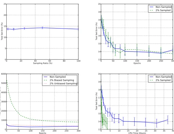
4.2 Experimental Results of reconstruction sampling on Amazon (small set) . . . 43

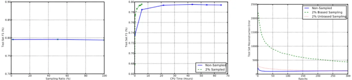
4.3 Experimental Results of reconstruction sampling on RCV1 . . . 44

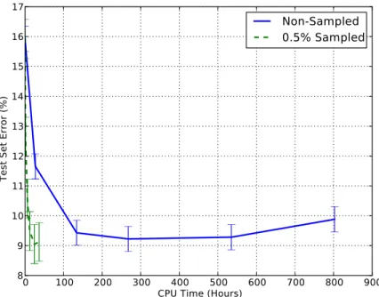
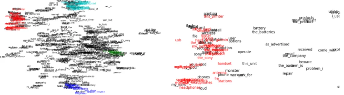
4.4 Learning curve with reconstruction sampling on the Full Amazon set 46 4.5 Embedding learned by the sampled DAE on Amazon . . . 46

6.1 Average speed-ups achieved with SRM . . . 58

6.2 Average norm of the gradients for xi = 1 and xi = 0 . . . 59

8.1 Visualization of the tangents learned by CAEs . . . 75

8.2 Visualization of the tangents learned by local PCA . . . 75

10.1 Empirical validation of the prevalence of saddle points . . . 84

10.2 Behavior of optimizers near saddle points . . . 86

10.3 Evaluation of optimization methods for small MLPs . . . 90

10.4 Empirical results using SFN for deep auto-encoders and recurrent networks . . . 93

(9)

List of Tables

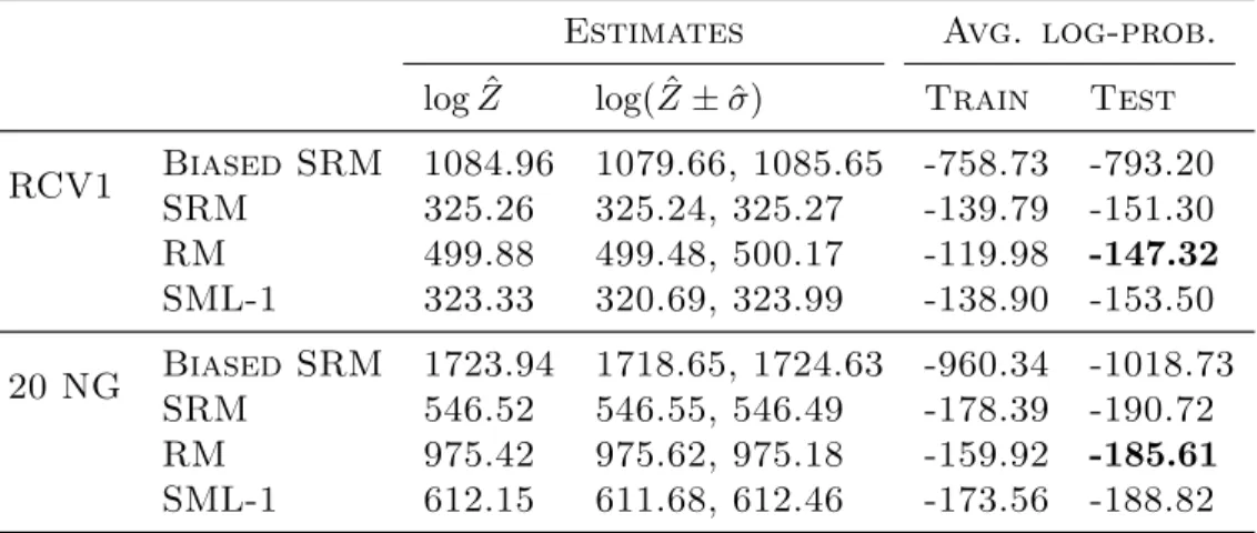
6.1 Generative performance of the RBMs trained with SRM. . . 57

6.2 Classification results on RCV1 for SRM pretrained DNNs . . . 59

6.3 Classification results on 20 Newgroups for SRM pretrained DNNs . 60

8.1 Classification accuracy with the tangent distance given by the CAE 76

8.2 Classification results with the MTC in a semi-supervised setting . . 76

8.3 Classification results with the MTC in a fully supervised setting . . 77

(10)

List of Abbreviations

AE Auto-Encoder

AIS Annealed Importance Sampling CAE Contractive Auto-Encoder

CD Contrastive Divergence

CNN Convolutional Neural Network DAE Denoising Auto-Encoder DBN Deep Belief Network DNN Deep Neural Network

I.I.D Independent and Identically-Distributed KL Kullback-Leibler

MLP Multi-Layer Perceptron MTC Manifold Tangent Classifier

PCD Persistent Contrastive Divergence

RBM Restricted Boltzmann Machine RM Ratio Matching

SDAE Stacked Denoising Auto-Encoder SFN Saddle-Free Newton

SGD Stochastic Gradient Descent SML Stochastic Maximum Likelihood SRM Stochastic Ratio Matching SVM Support Vector Machine

(11)

Acknowledgments

I feel lucky to have been part of the LISA lab (predecessor of the MILA). Yoshua Bengio instilled in his lab a deep passion for creativity and a degree of openness that allows collaboration to flourish. This has had a profound impact on me. I am also grateful to Yoshua for the experience and advice he has shared with me.

I am thankful to have had amazing people to discuss and argue about ideas with. There have been too many to count, but I am particularly in the debt of my collaborators: Salah Rifai (AKA the idea factory), Xavier Glorot, Gregoire Mesnil, Xavier Muller, Harm de Vries, Pascal Vincent, Surya Ganguli, Kyun-hyun Cho, Caglar Gulcere. I would also like to thank Ian Goodfellow, Aaron Courville, Guillaume Alain, Laurent Dinh and Mehdi Mirza. Frederic Bastien too for his work on Theano and giving us clusters that work. These are some of the people that have made my days at the lab pleasant.

I am also thankful to my parents for sharing with me their passion for knowledge and my aunts, cousins and friends for supporting me through these 5 years. To my roommates Fedo, Manu and Marina sorry for forgetting the milk so many times but it was for a good cause. And thanks to Robert Panet-Raymond for taking the time to do a college course that motivated me to do a Ph.D.

(12)

1

Introduction

Deep learning algorithms are a new development in machine learning. They are generating a lot of interest because they have achieved state-of-the-art results in significant benchmarks for artificial intelligence. These tasks include computer vision (Krizhevsky et al., 2012), language modelling (Mikolov et al., 2011), and automatic speech recognition (Seide et al., 2011). These advances and theoreti-cal considerations have led some to hypothesize that deep learning may be a key component in learning AI-hard tasks (Bengio, 2009a). AI-hard tasks are those whose difficulty is equivalent to solving general purpose artificial intelligence. In particular, deep learning is a powerful solution to the problem of perception in intelligent systems. Whereas traditional machine learning requires humans to craft task-specific features, deep learning automatically learns features from raw data. It does so by learning a hierarchy of non-linear features from the input data. One significant challenge that remains to be solved on the road to solving AI-hard tasks is that of scale. Deep learning algorithms must be scaled both in terms of the sizes of the datasets they can handle and the size of the models themselves. For reference, one of the biggest deep learning (Krizhevsky et al.,2012) system has 109

connections, while the human brain has 1015 _{connections. This thesis studies the}

issue of scaling deep learning algorithms.

Chapter 1 is an introduction to machine learning. It is followed by a review of the new developments brought forth by deep learning in Chapter 2. The sub-sequent chapters describe work that has been done in the context of this thesis. Chapters 4 and 6 describe new methods to scale unsupervised deep learning algo-rithms to high-dimensional sparse distributions. In chapter 8, we propose a new regularization method for large deep neural networks. Finally, we investigate the problem of optimizing high-dimensional deep neural networks in chapter 10 and propose practical solutions.

(13)

1.1 Introduction to machine learning

Machine learning is the study of algorithms that can learn from examples. It is a form of artificial intelligence that combines notions from both statistics and optimization. The goal of a learning algorithm is to automatically learn a function

ˆ

f that can perform some task of interest. In comparison, most other AI approaches

rely on human labor to specify program behaviour (Hayes-Roth et al., 1984). The distinctive quality of learning algorithms is that they are not explicitly programmed for the task of interest. For example, such an algorithm could learn to differentiate between cats and dogs using only a set of examples D = {(x0, y0), . . . , (xn, yn)}.

On the one hand, the algorithm must discover the hidden statistical link between the images xi and the corresponding labels yi. This involves a search process over

many different functions or hypotheses. Based on the dataset D it might reach the hypothesis for instance that cats have upright ears while dogs do not. However, it is not as simple as finding an hypothesis that fits the dataset. While all the dogs in D may have droopy ears it does not guarantee that all dogs do. Machine learning requires statistical induction: how to make good inferences from past data. Thus, the learning algorithm must find a hypothesis that fits the available data and even the unseen future data. This section explains how machine learning solves this problem.

In machine learning, learning consists in searching for the best function f within a family of functions F that performs a task. This function f is found through optimization. The ability of a function f to perform the task is measured by a so-called loss function L. For example, the error function might measure the number of misclassified objects within D. Mathematically, we can express learning as approximating the following operation

ˆ f = arg min f ∈F 1 |D| X (x,y)∈D L(f (x), y) (1.1)

In other words, we are trying to find a function ˆf that most accurately predicts

the labels y from the inputs x. While there are other formulations, this one reveals some of the key aspects of machine learning. First, it is key to find an efficient approximation of the arg min operation. The naive solution of exhaustive search on the set F will not scale. There are several models families where F is infinite.

(14)

In practice, optimization methods are used to navigate the space. We will discuss some of these methods in Section 1.3. Another important aspect is the choice of the model family F . There are many different families like neural networks and support vector machines. We will cover several in Section 1.2. The choice of the model family will influence the ease of optimizing the model. More importantly, it determines how well we will be able to mimic the true function f∗(x) = y with

ˆ

f . If the model family is too small, it may not include a function that matches f∗. This can be one of the causes of underfitting. Underfitting occurs when the model does not properly match the data. However, choosing a really large model family is not a silver bullet. If it is too large, we may find a function ˆf that behaves exactly

like f∗ on the examples in D but behaves wildly differently on unseen examples. This is a common cause of overfitting. Models that suffer from overfitting have confused noises in the data with actual statistical relationships. Intuitively, we can see this can be mitigated by having more examples in D. Another solution is the use of regularizers. We will cover model families in Section 1.2 and regularizers in Section1.4.

Overfitting separates machine learning from optimization. We want ˆf to mimic f∗ on examples that may not be in D. This is known as generalization. Gen-eralization is important because D usually contains a relatively small number of examples. Collecting a dataset that would perfectly represent f∗ is extremely hard. In fact, there are several tasks where the number of examples is infinite. Consider for examples problems where the input is an image. There are an infinite number of possible images with continuous-valued pixel intensities. The generalization er-ror tells us the average erer-ror on all possible examples. Assuming the examples are sampled from a distribution (x, y) ∼ P (x, y), the generalization error also known as the risk is

R(f ) =

Z

x,y

L(f (x), y)P (x, y)dxdy (1.2)

Notice the relation between Equation1.1and1.2. In Equation1.1the integral is replaced by an empirical average on D. Thus, Equation1.1minimizes the empirical risk ˆR, giving it the name empirical risk minimization (Vapnik, 1999). In general, it is not possible to compute R(f ). The integral may involve an infinite number of elements and P (x, y) is usually not known. We can minimize the generalization

(15)

error by the proxy of the empirical risk ˆR, though the resulting generalization

error is not perfectly matched by the minimized empirical risk. Thankfully, the generalization error can be probabilistically upper-bounded by a function of the empirical risk (Vapnik, 1999; Valiant, 1984). In the next sections, we explore in more depth the issues raised in this introduction.

1.2 Model families

A model family is the set of functions F that are explored. The choice of the model family is very important. It determines the functions that can be learned and how efficiently they can be learned. There are two big branches of of model families.

In the parametric families, the different models are obtained by modifying a finite parameter vector. For example, consider the problem of predicting the flip of a coin. We could model this with a family of the form the coin will fall on heads with probability d. The variable d is the parameter that will differentiate between different models. We can see here for example that the number of models is infinite if the parameter d is floating point with infinite precision. In general, you can write the model families as

F = {f (θ)|θ ∈ Θ} (1.3)

where θ = (θ1, . . . , θn) is the parameter vector and Θ is the set of possible

pa-rameters (often Θ = Rn). The function f uses the parameter vector to determine its operation in some way. Another example of a parametric model family is a Turing machine with different program tapes to read. An advantage of parametric models is that they have a compact representation θ. In many cases, this makes optimization of these models straightforward. Popular parametric models include the logistic regression and deep neural networks with a fixed size. Without con-sidering cross-validation, deep learning algorithms fall mainly in this category and thus this document will focus on parametric models. Several parametric models will be discussed in later sections.

(16)

On the other hand we have non-parametric families. Contrary to parametric families, they cannot be represented by a finite vector of parameters. Typically, the size of the model will needs to grow with the number of training examples. Non-parametric models encompass a wide array of very different models because there are no limitations on their form. This makes sense because they are defined as the complement of the more restricted parametric set of families. In some cases, it is an advantage that F can be very large. This can allow non-parametric models to fit the data very well. The downside is that an element often cannot be represented compactly. Representative models for this class include k-nearest neighbours (k-NN) and k-means. These models will not be covered in-depth in this thesis.

1.3 Optimization

Optimization is the process through which a good function f is selected from the model family F . Optimizing a model is also known as learning or training the model. Properly choosing the optimization method determines how efficiently we will find good functions f . Thus in practice, the optimization method limits the kind of functions that can be learned. If it is not efficient enough, even if there are good functions in F , we might not be able to find them.

In parametric models, optimization is mostly done using gradient based meth-ods. The parametric function f in Equation and the loss L are usually differentiable with respect to the parameters θ. This allows us to perform steepest descent with the first-order gradient. In neural networks, the backpropagation algorithm can be used to obtain the gradients efficiently (LeCun et al., 1998). Gradient descent is a local search method that relies on calculating the gradient of ˆR to find good

directions to move in parameter space. −∂ ˆ_∂θR tell us in which direction to move θ to most decrease the empirical risk ˆR. Optimization starts at a random point in

parameter space. Often this is either θi = 0 or θ ∼ N (µ, σ2). Optimization is an

iterative procedure that gradually moves in parameter space until it approximately reaches the minimum (∂ ˆ_∂θR = 0). At each step t the parameters are updated such that

θt+1= θt− η∂ ˆR(θ

t₎

(17)

The value η is called the learning rate. It controls how fast optimization will move in parameter space. It cannot be set too high because that would cause the optimization process to oscillate wildly in the parameter space. It cannot be too small either because then learning might be impractically slow. The learning rate must be found through a process of trial and error. Optimization must be performed to convergence with different learning rates and the learning rate resulting in the best empirical risk ˆR is chosen. Usually a separate set of examples V called the

validation set is used to find the best learning rate. The learning rate is refered to as a hyper-parameter because it is like an extra parameter to be optimized over.

The are more powerful optimization methods that make use of high-order deriva-tives of the function. For instance, the Newton methods relies on the curvature information in the Hessian to automatically adjust a learning rate for each param-eter. These more powerful methods will be covered to some extent in Chapter

10.

1.4 Regularization

Regularization is used to prevent overfitting. Regularization helps the model to extend or generalize to unseen examples. To do so, it relies on an inductive bias to choose which model will generalize well. An inductive bias is a set of assumptions about the function to be learned. We must choose the function which corresponds best with the data and the inductive bias.

Most regularizers can be understood from Occam’s razor. It states that among competing hypotheses, the hypothesis with the fewest assumptions should be selected. It was popularised by the philosopher William of Ockham in the 13th century. For example, consider the problem of the existence of Mugs. On on the hand, we can hypothesize they have been created by humans, on the other we can believe they were created by Leprechauns. Occam’s razor tells us to believe the former because it doesn’t assume the existence of never before seen magical Leprechauns. In terms of machine learning, Occam’s razor dictates to select the model with the lowest complexity. The complexity of the model can be measured in various ways. The most common way is to use a Tikhonov regularization (Tikhonov and Arsenin,

(18)

1977) which measures the p-norm of the parameters Ω(θ) = kθkp.

The regularizer is taken into account by optimizing both the empirical risk and the measure of complexity ˆ f = arg min fθ∈F ˆ R(fθ) + Ω(θ).

Usually, the magnitude of the parameters θ can be said to correlate with the degree of belief of the model in some pattern. When the 1-norm is used, then the regu-larization ensures that we believe in as few things as possible. Regardless of how much we believe in them. If the 2-norm is used then it prevents believing in any-thing too strongly. Both of these assumptions may be beneficial, depending on the task. Another inductive bias is that a good model should use the minimum amount of input features. This can be implemented through feature selection algorithms (Kira and Rendell,1992).

There has been a breakthrough in regularization led by Hinton et al. (2006a);

Bengio et al. (2007a) with the appearance of a new powerful data-dependent reg-ularization method. In these models, the inductive bias is given by modelling the distribution of the data. This has led to further research in this domain (Tikhonov and Arsenin, 1977; Hinton et al., 2012; Wang and Manning, 2013; Zeiler and Fer-gus, 2013). This renewed interest for regularization is due to the renewed interest in deep neural networks. In Chapter 8 we will explore two new data-dependent regularizations for deep neural nets.

1.5 Supervised Learning

Supervised learning algorithms predict a label y from an input x. Labelled datasets have the form {(x1_{, y}1_{), . . . , (x}N_{, y}N_{)}. The goal of supervised learning}

algorithms is to recover a function f : X → Y which maps from the input space X to the target space Y . Functions of this form are known as classifiers. Classifiers are used in some of the most popular applications of machine learning. For example,

(19)

in automatic speech recognition the inputs x are acoustic frames and the labels y are phonemes.

1.5.1 Naive Bayes

The naive Bayes classifier is one of the simplest machine learning algorithms. The purpose of the algorithm is to learn a function p(y|x) which takes an input x and assigns it a label y. The label is one of k possible labels. Using Bayes theorem we can rewrite the conditional as

p(y|x) = p(y)p(x|y) p(x)

The model is called naive because the different input dimensions are considered conditionally independent. This gives us

arg max

y p(y|x) = arg maxy p(y)

n

Y

i=1

p(xi|y).

We can see that predicting p(y|x) in this model relies on learning the marginal prob-ability of each class p(yk) and the conditional probability of each input given the

class label p(xi|yk). Therefore, the parameters of this model are θ = (p(yk), p(xi|yk)).

The parameters are learned essentially by counting the frequencies of each proba-bilities in the training data. This model is used for simple problems with little data, most often in natural language processing, because the independence assumption is too strong for most real-world problems.

1.5.2 Logistic regression

The logistic regression is a very popular machine learning algorithm for classi-fication. The logistic regression is expressed as

p(y|x) = σ(Wx + b)

where σ(x) = _1+e1−x is the logistic function, W ∈ Rm×n, and b ∈ Rn. m is the

number of classes and n is the number of input features. The logistic regression uses a linear projection followed by a logistic to perform classification. The loss

(20)

function is given by

L(x, y) = − log p(y|x) = −yT _{log p(y|x) − (1 − y}T_{) log(1 − p(y|x))}

where y is a one-hot vector. For binary classification this simplifies to the cross-entropy function. It measures the distance between the true probability distribution and the model distribution. The parameters of this model are found by performing gradient descent on the empirical risk. The logistic regression is widely used because it has the benefit of convex optimization and it can scale to large datasets and large input sizes. However, it is limited to learn linear class boundaries. Thus it is important to use good feature extractors before feeding the data to the logistic regression. A common practice in computer vision is to use handcrafted or off-the-shelf features like SIFT Lowe (1999).

1.5.3 Deep Neural Networks

This type of algorithm will be studied throughout this thesis. They receive a more in-depth treatment in Section 2.1.

1.6 Unsupervised Learning

Unsupervised learning is the task of finding hidden structure in unlabelled data. Unlabelled datasets have the form {x1_{, . . . , x}N_{} where x are the input. Unlike}

in supervised learning there is no direct label to be predicted. It is up to the practitioner to decide on a proxy task that will help learn structure in the input. There are many possible proxy tasks, but they usually rely on one of 3 principles for learning structure.

The first is the idea of clustering. Clustering algorithms will group similar examples in the same cluster or partition of the input space. Similarity is often defined as the distance in Euclidean space, but other more appropriate similarity measure can be used. Such algorithms include k-means and Gaussian mixture models (GMMs). In general the clustering approach will learn the biggest modes in the data. This is useful in some cases, but it may be too crude for many tasks.

(21)

Another idea is auto-association. A model with latent factors can be trained to reconstruct the input. This will force the latent factors to encode information that describes the example well. The latent factors can then be used as a new representation of the input. The various regularized auto-encoders described in Chapter 2.3 fall into this category. Using these models as features extractors has been shown to help classification on various benchmarks (Vincent et al.,2010;Rifai et al., 2011).

Finally there is the idea of density estimation. Density estimation algorithms will estimate the density of examples in the dataset. This will force the model to learn about how probability is distributed in the input space. If the density model has latent factors, they can be used as a representation. Interestingly, clustering can be thought as a very crude way to do density estimation. As we will see in Section 2.3.3 auto-encoders with proper regularization have also been shown to do density estimation. This goes to show these three learning principles are quite related. The RBMs (Chapter 6.2) and other graphical models are good examples of density estimators.

(22)

2

Deep Learning

Deep learning is a novel approach to machine learning that relies on learn-ing multiple levels of features. Hinton et al. (2006a); Bengio et al. (2007a) were the first papers to show significant gains training deep neural networks. These early papers relied on unsupervised learning algorithms for feature extraction. The features learned by stacks of models such as restricted Boltzmann machines and auto-encoders were used as input to traditional classifiers. A particularly successful alternative was to use the parameters of these models as initialization for a deep neural net. This novel initialization method called pretraining was in fact shown to be a novel data-dependent regularizer (Erhan et al., 2010). The renewed inter-est for deep neural nets has led to a lot of exploration and set new benchmarks notably in automatic speech recognition (Dahl et al.,2012) and object recognition (Krizhevsky et al.,2012). It has been discovered since then that unsupervised pre-training is not the only way train deep neural networks. Prepre-training is useful as a regularizer that helps reduce over-fitting. Other regularizers have recently been found to successfully train deep neural networks (Hinton et al., 2012; Goodfellow,

2013; Wang and Manning, 2013; Zeiler and Fergus, 2013). However, the core idea remains to train deep features hierachies with some form of regularization to ensure good generalization.

Section2.1describes deep neural networks. Section6.2introduces the restricted Boltzmann machine. The various regularized auto-encoders are described in Section

2.3. Section 2.5 presents some of the research explaining why pretraining has been found to be helpful for deep networks. Finally, Section 2.6 and 2.7 discuss new developments and challenges in the field of deep learning.

(23)

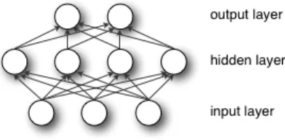
Figure 2.1: Graphical depiction of a one layer neural network (DNN). Image reproduced from

Bengio(2009b).

2.1 Deep neural networks

A deep neural network is the combination of a logistic regressor with a learnt non-linear feature transform Ψ. This approach alleviates the problem of having to extract meaningful features through hand-crafting or off-the-shelf methods. The feature transform Ψ is learnt so that the it makes the input more linearly separable. The feature transform Ψ can be thought of as stack of logistic regressors where the targets are not known. The output units of these intermediary logistic regressions are known as hidden units because of this. A process known as back-propagation is used to propagate down the error from the top logistic regressors whose labels are known to the ones in the feature transform Ψ. This will cause the hidden units to help decrease the overall error of the network.

A single hidden layer neural network (illustrated in Figure 2.1) is typically characterized by the following equations

h1(x) = ψ1(W1x + b1) o(h) = ψ2(W2h + b2)

The parameters W1_{, W}2 _{are called the weight matrices. They represent patterns}

the hidden units are sensitive to and b1_{, b}2 _{are offsets. The dot product is used}

to measure the distance between these patterns and the input. A unit will be strongly activated if the input is strongly co-linear with the pattern in it’s weight vector (with the right offset).

The so-called activation functions ψ1, ψ2are non-linear element-wise scalar

func-tions that control the behaviour of the unit. Without these non-linear funcfunc-tions (ψ1(x) = x) the dot products could be collapsed and the resulting input to

(24)

network to learn non-linear functions of its input. Popular choices are the logistic sigmoid (_1+e1−x), the tanh, and the rectified linear unit (max(0, x)) (Glorot et al.,

2011a). It is common to train networks with the logistic sigmoid as the activation for hidden units ψ1 but several papers have reported better performance using the

rectified linear units Glorot et al. (2011a); Hinton et al. (2012). Finding and jus-tifying activation functions for the hidden layers is still an open research subject (Goodfellow et al.,2013).

The output activation function ψ2 could be any function but the choice is

typi-cally guided by the type of the targets. For regression problems a linear activation is often used (ψ2(x) = x). As we shall see this is justified in some cases because

the network predicts the mean of a gaussian. For 1-of-k classification problems a softmax function is used. The softmax is defined by the following function

p(yk|xi) =

exk

P

jexj

The output is a proper probability because the normalization factor over classes ensures thatP

p(yk|h) = 1. As we shall see, combined with the proper loss function,

the probabilistic justification is that we are learning a multinomial distribution over the labels.

2.1.1 Approximation power

In a one layer network the feature transform Ψ is represented by the function

h1. We can add hidden layers by feeding h1 as input to another hidden layer h2

with different parameters and feeding h2 to the output layer. A one hidden layer

network is a universal approximator Hornik et al. (1989). Given enough hidden units, it can approximate any function. Adding hidden layers will help the network learn functions more efficiently. If the function to be learned can be factorized into sub-procedures then a deeper neural network will be exponentially smaller then it’s shallow counterpart (Delalleau and Bengio, 2011;Pascanu et al., 2014).

2.1.2 The power of distributed representations

The representation Ψ learned by the DNN can be quite powerful. To better understand why, we can compare with an algorithm like Gaussian mixture models

(25)

(GMM). In the GMM, the feature representation Ψ describes how well the example matches each Gaussian of the mixture. The class of the example is affected mostly by the closest mean. Thus we can say that a GMM with N means and O(N ) parameters partitions the space into N sections.

In comparison, the hidden units forming Ψ are like logistic regressions but none of the output units are mutually exclusive. Each unit in Ψ partitions the space independently into two partitions. These binary partitions give rise to many others through combinations. Thus a DNN with N hidden units and O(N ) parameters partitions the input space into 2N _{partitions. This allows the DNN to encode the}

properties of the examples by disentangling factors of variation (Bengio, 2009b). Disentangling the factors of variation means encoding each factor of variation in a different dimension of Ψ. This will allow classification on a specific property or a combination of them to be a linear operation in the space Ψ. The advantage of such a representation is that it would be more compact and would allow for better classification results.

Remarkably, disentangling factors of variation allows non-local generalization. Generalization in local methods like k-NN and decision trees is done by extrap-olating from nearby examples. Local methods cannot generalize to zones in the input space that are far from training examples. With non-local generalization the network can properly operate with unseen examples. It is made possible because the network identifies properties or subspaces where the unseen example may be similar to the training examples. For example, a network may never have seen an example of a blue dog, but if the network disentangles the color from the object, the output logistic can properly classify the example as a dog.

2.1.3 Practical details

The weight matrices W ∈ Rm×n can be initialized with a uniform distribu-tion [−q_m+n6 ,q_m+n6 ] for tanh activation units and ReLU units Glorot and Bengio

(2010). This initialization will ensure that early during training the gradients have zero-mean and unit standard deviation which will make it faster LeCun et al.

(1998).

For regression, the loss function is usually the mean-squared error (MSE) L(x, y) = ky − o(h1(x))k2

(26)

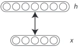
Figure 2.2: Graphical model of the restricted Boltzmann machine (RBM). Image reproduced fromBengio(2009b).

when the targets y are continuous unnormalized values. Combined with a linear output layer this amounts to predict the means of a gaussian. The loss function used for binomial probability vectors is the cross-entropy

L(x, y) = −yT _{log o(h}

1(x)) − (1 − yT) log(1 − o(h1(x)))

where y is a binary vector. If the activation of the output layer is a softmax,

o(h1(x)) will learn the conditional p(yi = 1|x). The gradients for the output

logistic regression is the same as the gradient for a regular logistic regression. The gradients for the hiddens layers are found using the chain rule (Rumelhart et al.,

1986).

Deep neural nets are prone to overfitting because they can learn highly non-linear functions. An advance in regularization (Hinton et al., 2006a;Bengio et al.,

2007a) has created a surge in interest for these models. Another cause of this resurgence is the appearance of fast graphical processing units (GPUs) that can run DNNs very fast.

2.2 Restricted Boltzmann machines

A restricted Boltzmann machine (RBM) is an undirected graphical model with binary variables (Hinton et al., 2006b): observed variables x and hidden variables h. It is defined by the joint probability over {x, h}

P (x, h) = e

−E(x,h)

P

x0_,h0e−E(x

(27)

where the energy function E is given by

−E(x, h) = hT_{Wx + b}T_{h + c}T_x

with parameters θ = (W, b, c).

The Boltzmann machine is one of the first so-called generative models. The idea is to fit the parameters of the distribution P (x, h) so that they correspond to a real-world distribution of interest. We can then generate new examples from the model using sampling techniques like Gibbs sampling. It can also be used to answer questions about the distribution using its conditional distributions.

The distinguishing characteristic of the RBM is the presence of non-linear hid-den units h. It is these units that make the RBM one of the most powerful gen-erative models (Salakhutdinov and Murray, 2008). The hidden units of the RBM can learn to represent hidden factors at play in the distribution. In images for example, it is clear that nearby pixels are related but the relation between distant pixels is quite complicated. A model that only incorporates interactions between visible variables would fail to capture these distant interactions. Instead, the RBM is able to detect edges and object parts as hidden factors that cause the activation of the pixels. These hidden factors can be thought of abstract conditions that are entangled to create what is captured by the visible units.

2.2.1 Conditionals

The restricted Boltzmann machine is distinguished from the Boltzmann machine by the lack of connections inside the set of visible units, and similarly for the hiddens. This gives the RBM closed-form conditionals which can be computed quite efficiently. This limitation does not prevent the RBM from being a universal approximator Le Roux and Bengio (2010).

The conditional distributions over observed and hidden variables are

P (hj = 1|x) = σ( X i Wjixi+ bj) P (vi = 1|h) = σ( X j Wjihj+ ci)

(28)

where m is the number of latent factors and n the number of visibles.

These conditionals are the base of inference in this model. We can use the RBM has a feature extractor through P (h|x). We can generate from the model by combining P (h|x) and P (x|h) with block Gibbs MCMC, described below.

2.2.2 Sampling

It is possible to sample new examples from the learned distribution P (x). This is particularly useful for learning as we will see, but it also has practical applica-tions Bengio et al. (2013). Samples are obtained by running a Markov chain to convergence. Typically the Gibbs sampling transition operator is used.

Gibbs sampling over a distribution X = (X1, . . . , XN) iterates over N sampling

subsets of Xi ∼ P (Xi|X−i) where X−i includes all the variables but the one at

index i. This process is guaranteed to converge to the distribution on X (Bishop,

2006).

For the RBM, we can reduce the number of sampling sub-steps from N to 2 because there are two independent groups of units. We have for the visibles

P (xi|x−i, h) = P (xi|h) and similarly for the hiddens. Sampling is done by

alter-nating between P (h|x) and P (x|h). This process is known as block Gibbs sampling because we are sampling blocks of variables at a time.

A step in the Markov chain is given by ht+1 ∼ P (h|xt) xt+1 ∼ P (x|ht+1₎

We can obtain a sample by iterating these steps until convergence which is guar-anteed for t = ∞. In practice, a small number is steps is enough to reach the stationary distribution.

2.2.3 Learning

There are several principles that can be used to estimate the parameters of the RBM. These methods rely on different inductive principles, but the guiding prin-ciple is to match certain statistics of the target distribution and of the distribution of the model.

(29)

Stochastic maximum likelihood

The classic way of training this model is through maximum likelihood. This re-quires an expression for the likelihood of a sample. It can be found by marginalizing analytically over h to obtain

P (x) = e

−F (x)

P

x0e−F (x

0₎

where the free energy F has the expression −F (x) = cTx +X

j

log(1 + ePiWjixi+bj)

Training the model is in principle as simple as following the gradient of the negative log-likelihood −∂ log P (x) ∂θ = Edata " ∂F (x) ∂θ # − Emodel " ∂F (x) ∂θ #

However, this gradient is intractable because the second expectation is combina-torial. Stochastic Maximum Likelihood or SML (Younes, 1999; Tieleman, 2008) estimates this expectation using sample averages taken from a persistent MCMC chain (Tieleman, 2008). Starting from xi _{a step in this chain is taken by sampling}

hi _{∼ P (h|x}i_{), then we have x}i+1 _{∼ P (x|h}i_{). SML-k is the variant where k is the}

number of steps between parameter updates, with SML-1 being the simplest and most common choice, although better results (at greater computational expense) can be achieved with more steps.

Training the RBM using SML-1 is on the order of O(dn) per update where d is the dimension of the input variables and n is the number of hidden variables. In the case of high-dimensional sparse vectors with p non-zeros, SML does not take advantage of the sparsity. More precisely, sampling P (h|x) (inference) can take advantage of sparsity and costs O(pn) computations while “reconstruction”, i.e., sampling from P (x|h) requires O(dn) computations. Thus scaling to larger input sizes n yields a linear increase in training time even if the number of non-zeros p in the input remains constant.

(30)

Ratio matching

Ratio matching (Hyv¨arinen, 2007) is an estimation method for statistical mod-els where the normalization constant is not known. It is similar to score matching (Hyv¨arinen,2005) but applied on discrete data whereas score matching is limited to continuous inputs, and both are computationally simple and yield consistent esti-mators. Score matching estimates the parameters by matching the local directions of maximum likelihood near input points. The use of Ratio Matching in RBMs is of particular interest because their normalization constant is computationally intractable.

The core idea of ratio matching is to match ratios of probabilities between the data and the model. Thus Hyv¨arinen (2007) proposes to minimize the following objective function Px(x) d X i=1 " g Px(x) Px(¯xi) ! − g P (x) P (¯xi₎ !#2 + " g Px(¯x i₎ Px(x) ! − g P (¯x i₎ P (x) !#2 (2.1)

where Px is the true probability distribution, P the distribution defined by the

model, g(x) = _1+x1 is an activation function and ¯xi _{= (x}

1, x2, . . . , 1 − xi, . . . , xd). In

this form, we can see the similarity between score matching and ratio matching. The normalization constant is canceled because _{P (¯}P (x)_xi₎ =

e−F (x)

e−F (¯xi), however this objective

requires access to the true distribution Px which is rarely available.

Hyv¨arinen (2007) shows that the Ratio Matching (RM) objective can be sim-plified up to constants in θ to JRM(x) = d X i=1 g P (x) P (¯xi₎ !!2 (2.2)

which does not require knowledge of the true distribution Px. This objective can

be described as ensuring that the training example x has the highest probability in the neighborhood of points at hamming distance 1.

In Chapter 6 we prove that one can rewrite Eq. 2.2 in a form reminiscent of auto-encoders: JRM(x) = d X i=1 (xi− P (xi = 1|x−i))2. (2.3)

(31)

auto-encoders is that each input variable is predicted by excluding it from the input.

Applying Equation2.2to the RBM we obtain JRM(x) =Pdi=1(σ(F (x) − F (¯xi)))

2

. The gradients have the familiar form

−∂JRM(x) ∂θ = d X i=1 2ηi " ∂F (x) ∂θ − ∂F (¯xi₎ ∂θ # (2.4) with ηi = (σ(F (x) − F (¯xi))) 2 − (σ(F (x) − F (¯xi₎₎₎3_.

A naive implementation of this objective is O(d2n) because it requires d

com-putations of the free energy per example. This is much more expensive than SML, as noted by Marlin et al. (2010). Thankfully, as we argue here, it is pos-sible to greatly reduce this complexity by reusing computation and taking advan-tage of the parametrization of RBMs. This can be done by saving the results of the computations α = cT_{x and β}

j = PiWjixi + bj when computing F (x).

The computation of F (¯xi_{) can be reduced to O(n) with the formula −F (¯}_xi_{) =}

α − (2xi− 1)ci+Pjlog(1 + eβj−(2xi−1)Wji). This implementation is O(dn) which is

the same complexity as SML. However, like SML, RM does not take advantage of sparsity in the input.

2.3 Regularized auto-encoders

A regularized auto-encoder (AE) is a feed-forward neural network trained to reconstruct its input. The original insight of the auto-encoder is that by rebuilding the input you use the input as the teaching signal in gradient descent. However, simply learning does not guarantee that the model will learn interesting patterns in the data. Classical auto-encoders limit the capacity by setting the number of latent factors below the dimension of the input, forming an under-complete representa-tion. This restricted the model to learning a subspace of the principal components (Bourlard and Kamp, 1988). Recently, several models have been using different forms of regularization that allow learning richer features from the input (Vincent et al., 2010; Rifai et al., 2011). Notably these regularizers allow learning over-complete representations which have more features than inputs. Unlike RBMs the

(32)

AEs are not primarly motivated by probabilistic modelling. However, a recent line of papersVincent(2011);Rifai et al.(2012);Alain and Bengio(2013) (one of which I’ve co-authored) has shown that regularized auto-encoders have a probabilistic in-terpretation.

2.3.1 Denoising auto-encoders

The DAE is a learning algorithm for unsupervised feature extraction Vincent et al. (2010): it is provided with a stochastically corrupted input and trained to reconstruct the original clean input. Its training criterion can be shown to relate to several training criteria for density models of the input through Score Matching Hyv¨arinen (2005); Vincent (2011). It is also possible to show that the denoising objective yields to learning about the data distribution by using local moments and learning the score (Alain and Bengio,2013). Alain and Bengio(2013) shows that the difference vector between the reconstruction and the input is the model’s guess as to the direction of greatest increase in the likelihood, whereas the difference vector between the noisy corrupted input and the clean original is nature’s hint of a direction of greatest increase in likelihood (since a noisy version of a training example is very likely to have a much lower probability under the data generating distribution than the original). It can also be shown that the DAE is extracting a representation that tries to preserve as much as possible of the information in the input (Vincent et al., 2010).

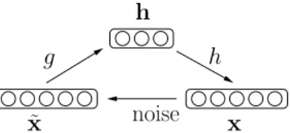
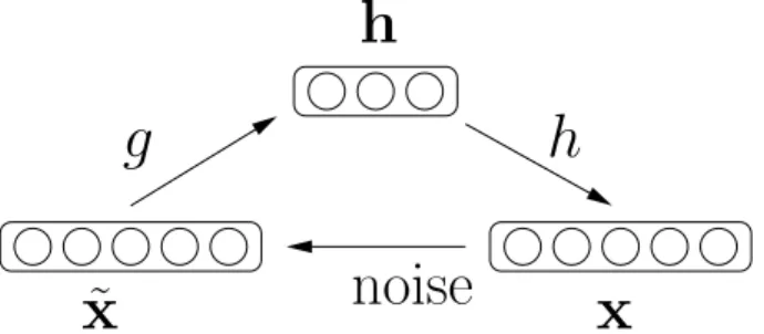
noise g ˜ x x h h

Figure 2.3: Schematic of the Denoising Auto-Encoder

The denoising auto-encoder reconstruction f (x) = h(g(x)) is composed of an encoder function g(·) and a decoder function h(·) (see Figure2.3). During training, the input vector x ∈ [0, 1]d _{is partially and randomly corrupted into the vector ˜}_x.

The encoder takes ˜x and maps it into a hidden representation h ∈ [0, 1]d0_{. The}

decoder takes the representation h and maps it back to a vector z in the input space ([0, 1]d _{in our case). The DAE is trained to map a corrupted input ˜}_{x into the}

(33)

original input x such that g(h(˜x)) ≈ x. This forces the code h to capture important and robust features of x. Many corruption processes are possible, but they should have the property of generally producing less plausible examples. Typically, inputs are corrupted by randomly setting elements of x to 0 or 1, or adding Gaussian noise. The typical shallow encoder has the form

a1 = W(1)· ˜x + b(1)

h = s1(a1) (2.5)

where sa is a non-linear function like the sigmoid sa(u) = 1/(1 + exp(−u)), W(1)

is a d0× d weight matrix and b(1) _{is a d}0_{× 1 vector. The function computed by the}

decoder is

a2 = W(2)· h + b(2)

z = s2(a2) (2.6)

Where W(2) _{is a d × d}0 _{weight matrix and b}(2) _{is a d × 1 vector.}

Training

Given a dataset Dn = (x(1), x(2), . . . , x(n)), the parameters (W(1), b(1), W(2),

b(2)_{) are trained by stochastic gradient descent to minimize a negative log-likelihood}

ˆ R(f, Dn) = 1 n n X i

− log p(x(i)|f (˜x(i)) = 1

n

X

i

d(x(i), f (˜x(i)))

where d is a measure of the log-likelihood.

The measure that is typically used for binary vectors or vectors of binomial probabilities is the cross-entropy (or Bernouilli log-likelihood).

d(x, z) = −

d

X

k

[xklogzk+ (1 − xk)log(1 − zk)]

The L2 distance is preferred when the input is continuous and without bounds because it corresponds to a Gaussian log-likelihood:

(34)

The training updates of the denoising auto-encoder with a single layer neural net is in O(mn) where m is the dimension of the input and n the number of hidden units.

The noise distribution is chosen through cross-validation. In most cases the binomial distribution will lead to better performance for binary vectors and the Gaussian will work better for continuous inputs. The level of the noise is an im-portant hyper-parameter in this model. Theory (Alain and Bengio,2013) suggests that the score is best estimated with a small noise but in practice the noise levels are quite high. Typical values for the probability the binomial corruption are be-tween 0 and 1, and the optimal standard deviation when using gaussian noise is also usually found between 0 and 1.

Justification as a generative model

Vincent (2011) showed that a particular parametrization of the denoising auto-encoder is equivalent to the application of score matching of to a particular gen-erative model. The connection was quite brittle but it planted the idea that the DAE could have a proper theoretical justification. The link was also interesting because it shed light on what is captured by the DAE to model the distribution. Score matching (Hyv¨arinen, 2005) is a parameter estimation method that relies on matching a local statistic called the score ∂ log p(x)_∂x between the model distribution and the data distribution. The score indicates the direction of highest likelihood increase around the example. The link to score matching is evidence towards the idea that the simple and efficient denoising objective learns the directions of highest likelihoods.

Alain and Bengio(2013) establishes a more general link between denoising auto-encoders and generative models. Assuming only small noise and a mean squared error reconstruction, they show that after training the score is given by

∂ log p(x)

∂x =

r(x) − x

σ2 + O(σ 2₎

The probability distribution can be recovered by integrating over the score. In practice this is inefficient, but recovering the distribution is not required to use the DAE has a feature extractor. Bengio et al.(2013) further generalized these results to arbitrary noise and arbitrary parametrization of the denoising auto-encoder.

(35)

2.3.2 Contractive auto-encoders

The contractive auto-encoder (Rifai et al., 2011) (CAE) is an unsupervised learning algorithm for feature extraction which uses a Tikhonov regularization (Tikhonov and Arsenin, 1977) on the learned features. The regularization helps achieve robust features that have been found to reach state-of-the-art performance on several benchmarks (Rifai et al., 2011,2012). The CAE learns about the input distribution by capturing the local directions of variations around the input points. The CAE comprises an encoder function

h = h(x) = σ(W · x + b(1)) and a decoder function

z = r(h) = σ(WT · h + b(2)).

The distinctive characteristic of the CAE is that the loss combines the recon-struction error with a penalty on the Frobenius norm of the Jacobian of the hidden mapping ˆ R(f, Dn) = 1 n n X i d(x(i), r(h(x(i)))) + λ ∂h(x(i)₎ ∂x(i) 2 .

The hyper-parameter λ is to be cross-validated and optimal values are typically within 0 and 1. The training objective is in O(mn) where m is the dimension of the input and n the number of hidden units.

The CAE captures information about the input through the two opposing forces in its loss function. The reconstruction is a term that guarantees that features conserve information about the input. It can be thought of as a soft way to ensure the encoder is a bijective mapping (Le et al., 2011), at least near the training examples. The Jacobian penalty encourages the model to be invariant and in the limit with λ → ∞ it would force the model to learn a constant feature mapping. The Jacobian penalty is known as contractive and gives the model its name.

The Jacobian measures the variation of each hidden unit with respect to vari-ations in the input ∂hi

∂xi = hi(1 − hi)Wij. Minizing this variation can be achieved

either by saturating the hidden units (setting them close to 0 or 1) or reducing the norm of the weights. However, the CAE cannot simply reduce the norm of

(36)

the weights because the same weights are used for encoding and decoding. This is known as tied weights. The model must therefore learn to saturate and ignore certain variations in the input.

The contraction forces the model to discard as many directions of variations as possible. The reconstruction forces the model to keep the directions that occur in the data. The result is that the features hi(x) are only sensitive to directions

in the input that actually occur in the data. (Rifai et al., 2011) has shown that these correpond to tangents of the data manifold. The tangents can be recovered by an eigen-decomposition of the Jacobian where the eigen-vectors with non-zero eigen-values are the local tangents at that point. As we will show in Chapter8this insight can be used to further regularize a deep neural network.

2.3.3 Links between auto-encoders and RBMs

RBMs have generally been preferred to auto-encoders because they have more theoretical justification. However, the auto-encoders are generally simpler to un-derstand and implement. A simple look at the conditionals of the RBM and the encoder/decoder of the AEs suggest that the models are similar in some way. Elu-cidating the links between these two model families has been the subject of several papers Bengio and Delalleau (2009); Vincent (2011); Alain and Bengio (2013);

Swersky et al. (2011).

Vincent (2010); Alain and Bengio (2013) have confirmed the intuition that certain auto-encoders capture the probability distribution through local statistics. This result is generalized by Bengio et al. (2013) who shows that auto-encoders with arbitrary noise and arbitrary parametrizations are generative models. This constitutes a very flexible framework for generative models.

Swersky et al. (2011) has shown that applying score matching to any parame-terization of an RBM will lead to an auto-encoder. This encourages a new way to approach modeling with unsupervised models. The probabilistic framework of the RBM can be used to reason about the models but they can be implemented simply by transforming them into auto-encoder form using score matching.

(37)

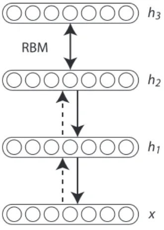
Figure 2.4: Graphical model of the deep belief network (DBN). Image reproduced fromBengio

(2009b).

2.4 Stacking RBMs and AEs

The RBMs and AEs form basic learning modules that can be stacked to create deep architectures (Hinton et al., 2006a; Bengio et al., 2007a). Stacking these feature extractors will allow each layer to gradually learn more abstract features. Experiments have shown that these more abstract features can be useful on several classification problems (Le et al., 2012;Dahl et al., 2012).

Traditionally a feature extraction pipeline will include many layers of hand-crafted or off-the-shelf features. Popular off-the-shelf features for vision include SIFT (Lowe, 1999) for example. One ground-breaking idea pioneered by Hinton et al. (2006a); Bengio et al. (2007a) is to learn these features automatically using unsupervised data which is often easy to obtain. These features will have the advantage of being more tuned to the data and often the classification task. A paper which I’ve co-authored (Bengio et al.,2013) also shows deep algorithms lead to better mixing during sampling.

2.4.1 Deep belief nets

Stacking RBMs leads to a generative model called the deep belief net (DBN). The training algorithm is a greedy iterative procedure. The RBM at layer l is trained on pseudo-data sampled from the posterior p(h|x) of the model at layer

(38)

l − 1. This results in the following generative model p(v, h(1), · · · , h(L)) = "_L−1 Y l=1 p(h(l−1)|h(l)) # p(h(L−1), h(L)).

Surprisingly this model combines both directed and undirected connections even though the basic RBM is undirected (Figure 2.4). The last layer has undirected connections while the other layers are directed top-down. Exact inference in the model is intractable because of the depth and the presence of the directed con-nections. The features can be extracted by propagating the posterior over hiddens upward in the model. Hinton et al.(2006a) suggest using the last layer of the DBN as features or using the DBN to pretrain a deep neural network. In the case of pretraining, the parameters of the trained DBN are used as a starting point for the optimization of the DNN.

2.4.2 Stacked auto-encoders

Recent work (Bengio et al., 2007a; Vincent et al., 2010; Rifai et al., 2011) has shown that several regularized auto-encoders can take advantage of depth. The earliest work (Bengio et al., 2007a) generalizes the result of (Hinton et al., 2006a) with RBMs to classical auto-encoders. Even without regularization the classical auto-encoder trained with a greedy layer-wise fashion is able to reduce the error on MNIST from 2.4% to 1.4%Bengio et al.(2007a). In most work with auto-encoders (Bengio et al., 2007a; Vincent et al., 2010; Rifai et al., 2011) a greedy layer-wise scheme is used to obtain a deep architecture. This means training an auto-encoder at layer l on the representation learned by the auto-encoder at layer l − 1. There has been interest for deep auto-encoders that are trained globally but this is still an open research area. A difficulty of this approach is that of optimizing such a deep auto-encoder.

2.5 Why does pretraining work?

Experiments have shown that pretraining helps mainly as a regularizer and as an aid to optimization to some extent (Erhan et al., 2010). As a regularization,

(39)

the prior enforced by pretraining is that the supervised task is based on the factors that explain some of the variations salient in the input data. In traditional machine learning, we assume the targets are directly related to the observations and we model this directly. In the case of pretraining for supervised tasks, we assume both the observations and the targets are caused by latent factors. In this framework, it makes sense to model the latent factors. Moreover, the targets are typically one-hot vectors which convey little information about the patterns to be detected. Learning the distribution of the observation has the benefit of being very rich in information because the targets are dense vectors. This allows the unsupervised model to quickly recover the latent factors (Erhan et al.,2010). When the parameters of the unsupervised model are used to initialize a neural network they set it up in a local basin of attraction. The pretraining process will saturate the hidden units making it more difficult to move far in optimization space. This will force the optimizer to seek a minimum that is close to the initialization (Erhan et al., 2010). Some evidence suggests that pretraining is also useful to optimization (Erhan et al.,2010). However, my experiments on datasets larger than those considered in (Erhan et al.,

2010) have shown that pretraining does not help in these regimes (over 1 billion examples), which contradicts the notion that it helps optimization.

2.6 Beyond pretraining

Glorot et al.(2011a) has gone beyond the breakthrough of (Hinton et al.,2006a;

Bengio et al., 2007a) by showing yet another way to train deep neural nets. It is a sizeable departure from both (Hinton et al.,2006a; Bengio et al.,2007a) because it does not rely on unsupervised pretraining in any way. This makes the approach simpler to use for practitioners and more applicable to very large-scale labeled datasets. Glorot et al. (2011a) shows that DNN with ReLU activation units can be trained without layer-wise pretraining. Hinton et al. (2012) further explores this direction using a new regularization. The idea is to set with probability p a random subset of the hidden units to 0 during the training of the DNN. At test time, the parameters are divided by p as a correction. This procedure helps to fight co-adaptation in the hidden units. Another explanation proposed by (Hinton et al., 2012) is that dropout is an efficient way to do bagging with an exponential

Advances in scaling deep learning algorithms

Résumé

Summary

Contents

List of Figures

List of Tables

List of Abbreviations

Acknowledgments

1

Introduction

1.1

Introduction to machine learning

1.2

Model families

1.3

Optimization

1.4

Regularization

1.5

Supervised Learning

1.5.1

Naive Bayes

1.5.2

Logistic regression

1.5.3

Deep Neural Networks

1.6

Unsupervised Learning

2

Deep Learning

2.1

Deep neural networks

2.1.1

Approximation power

2.1.2

The power of distributed representations

2.1.3

Practical details

2.2

Restricted Boltzmann machines

2.2.1

Conditionals

2.2.2

Sampling

2.2.3

Learning

2.3

Regularized auto-encoders

2.3.1

Denoising auto-encoders

2.3.2

Contractive auto-encoders

2.3.3

Links between auto-encoders and RBMs

2.4

Stacking RBMs and AEs

2.4.1

Deep belief nets

2.4.2

Stacked auto-encoders

2.5

Why does pretraining work?

2.6

Beyond pretraining