HAL Id: hal-01431041
https://hal.archives-ouvertes.fr/hal-01431041
Submitted on 10 Jan 2017
HAL is a multi-disciplinary open access
archive for the deposit and dissemination of
sci-entific research documents, whether they are
pub-lished or not. The documents may come from
teaching and research institutions in France or
abroad, or from public or private research centers.
L’archive ouverte pluridisciplinaire HAL, est
destinée au dépôt et à la diffusion de documents
scientifiques de niveau recherche, publiés ou non,
émanant des établissements d’enseignement et de
recherche français ou étrangers, des laboratoires
publics ou privés.
The viscous curtain: General formulation and
finite-element solution for the stability of flowing viscous
sheets
C Perdigou, Basile Audoly
To cite this version:
C Perdigou, Basile Audoly. The viscous curtain: General formulation and finite-element solution for
the stability of flowing viscous sheets. Journal of the Mechanics and Physics of Solids, Elsevier, 2016,
96, pp.291 - 311. �10.1016/j.jmps.2016.07.015�. �hal-01431041�
The viscous curtain:
general formulation and finite-element solution
for the stability of flowing viscous sheets
C. Perdigoua, B. Audolya,b
aUPMC Univ Paris 06, CNRS, UMR 7190, Institut Jean Le Rond d’Alembert, F-75005 Paris, France
bLMS, ´Ecole Polytechnique, CNRS, Universit´e Paris-Saclay, 91128 Palaiseau, France
Abstract
The stability of thin viscous sheets has been studied so far in the special case where the base flow possesses a direction of invariance: the linear stability is then governed by an ordinary di↵erential equation. We propose a mathematical formulation and a numerical method of solution that are applicable to the linear stability analysis of viscous sheets possessing no particular symmetry. The linear stability problem is formulated as a non-Hermitian eigenvalue problem in a 2D domain and is solved numerically using the finite-element method. Specifically, we consider the case of a viscous sheet in an open flow, which falls in a bath of fluid; the sheet is mildly stretched by gravity and the flow can become unstable by ‘curtain’ modes. The growth rates of these modes are calculated as a function of the fluid parameters and of the geometry, and a phase diagram is obtained. A transition is reported between a buckling mode (static bifurcation) and an oscillatory mode (Hopf bifurcation). The e↵ect of surface tension is discussed.
Keywords: A. Buckling, B. Plates, C. Stability and bifurcation
1. Introduction
The buckling of viscous sheets is involved in a number of phenomena encompassing diverse length and time scales. In earth sciences, viscous shell models have been used to capture the periodic buckling of the subducted lithosphere on geological time scales by Ribe et al. (2007). A number of industrial processes involve thin viscous layers undergoing large deformations: in the float glass process introduced by Pilkington (1969), for example, a thin layer of molten glass floating on a bath of tin is stretched to produce thin glass panels, and the process is controlled so as to avoid wrinkling instabilities (Pfingstag et al., 2011). In the food industry, the folding instability of a viscous sheet, such as hot chocolate or liquid ice cream, impinging a surface is commonly used to produce regular, decorating folds—a technique well-known to pastry enthusiasts. In fluid mechanics, the burst of a bubble near the surface of a viscous fluid involves the collapse of a thin spherical viscous film; the wrinkles formed by this collapse have been studied by Debr´egeas (1998); da Silveira et al. (2000). A similar experiment has been studied by Boudaoud and Cha¨ıeb (2001) where a small viscous disk at the surface of water is poked and forms wrinkles due to hoop stresses.
A classical experiment involving a sheared viscous sheet in an axisymmetric geometry has provided a powerful motivation for subsequent theoretical work on the stability on thin viscous shells. Taylor (1958) first experimented with a thin layer of viscous fluid floating on a denser fluid in an annular region enclosed between a rotating inner disk and a fixed outer cylinder, and reported wrinkles in the viscous sheet produced by the shear flow. A number of studies have analyzed this specific geometry in more detail, with the aim of characterizing the instability. Suleiman and Munson (1981) proposed a quantitative version of the experiment, and identified the dimensionless shear stress governing buckling. Benjamin and Mullin (1988) argue that thin shell models are inapplicable for this particular problem, and analyze the instability based on the equations for 3D viscous flows. Slim et al. (2012) simplify the geometry by addressing an infinite viscous strip sheared by lateral walls; they modify the thin viscous shell model to include an advection
term, and argue that the modified model captures the wrinkling instabilities more accurately. Bhattacharya et al. (2013) analyze again the stability of a sheared annular floating viscous sheet, based on a thin shell model; while they obtain good agreement with their experiments in some range of the parameters, they also point out the shortcomings of the shell model which for very thin sheets predicts very short wavelength instabilities, and a vanishingly small buckling threshold. Ribe (2012) emphasizes that even the inclusion of surface tension would not cure these shortcomings.
These stability analyses are all concerned with base flows possessing a direction of invariance, such as the axisymmetric geometry of Taylor (1958) or the infinite strip of Slim et al. (2012). In the presence of such symmetries the stability is essentially a 1D problem; it can be expressed mathematically as an eigenvalue problem for an ordinary di↵erential equation. In this paper, we address the general case of a base flow possessing no direction of invariance: the eigenvalue problem governing stability is then formulated on a genuinely 2D domain and it involves partial di↵erential equations. A numerical solution of the linear stability analysis is proposed based on the finite element method. To do so, we build up on the methods used for analyzing the stability of elastic plates, a mature field in which non-invariant base solutions are routinely addressed, see the work of Friedl et al. (2000); Zheng (2009); Healey et al. (2013); we also build up on the classical numerical methods for the stability dissipative bulk materials (Triantafyllidis and Leroy, 1994). A specificity of the annular geometry studied in previous work is that the fluid trajectories are closed and periodic; by contrast, we address the more general case of an open flow, i.e. with fluid elements continuously entering and exiting the domain.
The main goal of this paper is to introduce the mathematical formulation and the simulation tools that allow one to address the stability of thin viscous sheets in arbitrary geometries. Viscous sheets have been much less studied than one-dimensional viscous filaments, for which mechanical models, stability analyses and numerical methods are available (Entov and Yarin, 1984; Teichman and Mahadevan, 2003; Ribe, 2004; Bergou et al., 2010; Arne et al., 2015).
As an illustration of viscous flows possessing no direction of invariance, we propose and analyze a problem inspired by a glass forming process patented by Dockerty (1967). A gutter is filled with molten glass, which overflows and forms a thin sheet of glass stretched by gravity. The glass cools down and glass panels are cut o↵ at the bottom. Accordingly, we study the flow in a thin viscous sheet produced by injecting fluid at a horizontal slit with prescribed velocity, the sheet being stretched by gravity as it falls in a bath of fluid placed below, see figure 1. We ignore thermal e↵ects and assume that the fluid viscosity is homogeneous. As the sheet flows, an in-plane viscous stress appears. We analyze the possibility that the sheet buckles when the stress is compressive. This system is therefore the viscous analogue of the well-studied wrinkled elastic membrane under traction, see the work of Friedl et al. (2000); Cerda et al. (2002); Zheng (2009); Healey et al. (2013).
Our stability analysis is based on the viscous sheet model, a 2D model for the viscous fluid akin to plate models for elastic materials. For this 2D model to be applicable, the velocity and thickness in the base state must vary over a length scale much larger than the thickness, and the velocity must be nearly constant across the thickness. The derivation of viscous sheet models from the 3D equations for Stokean fluid is well documented in the literature; a short review is given in§2 below.
The outline of the paper is as follows. In§2 the viscous sheet model is introduced; equivalent formulations of the equations for the balance of viscous stress are proposed, both in strong form (local stress balance) and in weak form (principle of virtual work). In §3, these equations are solved in a planar geometry assuming that the flow is stationary: this yields the base state of our viscous buckling problem. The buckling modes are obtained numerically in§4 by a linear stability analysis. In §5, the e↵ect of surface tension is included and its stabilizing e↵ect on the curtain modes is discussed.
2. Model for a falling viscous sheet
In this section we present the mathematical model governing the motion of a thin viscous sheet poured from a horizontal slit, which is stretched by gravity and falls in a bath of fluid. The motion in the sheet is governed by the balance of viscous stress, including both stretching and bending stress, as well as by gravity
Figure 1: Thin viscous sheet stretched by gravity and falling into a bath of fluid.
and surface tension. The general, non-linear equations of motion derived in this section will be specialized to the case of a steady planar flow for the calculation of the base solution in §3, and later linearized near this base solution in§4.
2.1. Notations and assumptions
We use Cartesian coordinates (x, y, z), as depicted in figure 1: the x axis is in the vertical direction and oriented downwards, the y axis is along the direction of the slit (i.e. across the width of the sheet), the z axis is perpendicular to the sheet. The orthonormal Cartesian basis is denoted by (ex, ey, ez). We shall use a two-dimensional model for the sheet based on the theory of thin viscous plates: at time t, a generic point on the midsurface of the sheet is labelled through its coordinates (x, y)2 DtwhereDtis the domain
obtained by projecting the mid-surface of the sheet onto the (x, y) plane. For the thin sheet model, (x, y) are Eulerian coordinates.
We shall assume throughout this paper that the e↵ect of viscosity is dominant in the sense that velocities remain everywhere close to the injection velocity U ex imposed at the top slit, see equation (17a) below.
As a result, the lateral edges are almost vertical and the width of the sheet is almost constant. Under this assumption of dominant viscosity, one can therefore approximate1 the Eulerian domain with a rectangle
that is independent of time,
Dt= [ H, 0]⇥ [ H, H]. (1)
Here, we denote by H the height of the sheet, i.e. the distance from the slit to the bath, and by H its half-width, i.e. half the length of the slit: the quantity is half the aspect-ratio of the sheet.
The top of the sheet, where the fluid is injected through a slit, corresponds to x = H. The bottom, where the fluid makes contact with the bath at rest, is x = 0. The axis of the sheet is y = 0 and the lateral edges are y = ± H. When symmetries allow, we will restrain our analysis to the half-domain (x, y)2 [ H; 0] ⇥ [0; H] and apply appropriate symmetry conditions on the axis y = 0.
Unless stated otherwise, all unknowns are functions of (t, x, y), even though the dependence on time t is sometimes implicit for the sake of conciseness. Bars below symbols denote tensors, with the number of bars matching their rank (a single bar for vectors such as ex, two for matrices, etc.) A comma in a
subscript indicates partial derivation, as in ,x= @ /@x. We use Einstein’s summation convention, whereby
1A similar simplification arises in problems of linearized elasticity, where there is no need to distinguish between reference
and actual configurations in the arguments of unknown functions. In the viscous case problem studied here, there is no need to distinguish between the actual position of a particle and the position it would have arrived at if it had been advected by the constant and stationary velocity field U ex.
a summation is implied whenever repeated indices appear on the same side of an equality. Greek letters will be used for indices belonging in plane of the sheet: x↵, for example, means x or y, but not z.
Viscous sheet models can be justified by dimensional reduction, starting from the Stokes equations for viscous fluids in 3D in the limit h⌧ H where the thickness h is small compared to the size H of the sheet, see for instance Howell (1996); Ribe (2001, 2002); Pfingstag et al. (2011). Di↵erent models are applicable to viscous sheets, corresponding to di↵erent sets of scaling assumptions. One set of scaling assumptions yields the Trouton model which holds on long time scales, and describes the evolution of the thickness h as a result of stretching; see Filippov and Zheng (2010) for an application. Other sets of assumptions yield a family of models, known as Buckmaster-Nachman-Ting (BNT) models after the work of Buckmaster et al. (1975); Buckmaster and Nachman (1978): BNT models describe the bending of viscous sheets occurring on much shorter time scales. The model we use in this paper is akin to the classical small-deflection BNT model describing the incipient buckling of viscous sheets, as derived by Howell (1996) and applied by Pfingstag et al. (2011) and others. More accurately, the viscous sheet model we use in this paper is identical to the model derived in§2.2 of the paper by Howell (1996) and by Pfingstag et al. (2011) with m = 1 in their notation; in the present work, however, this model is derived from di↵erent scaling assumptions than in the work of Howell and others. These di↵erences are discussed at the end of this paper, in§6.
On the time and force scales addressed by the BNT model, the evolution of thickness is negligible. Our buckling analysis is based on a model in the BNT family. Accordingly, the thickness h is constant along trajectories. For the sake of simplicity2, we assume that the sheet is injected at the top slit with a uniform
thickness: as a result, the thickness h is uniform in the entire domain.
In this paper, the evolution of the sheet is parameterized by the deflection w(x, y, t) of the sheet’s mid-surface (where the deflection is defined as the z-component of the current position), and the in-plane projection of the velocity u(x, y, t) = ux(x, y, t) ex+ uy(x, y, t) ey. A similar set of kinematical variables
is used in the dimensional reduction of Howell (1996). This choice of kinematical variables is well suited to buckling analyses, as we show. As we start from a dimensionally reduced model, the viscous sheet is represented as a surface, parameterized by the Eulerian variables (x, y) and by the time t, whose motion in the 3D Cartesian space is described by its in-plane velocity u and out-of-plane deflection w. It is important to note that we use a velocity u = (ux, uy) in the in-plane direction but a displacement w in the transverse
direction.
We now proceed to introduce the main dimensionless groups associated with the various forces influencing the motion of the sheet. We do so by proposing a qualitative scaling argument, which will guide us later in rescaling the full equations, see§2.5. The surface tension between the liquid and ambient air is assumed to be constant. The volume mass of the sheet is denoted by ⇢, and its dynamic viscosity by µ. Let g be the acceleration of gravity, w⇤ the typical deflection, h the thickness imposed by the slit and H the height of
fall. When expressed per unit volume, the weight and the capillary forces are of order ⇢ g and ( w⇤/H2)/h,
respectively (note that the typical curvature of the sheet is w⇤/H2, which gives rise to a surface density of
capillary force w⇤/H2). We compare these forces to typical force arising from viscosity, per unit volume:
U/H has the dimension3 of a strain rate, µ U/H has the dimension of a viscous stress, and µ U/H2 has the
dimension of a net force per volume (it is given by the divergence of the stress). The ratio of the typical weight to the typical viscous forces is known as Je↵reys’ number (Je↵reys, 1925):
Je = ⇢ g H
2
µ U , (2)
and the ratio of the typical capillary force to the typical viscous force is known as the inverse capillary number,
Ca 1= 2
µ U. (3)
2This assumption could be easily relaxed, as noted in§6.
3The ‘typical’ quantities identified here are simply given as a mean to identify the dimensionless groups relevant to our
problems, and are not meant to be accurate estimates of the true solution. In fact, as we shall see later, the actual shear rates in the sheet are much smaller than the na¨ıve estimate U/H proposed above, by a factor of order Je⌧ 1.
Here, we have assumed that the typical deflection is comparable to the thickness,
w⇤⇠ h. (4)
This classical scaling assumption in fact underlies the derivation of the plate model, see for instance§2.2 in the paper of Howell (1996), or Pfingstag et al. (2011).
Let ⌘ denote the thickness-to-height ratio of the sheet, ⌘ = h
H. (5)
We assume it to be small,
⌘⌧ 1, (6)
as this a necessary condition for the two-dimensional viscous sheet model to be applicable.
As explained above, we assume that the e↵ect of viscosity is dominant compared to that of gravity and capillary forces: the motion of the sheet is close to a vertical downwards rigid-body motion with the velocity U imposed by the injection. In other words we consider the asymptotic limit
Je⌧ 1, Ca 1
⌧ 1. (7)
The asymptotic regime considered in this work is only partially specified by (6) and (7): as shown later on, we shall more specifically consider the distinguished limit Je ⇠ ⌘2 and Ca 1
⇠ ⌘3, which will follow
naturally from the equations of motion of the sheet. In addition, we work in the viscous regime, assuming that Reynolds number is small, Re = ⇢ U H/µ⌧ 1. Accordingly, the motion is governed by a balance of forces, and inertia can be neglected.
2.2. Kinematics
Since our choice of kinematic variables is non-standard, we first need to derive the expression of the strain rate tensor d↵ in terms of the out-of-plane deflection w and of the in-plane velocities u↵. To do so,
we consider the advection of an infinitesimal material segment l tangent to the mid-surface of the sheet, whose endpoints have coordinates (x, y, w(x, y, t)) = (x↵, w(x , t)) and (x + x, y + y, w(x + x, y + y, t)) =
(x↵+ x↵, w(x + x , t)) at time t. Recall that we use Greek indices such as x↵ and x for both
in-plane coordinates x and y; by a slight abuse of notation, we use as a summation index as there is no risk of confusion with the half aspect ratio . Let us denote by D/Dt the convected derivative, i.e. the time derivative obtained by following material points. By definition of the tangent velocity, the in-plane coordinates (x, y) of the first endpoint evolves according to Dx↵
Dt = u↵(x , t). A similar formula
yields the evolution of the other endpoint. Taking the di↵erence, we obtain the evolution of the in-plane projection of the infinitesimal segment as D x↵
Dt = u↵, (x , t) x , where we recall that a comma in subscript
denotes a partial derivative and that there is an implicit sum over the repeated index . The out-of-plane projection of the material segment is z = w,↵(x , t) x↵. Its rate of change is D zDt = DwDt,↵ x↵+ w,↵D xDt↵ =
(w,↵t+ u w,↵ ) x↵+ w,↵u↵, x . With these two formulas, it is possible to calculate the rate of change
of the squared length of the material segment as 1 2 D( l2) Dt = x↵ D x↵ Dt + z D z Dt = x↵ x ⇥ u↵, + w,↵(w, t+ u w, + w, u , )⇤.
To derive the last equality, some dummy indices have been renamed. The symmetric part of the tensor appearing in square brackets is called the membrane strain rate tensor d and satisfies the identity 1
2 D( l2)
Dt =
l· d · l. Its components are found by identification with the above equation as:
d↵ = u(↵, )+ w,(↵w, )t+ u w,(↵w, ) + u ,( w,↵)w, , (8a)
where parentheses in subscripts mean that the enclosed indices must be symmetrized, as in u(↵, )= (u↵, +
where aM = D(a)Dt + a· ru denotes the lower-convected (covariant) time derivative of a vector: this is a co-rotational time derivative, which confirms that the membrane strain rate tensor d is objective. This tensor measures the rate of stretching of the mid-surface of the sheet, and determines the membrane stress via the constitutive laws for viscous stretching, which we will derive in the following section. In the definition (8a) of the membrane strain rate, the first term coming fromru is the classical strain rate tensor for 2D flows, and the other terms coming fromrw ⌦ (rw)Mcapture in-plane strain caused by the (out-of-plane) deflection: a similar geometrical nonlinearity appears in the F¨oppl–von K´arm´an equations for elastic plates, but without any time derivative.
We now proceed to introduce the second measure of strain rate, namely that associated with the rate of change of curvature of the midsurface. The deflection has been assumed to scale like w⇤ ⇠ h ⇠ ⌘ H ⌧ H,
implying that the deflection angle stays small, w,↵ ⇠ w⇤/H ⇠ ⌘ ⌧ 1. As a result, the curvature can
be approximated by the the Hessian of the midsurface, and it reads w,↵ in components and rrw in
tensor notations. We define the curvature strain rate tensor k as the co-rotational derivative of the Hessian, k = (rrw)M, where we have introduced the lower-convected derivative of a second-order tensor as aM =
Da Dt+ru
T
· a + a · ru. In components, the curvature strain rate is therefore defined as
k↵ =D(w,↵ )
Dt + ru
T
↵ rw + rw ↵ ru
= w,↵ t+ u w, ↵ + 2 u ,(↵w, ) . (8b)
The first term w,↵ tis the partial time derivative, the second term u w, ↵ makes it convective, and the last
term 2 u ,(↵w, ) makes it co-rotational with the flow. This last term warrants that the strain rate tensor
k remains zero if the sheet is passively advected by an in-plane velocity u describing a rigid-body rotation. It is included for the sake of completeness even though it plays no role for the linear stability analysis of the particular problem studied here, as confirmed later above equation (26). Finally, we note that other definitions of the co-rotational derivative are possible, such as the Jaumann or upper-convected derivative; these alternative definitions of the tensor k coincide with our particular one when the membrane strain rate is zero (d = 0), and this warrants that the corresponding viscous sheet models are all asymptotically equivalent in the limit of small thickness, as both the viscous bending modulus and the membrane strain rate are small in this limit.
The membrane strain rate tensor d in (8b) has the dimension of the inverse of a time; the curvature strain rate tensor k has the dimension of the inverse of a length, times the inverse of a time.
Having specified the strain rate measures relevant to our viscous sheet model, we proceed to write down the constitutive relations and the expressions for the virtual works.
2.3. Constitutive relations for viscous sheets
In a thin plate, the state of stress is described by a membrane stress tensor N and bending moment tensor M . The constitutive laws for a thin viscous sheet yield these membrane stress and bending moment as a function of the strain rate tensors introduced in the previous section:
N↵ = 2 µ h (d↵ + ↵ d ), (9a)
M↵ =
µ h3
6 (k↵ + ↵ k ). (9b) Here, ↵ denotes Kronecker’s symbol, equal to 1 if the indices are equal and to 0 otherwise. In accordance
with the Stokes-Rayleigh analogy (Rayleigh, 1878), the constitutive laws in equations (9) can be identified with the constitutive laws for an elastic plate made of a Hookean, isotropic, incompressible material, with µ being the elastic shear modulus, when the membrane and bending strain rate tensors are replaced with the corresponding regular strain tensors.
The constitutive laws appearing in equations (9) are classical, see for example the work of Howell (1996) and Ribe (2002). More recently, Pfingstag et al. (2011) has derived them in a form similar to the one used here.
2.4. Virtual work expressions
Before we proceed to introduce dimensionless variables, we need to introduce some mathematical ex-pressions which enter into the principle of virtual work. In terms of three fields (ˆux, ˆuy, ˆw) called the virtual
displacements, which are all functions of (x, y) but not t, we define two linear forms, known as the internal virtual work and the external virtual work, respectively:
Wi(ˆu , ˆw) = ZZ Dt N↵ ˆ✏↵ M↵ wˆ,↵ dx dy (10a) We(ˆu , ˆw) = ZZ Dt ⇢ g h ˆux 2 ˆ✏↵↵ dx dy. (10b)
Here ˆ✏↵ , known in the context of plate theory as the virtual strain increment, is another linear form reading
ˆ
✏↵ (ˆu , ˆw) = ˆu(↵, )+ w,(↵wˆ, ). (10c)
The motivation for introducing these expressions and the connection with our particular system will be presented later on, see§2.8.
In equation (10c), we remind that parentheses in subscripts indicate symmetrization of the adjacent indices, and that indices following a comma in subscripts enter into partial derivatives.
2.5. Dimensionless variables
Before proceeding to write the equations for the balance of stress, we identify natural scales, similar to those introduced in§2.1, to define dimensionless quantities and rescale the equations of the sheet. The proposed rescaling is still na¨ıve and preliminary: the rescaled equations and the dimensionless variables still depend on the small parameters ⌘, Je and Ca 1, in a way which we will elucidate in §4.3 and §5.3. Considering that the aspect-ratio is a quantity of order 1, we rescale both in-plane coordinates with the height, x↵ ⇠ H; for the out-of-plane displacement, we use the scale set by the thickness w ⇠ ⌘ H; the
in-plane velocity is rescaled with the imposed velocity u↵⇠ U, and the time t scales with the typical advection
time t ⇠ H/U. We use the first term4 in the right-hand side of equation (8a) to define the scale for the
membrane strain rate tensor, d↵ ⇠ U/H. Based on equation (8b), we introduce the scale for the curvature
k↵ ⇠ ⌘ U/H2. Using the constitutive laws (9), we finally obtain N↵ ⇠ µ U ⌘ and M↵ ⇠ µ H U ⌘4.
In view of this, we define a new set of dimensionless variables, marked with a prime, by rescaling the original variables using the dynamic viscosity µ, the injection velocity U , the height H and the aspect-ratio ⌘ as follows: t = H U t 0 d ↵ = U H d 0 ↵ (x, y) = H⇥ (x0, y0) k ↵ =⌘ U H2 k0↵ (ux, uy) = U⇥ (u0x, u0y) N↵ = µ U ⌘ N↵0 w = ⌘ H w0 M↵ = µ U ⌘4H M↵0 .
All rescaled functions take for arguments the rescaled coordinates and time (x0, y0, t0), and the spatial domain
is now (x0, y0)2 D0 = [ 1, 0]⇥ [ , ]. The partial derivatives of rescaled functions are to be understood
with respect to these rescaled arguments rather than the unscaled ones: for instance, d0
↵ , =
@d0 ↵
@x0 (with a
prime in the denominator).
4Note that some other terms in this right-hand side scale di↵erently, like ⌘2U/H2. We will resolve this apparent asymptotic
We now carry out a scaling analysis of equation (10c) defining ˆ✏↵ : balancing the two terms in the
right-hand side, we find ˆu↵/H⇠ ⌘ ˆw/H. In view of this, we rescale the virtual displacements di↵erently in
the tangent and transverse directions (and di↵erently than the real displacement): ˆ
u↵= ⌘ H ˆu0↵ w = H ˆˆ w0.
Consistently, we rescale the virtual strain increments and the virtual works as ˆ
✏↵, = ⌘ ˆ✏0↵, Wj= ⌘2µ U H2Wˆj0,
where j2 {i, e} in an index denoting the type of virtual work under consideration, internal or external. 2.6. Dimensionless form of previous equations
From now on, we shall use exclusively the rescaled variables and, for the sake of readability, we omit all primes. In terms of the rescaled variables (and with the primes omitted) the definitions (8) of the strain rates read
d↵ = u(↵, )+ ⌘2 w,(↵w, )t+ u w,(↵w, ) + u ,(↵w, )w, , (11a)
k↵ = w,↵ t+ u w,↵ + 2 u ,(↵w, ) , (11b)
the constitutive laws (9) read
N↵ = 2 (d↵ + ↵ d ), (12a)
M↵ =
1
6(k↵ + ↵ k ), (12b) and the linear forms involved in the principle of virtual work read
Wi(ˆu , ˆw) = ZZ Dt N↵ ˆ✏↵ ⌘2M↵ wˆ,↵ dx dy (13a) We(ˆu , ˆw) = ZZ Dt Je ˆux Ca 1 ⌘ ˆ✏↵↵ dx dy, (13b) ˆ ✏↵ (ˆu , ˆw) = ˆu(↵, )+ w,(↵wˆ, ). (13c)
Note the dependence on the dimensionless groups (⌘, Je, Ca 1) introduced in§2.5. 2.7. Kinematic boundary conditions
Three types of boundary conditions are applied on the edges of the rectangular domainDt: (i ) kinematic
boundary conditions, which involve the velocity u↵ and displacement and which we derive in this section;
(ii) natural (or dynamic) boundary conditions, which express the equilibrium of the boundaries in terms of the stress quantities N↵ and M↵ , and which we derive next from the principle of virtual work (§2.9); (iii)
boundary conditions expressing symmetry along the central axis y = 0 (see table 1). The complete list of boundary conditions are summarized in table 1.
Let us first address the kinematic boundary conditions applicable at the top boundary, x = 1, where the fluid is injected through a slit. There, the velocity is imposed, u( 1, y, t) = U ex, the out-of-plane
displacement is restrained, w( 1, 0, t) = 0, and the rotation is blocked, w,x( 1, 0, t) = 0. These four
conditions are similar to the classical clamping conditions applicable to an elastic plate. A fifth condition must be considered. It arises in general at boundaries which are inlets, i.e. which are crossed by fluid material entering into the domain. The additional condition expresses the fact that the sheet keeps the memory of the curvature it had prior to entering into the domain (no such condition exist for closed systems, such as a typical elastic plate, or at boundaries where particles exit the domain, such as the lower boundary x = 0 in our system). To derive this additional condition, suppose that the sheet is planar prior to passing
through the slit, and consider the discontinuity in curvature as it crosses the slit and enters into the domain, [[w,↵ ]] = w,↵ (( 1)+, y, t). Here x = ( 1)+ denotes a line inside the domain immediately below the
slit. Di↵erentiating the clamping condition already established, w(( 1)+, y, t) = w
,x(( 1)+, y, t) = 0, with
respect to y, one can show that [[w,x↵]] = 0: the only possible discontinuity in curvature is therefore [[w,xx]].
This discontinuity is associated with a fast variation of w,xx as the sheet exits the slit. The instantaneous
power dissipated by viscous forces is Mxxkxx. Since Mxx is proportional to kxx by equation (12b), this
power can be re-written as kxx2/3. Integrating with respect to time, we estimate the work dissipated by
viscous stress as⇠ [[w,xx]]2/(3 t) during the short time interval t needed for the sheet to exit the slit (which
is the time needed for w,xx to go from zero to [[w,xx]]). For this work to remain finite in the limit of a thin
slit, t! 0, the axial curvature must be continuous across the slit, [[w,xx]] = 0. Therefore, we impose a fifth
kinematic boundary condition on the top boundary of the domain: w,xx= 0; a similar boundary condition
is used in the analysis of 1D viscous rods at their injection point in the work of Ribe (2004) and Arne et al. (2015). The five boundary conditions are summarized in the second row of table 1.
On the stressfree lateral boundaries y =± , only natural boundary conditions are applicable. They will be derived later in§2.9.
On the lower boundary x = 0 where the sheet falls in a bath of the same fluid, we assume that the lateral velocity is blocked, uy = 0, as the viscosity of the bath is much more e↵ective than in the thin sheet, by
a bulk e↵ect. This condition appears in the third row of table 1. We do not impose any other kinematic boundary condition at the bottom: three natural boundary conditions will be derived from the principle of virtual work in §2.9. In the absence of any restraint on the axial velocity ux, deflection w and slope w,x,
they express the cancellation of the axial stress Nxx, the transverse force and the bending moment, see§2.9
and table 1. More accurate boundary conditions could be derived by analyzing the details of the boundary layer that forms where the sheet merges with the bath but this would require coupling with the 3D viscous flow and this is beyond the scope of the present paper. We expect that our boundary conditions are a good approximation at a large scale compared to the size of the boundary layer.
The central axis y = 0 is an axis of symmetry for the domain as the problem is invariant by the mirror symmetry y ( y). Later on, we will consider solutions that are either symmetric or anti-symmetric by this mirror symmetry. It is then sufficient to solve the equations on the half-domain [ 1, 0]⇥ [0, ] and enforce symmetry conditions on the axis y = 0. We shall only consider symmetric planar flows, for which the kinematic condition uy= 0 holds, but we will more generally both consider symmetric and anti-symmetric
buckling modes. The corresponding symmetry conditions that must be enforced read w,y = 0 or w = 0.
These symmetry conditions are summarized in the last row of table 1. 2.8. Stress balance in weak form
A weak form of the balance of stress is derived in this section, based on the principle of virtual work. This formulation has the advantage of being compact and o↵ering a natural starting point for numerical simulations using the finite-element method. So far, thin viscous sheets have been mostly studied in the fluid mechanics community, based on the strong form of the stress balance equations: the equivalence of the weak and strong formulations will be established later in§2.9.
The principle of virtual work for our plate states that a distribution of stress (N↵ , M↵ ) is balanced if,
for any virtual displacement (ˆu↵, ˆw) satisfying the incremental kinematic boundary conditions, the sum of
the internal and external virtual work vanishes,Wi+We= 0:
8(ˆu↵, ˆw) k.a., ZZ Dt ✓ N↵ ˆ✏↵ ⌘2M↵ wˆ,↵ + Je ˆux Ca 1 ⌘ ˆ✏↵↵ ◆ dx dy = 0. (14)
By ‘incremental kinematic boundary conditions’, we mean the incremental version of the conditions derived in table 1: for instance, the kinematic condition for the real variable ux( 1, y, t) = U yields the incremental
condition ˆux( 1, y) = 0 for the virtual displacement (recall that virtual motion does not depend on time
by convention). A set of virtual displacements satisfying the incremental kinematic boundary conditions is said to be kinematically admissible, hence the abbreviation ‘k.a.’ in the above equation.
Boundary conditions in-plane bound. cond.’s out-of-plane bound. cond.’s kinematic natural kinematic natural lateral edges (stressfree, y =± ) Nxy= 0 Nyy+Ca 1 ⌘ = 0 Nxyw,x+ Nyyw,y ⌘2M yx,x ⌘2Myy,y +(Ca 1/⌘) w,y= 0 Myy = 0 top edge (slit, inlet, x = 1) ux= U uy= 0 w = 0 w,x= 0 w,xx= 0† bottom edge (bath, outlet, x = 0) uy= 0 Nxx+ Ca 1 ⌘ = 0 Nxxw,x+ Nxyw,y ⌘2M xx,x ⌘2Mxy,y +(Ca 1/⌘) w,x= 0 Mxx= 0 symmetric mode (central axis, y = 0) uy= 0 Nxy= 0 w,y= 0 Nxyw,x+ Nyyw,y ⌘2M yx,x ⌘2Myy,y +(Ca 1/⌘) w,y= 0 antisymmetric mode (central axis, y = 0) uy= 0 Nxy= 0 w = 0 Myy = 0
Table 1: Summary of boundary conditions applicable on the edges of the rectangular domain. Kinematic boundary conditions are derived in§2.7. Natural boundary conditions are derived in §2.9 by integrating by parts the principle of virtual work. At each edge there are two in-plane boundary conditions overall, corresponding to the in-plane degrees of freedom uxand uy, and
two out-of-plane boundary conditions, corresponding to the deflection and slope degrees of freedom. The top edge includes a third out-of-plane boundary condition for the curvature, labelled with the symbol†, ensuring that the work done by viscous forces upon entering the domain remains finite, see§2.7. The dashed lines indicate an alternative, depending on whether symmetric or antisymmetric buckling modes are considered.
In equation (14), the virtual strain increment ˆ✏↵ depends not only on the virtual displacements but
also on the the current (or real) configuration w(x, y), see equation (13c). As a result, the equations for the balance of stress are non-linear. Because of this nonlinearity, the in-plane and out-of-plane directions are coupled, much like in the F¨oppl–von K´arm´an equations for elastic plates.
Let us now proceed to justify the expressions of the virtual works. The internal virtual workWi, which
first appeared in equation (10a), is applicable to both thin viscous sheets and thin elastic plates: it is geo-metric in essence. The virtual strain increment in equation (10c) retains the nonlinearity associated with the transverse displacement only, as does the F¨oppl–von K´arm´an model for thin plates: this is the key nonlinear-ity responsible for buckling, and it is important for moderate slopes. The same approximation of moderate slopes has been used to justify the approximation of the curvature tensor introduced in equation (8b).
The external virtual work We, which first appeared in equation (13c), follows the usual definition: it is
the work done by the external gravitational and capillary forces when the sheet is displaced virtually, as we show now. The first contribution captures the e↵ect of gravity and is self-explanatory. The second term captures capillary forces. Such forces derive from a potential energy which we approximate as 2 times the area of the mid-surface5: noting that the trace ˆ✏
↵↵dx dy is the virtual change of area of a rectangle on the
mid-surface, one sees that the proposed contributionRR( 2 ˆ✏↵↵) dx dy is indeed the opposite of the virtual
variation of this potential energy—hence the virtual work done by the capillary forces.
Inertia can be neglected, as discussed earlier, and this is why there is no virtual work of acceleration in equation (14).
2.9. Stress balance in strong form
The strong form of the balance of stress (2.9) is given here for the sake of completeness: it is not used in this paper since our numerical simulations of both the base planar flow and of the linear stability analysis
5The factor 2 comes from the fact that there is a fluid-air interface on each side of the mid-surface. Also, for a thin sheet
are based on the weak formulation.
Integrating by parts equation (14), making use of the incremental kinematic boundary conditions to get rid of as many boundary terms as we can, and canceling the coefficients of the virtual displacement in the final expressions, we obtain (i ) the missing (natural) boundary conditions listed in the third and fifth columns of table 1, and (ii ) the equations for the balance of stress in the interior. The details of the integration by parts are omitted: this calculation is very similar to that for elastic plates, see the book by Landau and Lifshitz (1970) for example. The equations in the interior derived in this way are the classical equilibrium equations for thin sheets undergoing moderate rotations (they are applicable to F¨oppl–von K´arm´an elastic plates in particular): Nx , + Je = 0 (15a) Ny , = 0 (15b) (N↵ w,↵), ⌘2M↵ ,↵ + Ca 1 ⌘ w,↵↵= 0 (15c) The first two equations correspond to a balance of stress in the vertical (x) and transverse (y) directions, respectively; gravity enters in the first equation through Jey↵reys’ number Je. The third equation is an out-of-plane balance of forces. It couples the membrane stress determined by the tangent equilibrium, with the bending stress associated with out-of-plane displacement. The last term in the left-hand side of (15c) accounts for the stabilizing e↵ect of capillary forces which tend to bring the sheet back into a planar configuration. Note that capillary forces also enter into the equations through boundary conditions, see table 1.
2.10. Summary
We have obtained a complete set of equations for the dynamics of thin viscous sheets. The kinematic boundary conditions are listed in table 1. The definition of strain rate tensors have been derived in equa-tion (11), and the constitutive laws in equaequa-tion (12). The balance of stress has been obtained in two equivalent forms: (i) in weak form, the principle of virtual work in equation (14) must be solved for the real stress distribution N↵ and M↵ and for arbitrary virtual displacements ˆu↵(x, y) and ˆw(x, y) satisfying the
incremental kinematic boundary conditions (this weak form will serve as the starting point of the numerical solution by the finite element method in the forthcoming section); (ii) in strong form, the stress balance is expressed by (15) in the interior, and by the natural boundary conditions in table 1 (this strong form has been used in previous work on the stability of viscous sheets).
This formulation of the viscous sheet model is modular: a strict separation has been enforced between (i) geometrical and kinematic equations (including the calculation of strain rates), (ii) equations for the balance of forces, and (iii) the constitutive law. This modular formulation makes it straightforward to extend the model. Possible extensions are discussed at the end of the conclusion in §7. They include relaxing the geometrical assumptions of moderate slope underlying equation (8b) to allow for rotations of arbitrary magnitude, or using more general constitutive laws.
3. Base solution: steady planar flow
In this section, we derive a steady and planar solution for the velocity field in the falling viscous sheet. In particular, we are able to calculate the distribution of membrane stress in this planar solution: we will show that it can be compressive in some conditions. This motivates the stability analysis with respect to out-of-plane buckling, which we carry out later in§4.
We ignore surface tension for the moment, by setting
Ca 1= 0. (16)
Surface tension will be taken into account later in§5, and its influence on both the planar solution and on its stability will be assessed.
3.1. Equations for the base flow
We focus on planar solutions by setting w(x, y, t) = 0 in the previous set of equations. The bending stress then cancels, M↵ = 0, the transverse equilibrium is automatically satisfied and we can therefore ignore the
virtual deflection, ˆw(x, y) = 0. We seek a steady solution: the remaining unknowns are the in-plane velocity components, ux(x, y) = u(0)x (x, y) and uy(x, y) = u(0)y (x, y), where quantities pertaining to the base solution
are systematically labelled with a superscript (0).
In the absence of gravity, the solution to our problem would be a uniform velocity field u↵(x, y, t) =
U x↵ = x↵, corresponding to a rigid translation with vertical velocity U ex = ex imposed by the slit at
the top boundary, with U = 1 in our rescaled units; the corresponding internal stress N↵ is zero. Since we
work in the limit of small gravity, Je⌧ 1, we seek a solution by perturbing this rigid motion using Je as an expansion parameter,
u(0)↵ = ↵x+ Je u(0)↵ (17a)
N↵(0)= Je N(0)↵ . (17b)
Inserting these expressions into equations (11a), (12a), (13a–13b), (14) and identifying the linear terms in Je on both sides of these equations, we obtain the incremental constitutive laws for membrane stress,
N(0)↵ = 2 u (0)
(↵, )+ ↵ u (0)
, , (18)
as well as the linearized principle of virtual work: 8ˆu↵ k.a.,
ZZ
Dt
N(0)↵ uˆ↵, + ˆux dx dy = 0. (19)
The in-plane kinematic boundary conditions in the second column of table 1 are applicable (in their original form for the real velocities u↵, and in incremental form for the virtual displacement ˆu↵). In the integrand
of equation (19), the first term represents the viscous stress in the sheet and the second term the e↵ect of the gravity in rescaled units.
By the Stokes-Rayleigh analogy, equations (18–19) are the equations for a hanging elastic rectangle in 2D, when the in-plane velocity u(0)↵ is reinterpreted as a displacement. Solving for the base flow is therefore
equivalent to solving a problem of linear elasticity in 2D. In this framework, the unicity of the solution is warranted. This implies that the (unique) solution is symmetric with respect to the central axis y = 0. In view of this, we solve the base flow on the half-domain [ 1, 0]⇥ [0, ] and enforce the kinematic in-plane boundary conditions uy= 0 along the axis y = 0, see the two bottom rows of table 1.
3.2. Numerical solution
When cast in strong form, the problem for the base planar flow presented above involves a partial di↵erential equation having constant coefficients in a rectangular domain: Ribe (2008) derived a series solutions to this problem. We have tried this approach but have found it to be impractical as series converge very slowly near the corners of the domains. Therefore, we have turned to a numerical solution using the finite element method, based on the weak formulation given in §3.1. As noted above, the problem is e↵ectively a linear elasticity problem in 2D: its numerical implementation using the finite element method is standard. All the finite element simulations presented in this paper are based on the general-purpose, open-source finite element library libmesh documented in the paper of Kirk et al. (2006). The in-plane velocity u(0)↵ is discretized using the same type of C1elements as we use later for the deflection w, see§4.2
for details. C1-smoothness is not required for the calculation of the base solution, but it has the advantage
of suppressing spurious oscillations typically associated with lower-order finite elements. For an aspect-ratio = 0.4, we start from a uniform grid containing 25 rectangular elements, which we refine adaptively five times, ending up with 8525 elements and 136400 degrees of freedom. The adaptive refinement is important to better resolve the neighborhood of the corners.
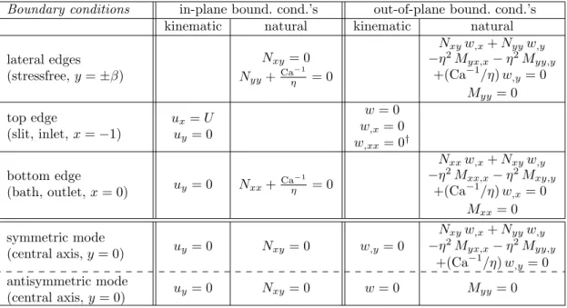
0.08 0.06 0.04 0.02 0.05 0.04 0.03 0.02 0.01 -0.2 -0.4 -0.6 -0.8 -1 -0.2 -0.4 -0.6 -0.8 0.2 0.4 0.8 1.2 2.0 4.0 -1
(a)
(b)
Eq. (22)bath
Figure 2: Retraction of the lateral free edge, based on the numerical solution for the base flow in the absence of surface tension. (a) Profile of the edge (x) as a function of aspect-ratio, based on equation (20). The retraction is exaggerated: the actual one is given by Je (x) with Je⌧ 1. By Stokes-Rayleigh analogy, this retraction is similar to Poisson’s e↵ect in an elastic band. The retraction is more pronounced for wider curtains (i.e. for larger values of ). (b) Retraction scaled by aspect ratio : for small , the retraction is well approximated by the simple model of equation (22), shown by a dashed line.
3.3. Features of the planar solution
Je↵reys’ number Je has been scaled out from the equations for the base flow established in§3.2, and the only parameter left is the half aspect-ratio : the numerical calculation of the base solution yields a family of base flows u(0)↵ ( , x, y) indexed by . The dependence of u(0)↵ on will be implicit from now on.
The shape of the free edge can then be reconstructed as follows. In our rescaled units, the descent velocity is U = 1, up to terms of order Je ⌧ 1. The position of a particle on the lateral edge on the right-hand side is ( 1, ) when it exits from the slit. After a time interval ⌧ , its vertical coordinate is x = 1 + ⌧ and its horizontal velocity is u(0)y ( 1 + ⌧, ) = Je u(0)y ( 1 + ⌧, ). Therefore, the equation for the free edge
reads6, at dominant order in Je, y
fe(x) = + JeR x
1u (0)
y (x0, ) dx0 = Je (x) where (x) denotes the
dimensionless retraction of the free edge, (x) =
Z x 1
u(0)y (x0, ) dx0. (20)
Based on this formula and on the numerical solution for u(0)↵ , the shape of the free edge is shown in figure 2
for various aspect-ratios .
Before we proceed to calculate the stress in the base solution, we come back to the expression of the in-plane strain rate which we obtained in equation (11a) based on a ‘na¨ıve’ rescaling of the in-plane velocities by U , and of the in-plane lengths by H. The expression we obtained was d↵ = u(↵, )+ ⌘2 w,(↵w, )t+· · · .
We can now explain the apparent asymptotic discrepancy in the orders of magnitude of the various terms. In view of equation (17a), the velocity u↵ is of order 1 (i.e. of order U in physical units) but the dominant
contribution is a rigid-body motion, so the velocity gradients are much smaller, of order Je⌧ 1 (i.e. of order Je U/H in physical units). This means that the first term u(↵, )⇠ Je in the right-hand side of equation (11a)
can actually be balanced with the other terms, which are of order ⌘2, provided Je
⇠ ⌘2. We will indeed
adopt this scaling assumption Je⇠ ⌘2later in the analysis of the buckling modes, see
§4. Let us now proceed to plot the rescaled membrane stress N(0)↵ = N
(0)
↵ /Je which, like u(0)↵(x, y) depends
only on (x, y) and . We are particularly interested in negative eigenvalues of N↵ , which correspond to
6Recall that we are working in dimensionless units where in-plane lengths have been rescaled by H and velocities by U ,
injection
bath
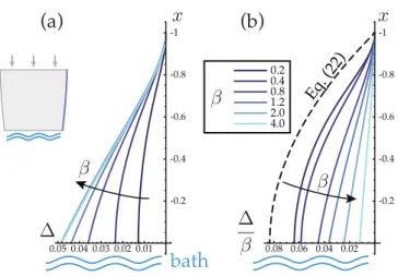
Figure 3: Contour map of the most negative eigenvalue, N(0)I , of the scaled membrane stress N (0)
↵ = N↵(0)/Je in the base
solution for di↵erent aspect-ratios ; surface tension is zero. In blue regions the base flow is tensile in all directions (N(0)I > 0); in red regions, some directions are compressive (N(0)I < 0). In the third map ( = 0.8), the directions of the principal stresses
are shown with arrows: the largest eigenvalue is almost vertical (along x) and the smallest (or most negative) eigenvalue is almost horizontal (along y); blue and yellow arrows correspond to a positive (tensile) and negative (compressive) principal stress, respectively. The orientation of the principal stress directions is similar for all the values of (arrows shown for = 0.8). The small retraction of the free edge is not shown here, see figure 2. Note that the color scale (see legend) is designed to enhance the changes of sign of N(0)I —in spite of the large contrast, the amplitude of oscillations of N(0)I with x in the first figure = 0.2 are small.
directions of compression: in the presence of a negative principal stress, N(0)I < 0 (red regions in figure 3),
a buckling instability is possible if the thickness is small enough. The viscous sheet is stretched vertically but compressed horizontally in the red regions (N(0)I < 0). By contrast, it stretches both in the horizontal
and vertical directions in the blue regions (N(0)I > 0). We observe that, everywhere along the sheet, the
principal stress directions remain almost aligned with the x and y axis (arrows shown for = 0.8 in the figure, but not shown for other values of ). This will be explained based on a simplified one-dimensional model for the flow, see§3.4 below.
The stress maps reveal a strong dependence on the aspect-ratio . In the range 0.4 1.2, there is a single region of compression at the bottom of the sheet near the bath. For smaller values of , this compressive region moves upstream and progressively invades the domain. For = 0.2, it is made up of two components: a small region near the bottom, and a large region in the middle of the sheet — this corresponds to a transverse stress Nyy which is oscillatory with x along the central axis. For larger aspect-ratio, 4,
the flow is tensile almost everywhere, except in the vicinity of the lower corners where the free lateral sides meet with the bath. This stress distribution is similar to that obtained for stretched elastic plates by Friedl et al. (2000), a problem which has been further studied by Cerda et al. (2002); Zheng (2009); Puntel et al. (2011); Healey et al. (2013). It is also similar to that obtained by Filippov and Zheng (2010) using a viscous membrane model (with the added simplification that the motion is close to a rigid translation and that the variation of thickness can be neglected here). The alternation of tensile and compressive regions, the genuine 2D character of the flow, and the sensitivity of the stress distribution to the single geometrical parameter make this system a perfect one for analyzing the stability of viscous sheets. This is the goal we pursue in §4.
3.4. A simple approximation for the base flow
In this section, we propose a simple approximation for the base flow which captures the retraction of the lateral edges shown in figure 2. We do not claim that this approximation is exact in any asymptotic sense.
It is only intended to provide a simple picture of the actual solution. This section is independent of the rest of the paper and can be skipped.
Inspired by the one-dimensional example of a bar hanging under its own weight, we assume a membrane stress N(0)⇡ Je x ex⌦ ex, which satisfies the equilibrium in the interior (15a–15b). Inverting the
constitu-tive law for membrane stress (9a), we obtain the membrane strain rate as d(0) ⇡ Jex
3 ex⌦ ex 12ey⌦ ey ,
or d(0) ⇡ x
3 ex⌦ ex 12ey⌦ ey in dimensionless form. Here, the coefficient 1/2 accounts for Poisson’s
e↵ect. This is only an approximation of the exact solution as we have ignored both some of the boundary condition, and the condition that the strain rate is geometrically compatible—it is not, as evident from the fact that d(0)yy depends on x, although the shear component d
(0)
xx is zero. The vertical component d (0)
xx = x/3
can be integrated into a vertical velocity u(0)x (x, y)⇡ Je(x
2
6 + f (y)) where the constant of integration f is
set by the condition ux= 0 at the top boundary as
u(0)x (x, y)⇡
1 x2
6 . (21a)
Integrating now d(0)yy, we obtain u (0)
y =x y6 + g(x). The symmetry condition yields the constant of integration
as g(x) = 0,
u(0)y (x, y)⇡
x y
6 . (21b)
By comparing to the numerical solution of §3.2–3.3, we have checked that equations (21) are a reasonable approximation of the base flow, especially for wide curtains (large ).
This approximation predicts a retraction of the lateral edge ⇡ Z x 1 ¯ u(0) y y= dx0= Z x 1 ✓ x0 6 ◆ dx0 = 12(1 x 2), (22)
which is in reasonable agreement with the exact solution, as shown as a dashed curve in figure 2b.
In this approximation, one principal stress is tensile and in the vertical direction, N(0)xx = x/3 =
|x|/3 0, and the other one is neutral and in the horizontal direction, N(0)yy = 0. This is consistent
with the numerical finding that the principal stress directions remain everywhere close to horizontal and vertical, see the light blue and yellow arrows in figure 3. However, the approximation cannot predict the sign of the most compressive eigenvalue of the stress N(0)I , which is crucial for the stability analysis. Still, it
explains why N(0)I takes on numerically small values, especially for small , see the stress maps in figure 3.
This introduces numbers in the problem whose absolute values are much less than 1 even though they are mathematically of order 1, i.e. they do not tend to zero in any asymptotic limit. Such small values of N(0)I
are responsible for the numerically small values appearing in the vertical axes of the rescaled phase diagrams, see later in figures 5 and 8.
4. Linear stability analysis: curtain modes
In this section, we analyze the stability of the planar solutions derived in the previous section with respect to out-of-plane perturbations. By means of a finite element discretization, the buckling analysis is formulated as a generalized matrix eigenvalue problem. Due to the presence of advection, the buckling analysis di↵ers significantly from that of an elastic plate, and it involves a non-Hermitian problem.
4.1. Linearized equations for thin sheets
We perturb the base flow with a small time-dependent deflection w(1)(x, y, t):
u↵(x, y, t) = u(0)↵ (x, y) + 0 + · · · (23a)
where(0) denotes the base solution, and(1) the first order perturbation. We may seek a purely transverse
perturbation to first order, see equation above, as the base solution is invariant by reflection with respect to the (xy) plane.
From equations (13–14), the linearized principle of virtual work reads 8 ˆw k.a., ZZ Dt ⇣ Je N(0)↵ ˆ✏ (1) ↵ ⌘ 2M(1) ↵ wˆ,↵ ⌘ dx dy = 0. (24) In equation (24), ˆ✏(1)↵ = w (1)
,↵wˆ, is obtained by linearization of equation (13c) with respect to the real,
incremental deflection. The out-of-plane perturbation does not change the membrane strain rate to first order, d(1)↵ = 0, so N
(1)
↵ = 0 by the constitutive law as well: this is why the term
RR N↵(1)ˆ✏
(0)
↵ dx dy = 0 is
absent from equation (24).
Rewriting the constitutive law (12b) as M↵ = L↵ ⌧k ⌧ with
L↵ ⌧ =
1
6( ↵ ⌧+ ↵ ⌧), (25) and noting that k↵(1) = w(1),↵ t+ u(0)w,↵(1) = w(1),↵ t+ U w,↵ x(1) (up to small corrections of order Je), with U = 1 in our rescaled variables, this becomes
ZZ Dt ⇣ Je N(0)↵ w,↵(1)wˆ, ⌘2L↵ ⌧ h w, ⌧ t(1) + w(1), ⌧ x i ˆ w,↵ ⌘ dx dy = 0.
The square bracket contains the linearized version of the bending strain rate k: the last (co-rotational) term present in the general definition (8b) of k has disappeared and it plays no role in the particular problem studied here.
Since the base flow is stationary, we seek modes w(1)(x, y, t) having an exponential dependence on time,
w(1)(x, y, t) = W (x, y) e i ! t, (26) where the angular velocity ! is a complex eigenvalue. The weak form of the equations for the linear modes becomes ZZ Dt ✓ N(0)↵ W,↵wˆ, ⌘2 JeL↵ ⌧W, ⌧ xwˆ,↵ ◆ dx dy = i! ⌘ 2 Je ZZ Dt L↵ ⌧W, ⌧wˆ,↵ dx dy (27)
In terms of the pre-stress distribution N(0)↵ (x, y) available from §3.3, this equation defines an eigenvalue
problem for W (x, y) and !, which we now solve numerically. This type of eigenvalue problem arises generally in the stability analysis of rate-independent systems, see for instance Triantafyllidis and Leroy (1994). 4.2. Discretization of the buckling problem
One may notice that the weak form of the out-of-plane problem involves third order derivatives, which are due to advection terms. These terms give rise to fifth order derivatives in the strong form of the balance of stress, meaning that high-order elements are required in the finite-element method. C1-type finite elements
have been designed for plate-like problem, and can be applied directly to variational problems involving second order derivatives in both the test and trial functions (hence to problems involving into fourth-order derivatives in strong form). In our problem, an additional, third-order derivative of the test function is present. We take care of it using a classical method, described for instance by Xu and Shu (2008). The main idea is to use a redundant unknown ⇥(x, y) to represent the gradient W,x(x, y) of the deflection unknown
W : the original third-order derivative W, ⌧ x are then available as the second-order derivative of the new
variable ⇥. This e↵ectively decreases the order of derivation to two in the weak formulation, so that standard C1-smooth elements can be used. This comes at the price of adding a new variable. A constraint must be set
up, so that the new variables ⇥ matches W,x, as intended. This constraint is handled in our implementation
We define a new complex unknown field ⇥(x, y) representing the slope W,x(x, y). The modified variational
formulation is as follows: one seeks the complex fields W (x, y) and ⇥(x, y) and the complex eigenvalue ! such that, for any virtual displacement ( ˆw, ˆ✓) satisfying the incremental kinematic boundary conditions, ZZ Dt ✓ N(0)↵ W,↵wˆ, ⌘2 JeL↵ ⌧⇥, ⌧wˆ,↵ ⇤ (⇥ W,x) ˆ✓ ◆ dx dy = i! ⌘ 2 Je ZZ Dt L↵ ⌧W, ⌧wˆ,↵ dx dy. (28) An additional penalty term has added to the weak form (27). The penalty parameter ⇤ is chosen large enough for the equality ⇥ = W,x to be satisfied to a prescribed accuracy.
The eigenvalue problem (28) concerns a dissipative system and is not Hermitian, as can be checked directly.
4.3. Numerical eigenvalue analysis
In equation (28), the unknowns are the spatial part (W, ⇥) of the eigenmodes, and the eigenvalue is the complex frequency ! or, equivalently, the stability exponent ( i !). We proceed to discretize this problem using the finite element method. The variables W and ⇥ are discretized using C1elements to comply with the
presence of second-order spatial derivatives in equation (28). Specifically, we use a Hermite polynomials basis with Bogner-Fox-Schmidt element types, a popular choice for elastic plate problems Rustein (2008). We use the open source C++ finite elements library libmesh, leveraging the powerful numerical tools PETSC (Balay et al., 1997, 2014b,a) for matrix algebra and SLEPC (Hernandez et al., 2005) for eigenvalue analysis. Upon discretization of equation (28), we obtain a generalized matrix eigenvalue problem in the form
[ ˆw, ˆ✓]· A ✓ ,⌘ 2 Je ◆ · [W, ⇥] = i! ⌘ 2 Je [ ˆw]· B · [W ], (29) where the assembly of the matrices A and B is described below, and the eigenvalue! ⌘Je2 is the scaled complex frequency. The matrix A is assembled from all the terms in the variational form (28) that include no time derivative; by contrast, the matrix B gathers all the terms involving a time derivative—all of which come from viscous bending. As the term N(0)↵ W,↵wˆ, in equation (28) is taken care of by A, the pre-stress
N(0)↵ must be determined prior to assembling A; this is why A depends on the aspect-ratio . A depends
on the parameter ⌘2/Je as well because of the second term in the integrand in the left-hand side of (28).
This parameter enters as a multiplicative coefficient in the right-hand side of (28) and has been factored out from B.
The step following the assembly of the matrices A and B is to solve the discrete eigenvalue problem (29). We are specifically interested in finding the vector (W, ⇥) associated with the largest real growth rate (Im !) as this is the most unstable mode. This corresponds to finding the eigenvalue i!⌘2/Je with the smallest
real part. For maximal efficiency, we use a solver based on an iterative Krylov-Schur method combined with a spectral transformation method (shift-and-invert), which can return a few eigenvectors corresponding to the largest growth rates. Some of the eigenmodes are jagged, i.e. undulating with a length scale comparable to the mesh size (grid modes), and are discarded. Typical eigenvectors corresponding to the largest growth rate are shown in figure 4 for di↵erent values of , and for values of ⌘Je2 close to the onset of the instability.
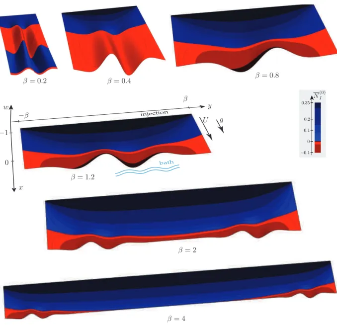
One can notice that the eigenmodes are mostly concentrated in the regions where the base flow is compressive (red regions in figure 3 and 4), as expected. As apparent from the plot for = 0.2, the eigenmodes decay along the direction the flow (downwards) in the regions where the pre-stress N(0)↵ is
tensile in all directions, hence locally stable (blue regions). The modes are undulating in the transverse direction y, much like a hanging curtain: this is because a negative principal stress in the base solution always takes place in a nearly transverse direction, see the yellow arrows in figure 3.
The wavelength of the curtain is significantly smaller than the size of the system. This contrasts with buckling problems involving a homogeneous base solution, where the wavelength is usually set by the size the system. Indeed, for the viscous curtain, the base flow is far from homogeneous for the problem. As a
Figure 4: Shape of the most unstable buckling mode for di↵erent aspect ratios , without surface tension. For every value of , a di↵erent value of the parameter⌘Je2 is picked such that the sheet is close to the limit of stability: the di↵erent plots correspond to , log10⌘
2
Je = 0.2, 6.9 , 0.4, 5.8 , 0.8, 4.5 , 1.2, 4.5 , 2, 4.9 and 4, 5.0 , respectively, as indicated by a star
in the phase diagram in figure 5. The four modes with 1.2 are not oscillatory (Re ! = 0), while the two ones with 2 are oscillatory (Re !6= 0). The colors encode the most negative eigenvalue of the stress in the base flow, as in figure 3: the instability develops in compressive regions, shown in red.
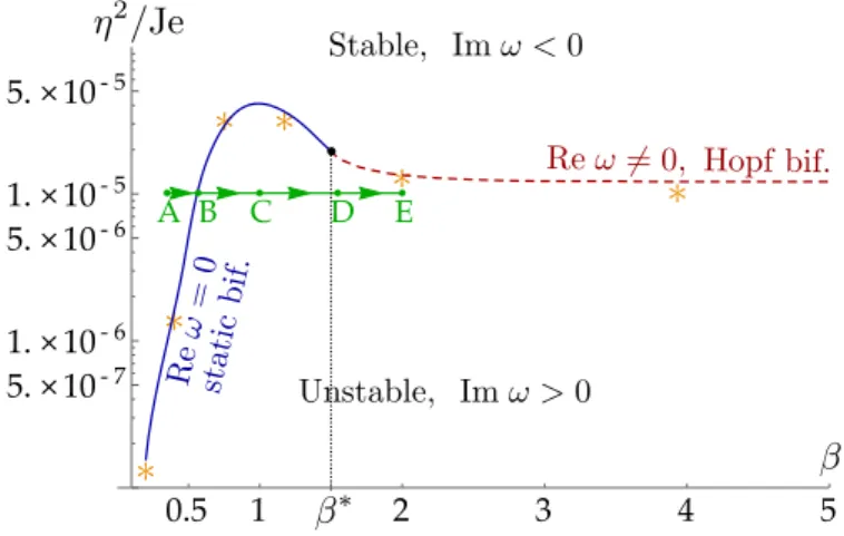
A B C D E 0.5 1 2 3 4 5 5. × 10- 7 1. × 10- 6 5. × 10- 6 1. × 10- 5 5. × 10- 5
Figure 5: Phase diagram without surface tension: critical scaled thickness squared, ⌘Je2, as a function of the aspect-ratio . The curves of marginal stability are obtained as the locus of Im ! = 0, where ! is the complex frequency of the most unstable eigenmode. The dashed curve corresponds to an oscillatory mode (Re !6= 0) obtained by a Hopf bifurcation, and the solid curve corresponds a non-oscillatory, buckling mode (Re ! = 0) obtained by a static bifurcation. The green path going from A to E is used to track the bifurcation from a static to an oscillatory mode, as studied in detail in figure 6; ⇤is the critical value of aspect ratio where oscillatory modes appear. The star symbols refer to the eigenmodes shown in figure 4. The numerical values on the vertical axis of this phase diagram are small because the base flow is only mildly compressive, even in rescaled variables, as noted at the end of§3.4.
result, the wavelength of the instability is essentially set by the length scale at which the stress varies in the base solution, rather than by the size of the system. The eigenmodes are reminiscent of those obtained for elastic plates in the work of Friedl et al. (2000); Kim et al. (2012); Nayyar et al. (2011); Zheng (2009); Puntel et al. (2011); Fischer et al. (2000). Note that the present system is non-conservative, because of viscosity and of the open character of the flow: as a result, oscillatory linear modes are possible (Im ! = 0 and Re !6= 0)—the modes = 2 and = 4 shown in figure 4 are indeed oscillatory, as discussed below. For those oscillatory modes, the plots in figure 4 are based on the real part of the eigenmodes and the imaginary part is not shown.
4.4. Phase diagram
In this linear analysis, an instability takes place when the growth rate (Im !) of the eigenmodes shown in figure 4 becomes positive. This happens when the sheet is thin enough, i.e. when the dimensionless thickness ⌘ is small enough. More accurately, the stability of the planar configuration is determined by the scaled thickness squared ⌘2/Je and by the aspect ratio , see equation (29). By analyzing the sign of the
largest growth rate Im ! as a function of these parameters, a phase diagram can therefore be plotted in the ( ,⌘Je2) plane, see figure 5. According to this phase diagram, the linear stability depends on the parameter
⌘2
Je = µ U h2
⇢ g H4: the planar flow is linearly stable above a critical value of this parameter depending solely on
the aspect-ratio , and linearly unstable below. In terms of the physical parameters, the flow is therefore stable when the thickness h is above a critical value depending on the physical parameters of the problem, and unstable below, as usual in plate buckling instabilities: increasing the thickness corresponds to moving upwards in the phase diagram.
When the flow is marginally stable (Im ! = 0), the mode can either be static (Re ! = 0) or oscillatory (Re ! 6= 0), corresponding to the solid and dashed curves in figure 5, respectively. A static bifurcation is obtained for small aspect-ratios < ⇤ and an oscillatory (flutter-like, or Hopf) bifurcation is obtained for
larger aspect-ratios, > ⇤. The change in behavior occurs for ⇤= 1.5 (this number depends only on the
boundary conditions). Note that the presence of oscillatory modes is made possible by the non-Hermitian character of the eigenvalue problem, as a consequence of both viscous dissipation and of the open flow.
A B C D E E -0.3 -0.2 -0.1 0.1 0.2 0.3 -5 5 10 15 Stable Unstable static Hopf Hopf
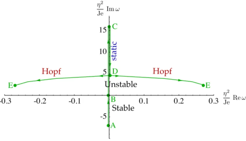
Figure 6: Analysis of the transition from static to oscillatory modes: motion of the growth rate ! in the complex plane when the aspect ratio is varied, for fixed ⌘2/Je = 10 5. The curves are the paths traced out by ! as the aspect ratio is varied
from = 0.4 to = 2, corresponding to the path joining the points labelled A and E in figure 5. Point B corresponds to the value of the aspect ratio at which the system becomes unstable, i.e. where the green line in figure 5 intersects the curve of marginal stability. At point C the system has the largest possible growth rate for this particular choice of parameters. At point D the instability becomes oscillatory, as the double eigenvalue ! splits into a pair of eigenvalues having opposite real parts.
Triantafyllidis and Leroy (1994) studied a stability problem involving viscous and elasto-plastic dissipation but no open flow, and found only static bifurcations.
To analyze the transition from static to oscillatory modes, we consider the path A!E traced out in the phase diagram in figure 5, and track the corresponding motion of the most unstable eigenvalues ! in the complex plane, see figure 6. At point A, the eigenvalues are located in the stable half-plane Im ! < 0. At point B, when the path crosses the curve of neutral stability, the mode becomes marginally stable, Im ! = 0; the bifurcation is then static, so ! = 0, see figure 6. Further along the path, ! becomes real and positive (unstable mode obtained by a static bifurcation), reaches a maximum at C which is roughly where the path enters most deeply into the unstable region, and then decreases up to point D where the double real eigenvalue splits into a pair of conjugate complex eigenvalues. The corresponding modes remain unstable all the way to the end E of the path. This shows that the oscillatory mode is produced by a continuous bifurcation from the static mode: the angular frequency of the oscillatory mode| Re !| varies smoothly from zero when is increased beyond ⇤.
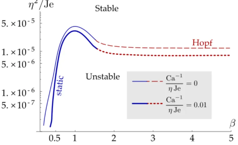
5. E↵ect of surface tension 5.1. Restoring surface tension
We have included the surface tension in our derivation of the governing equations (§2) but have ignored it since then by setting Ca 1= 0 at the beginning of§3. Here, we extend the analysis of the base flow of §3 and the linear stability analysis of§4 to restore the e↵ect of surface tension,
Ca 1> 0. (30)
As we shall show, a moderate change in surface tension modifies quantitatively the base flow and its stability, but not qualitatively.
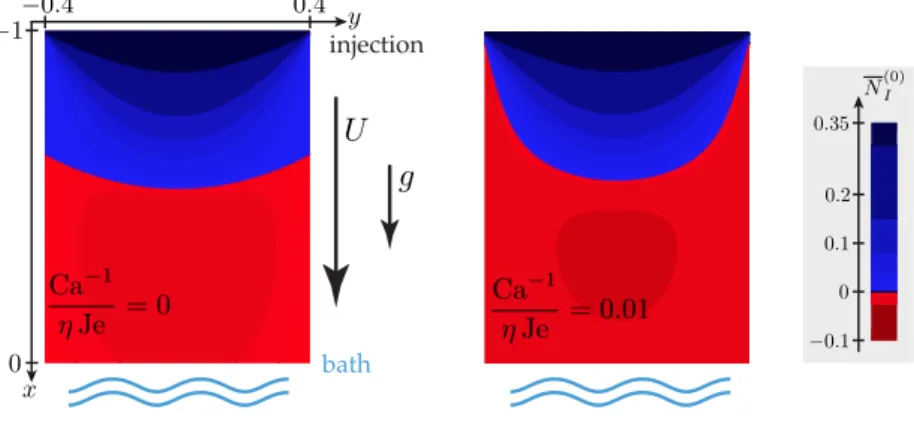
Surface tension tends to minimize the area of the fluid-air interface, which for a thin plate is twice the area of the midsurface, see equation (10c). It a↵ects the stability of the film in two antagonistic ways. On one hand it enhances the contraction of the lateral edges of the curtain and as a result tends to make the horizontal stress Nyy(0) more compressive, and the base flow more unstable (compare the upper halves of the