HAL Id: hal-01668425
https://hal.archives-ouvertes.fr/hal-01668425
Submitted on 15 Mar 2018
HAL is a multi-disciplinary open access archive for the deposit and dissemination of sci-entific research documents, whether they are pub-lished or not. The documents may come from teaching and research institutions in France or abroad, or from public or private research centers.
L’archive ouverte pluridisciplinaire HAL, est destinée au dépôt et à la diffusion de documents scientifiques de niveau recherche, publiés ou non, émanant des établissements d’enseignement et de recherche français ou étrangers, des laboratoires publics ou privés.
Enhanced density-based models for solid compound
solubilities in supercritical carbon dioxide with
cosolvents
Martial Sauceau, Jean-jacques Letourneau, Dominique Richon, Jacques Fages
To cite this version:
Martial Sauceau, Jean-jacques Letourneau, Dominique Richon, Jacques Fages. Enhanced density-based models for solid compound solubilities in supercritical carbon dioxide with cosolvents. Fluid Phase Equilibria, Elsevier, 2003, 208 (1-2), pp.99-113. �10.1016/S0378-3812(03)00005-0�. �hal-01668425�
Enhanced density-based models for solid compound solubilities
in supercritical carbon dioxide with cosolvents
M. Sauceau
a, J.-J. Letourneau
a, D. Richon
b, J. Fages
a,∗aLaboratoire de Génie des Procédés des Solides Divisés, UMR CNRS 2392,
École des Mines d’Albi-Carmaux, Albi 81013, France
bLaboratoire de Thermodynamique des Équilibres entre Phases/CENERG,
École des Mines de Paris, Fontainebleau 77305, France
Abstract
The ability to correlate and predict the solubility of solids in supercritical fluids is of the utmost importance for the design and the evaluation of supercritical processes. Previously, we have investigated the solubility of a pharmaceutically interesting solid compound in supercritical carbon dioxide, alone or mixed with cosolvents. In this work, these solubility data are correlated through several density-based semi-empirical models. These models have been either modified or extended to be applied to mixtures including a cosolvent. The validity of the resulting correlations is checked by using the solubility data of another pharmaceutical solid, naproxen.
Keywords: Solid-fluid equilibria; Solubility; Supercritical carbon dioxide; Cosolvent; Modeling
1. Introduction
Supercritical fluids (SCF) are widely used in many fields of application. The interest in using this technology is due to the special properties that are inherent to this class of fluids. This includes the ability to vary easily and over a large extent the solvent density, and to effect a drastic change in solvent properties by changing either the pressure or the temperature. The most common SCF, carbon dioxide (CO2), is easy to handle, inert, nontoxic, nonflammable, and has convenient critical coordinates. The applications often involve solutes that are in solid state at conditions where the solvent is in supercritical conditions. Thus, the knowledge of the solubility of solids in involved supercritical fluids is essential for evaluating the feasibility and for establishing optimum operating conditions.
∗ Corresponding author. Tel.:+33-5-6349-3141; fax: +33-5-6349-3025.
Table 1
Experimental data for PC in supercritical CO2
Cosolvent Cosolvent mole fraction y3(%) Pressure P (MPa) Temperature T (K) Number of data
None – 9.9–29.70 308.15 9 None – 9.3–30.2 318.15 11 Ethanol 5 9.8–30.4 318.15 11 Ethanol 4.0–17.1 20 318.15 6 DMSO 2 12.2–29.1 318.15 6 DMSO 0.9–3.3 20 318.15 7
All the data from[1].
Because of the limited amount of experimental data dealing with solid-SCF systems, there is consid-erable interest in mathematical models that can accurately predict the phase behavior of such systems. Some of the commonly used models that have been used with some success to correlate solid solubility data include equations of state (EoS). However, such models often require properties (such as critical temperature, critical pressure and acentric factor) that are not available for most of solid solutes. Also, the models require one or more temperature-dependent parameters, which must be obtained from solid solubility data in pure fluids. For these reasons, EoS based models cannot be easily used to predict solu-bilities. Several authors have noticed that the logarithm of solid compound solubilities is approximately a linear function of the SCF density. This observation allows the representation of the solubility by using semi-empirical models, based on density instead of pressure. These relations are very useful because the knowledge of the above mentioned physical properties is not necessary.
In a previous paper, the solubility of a pharmaceutical compound, called PC, was investigated[1]by means of an apparatus based on an open circuit method[2]. The solubility was measured in pure supercrit-ical CO2and in supercritical CO2mixtures with ethanol and dimethylsulfoxide (DMSO) (Table 1). In this work, these experimental equilibrium solubilities are correlated using three different models, developed and extended to be applicable to solvent–cosolvent mixtures.
2. Data correlation
The first model was proposed by Chrastil[3]. This may be considered as a macroscopic description of the surroundings of the molecules in the fluid phase. It is based on the hypothesis that one molecule of a solute A associates with k molecules of a solvent B to form one molecule of a solvato-complex ABk in equilibrium with the system. The definition of the equilibrium constant through thermodynamic considerations leads to the following expression for the solubility:
ln(C2)= k ln(ρf)+ α
T + β (1)
where C2 is the concentration of the solute in the supercritical phase, ρf the density of the fluid phase,
k the association number, α depends on the heat of solvation and the heat of vaporization of the solute
and β depends on the molecular weight of the species. Parameters k, α and β are adjusted to solubility experimental data.
The second model was developed by Ziger and Eckert[4], partly on the basis of the regular solution theory and the van der Waals equation of state (vdW EoS). In this treatment, the vdW EoS and mixing
rules are used to evaluate the fugacity coefficient of the solute in the SCF phase in terms of solubility parameters of the solute and the solvent. The Hildebrand solubility parameter, δ, is an indicator of the strength of intermolecular forces present in a solute or solvent and is defined as the square root of the cohesive energy density. The final expression for the semi-empirical correlation derived by Ziger and Eckert[4]is represented by the following equation:
log10E = η1 ! ε2 ∆ y1 " 2− ∆ y1 # − log10 " 1+" δ1 2 P ##$ + ν1 (2) where E = y2P P2sat, ε2 = (δ2)2vL2 2.3RT and ∆ = δ1 δ2 (3)
where yi is the equilibrium mole fraction of the compound i in the SCF phase, P the total pressure, P2sat the sublimation pressure of the solute, δi the solubility parameter of the compound i, R the ideal gas constant and v2L the molar volume of the solute in liquid state. E is the enhancement factor defined as the ratio between the observed equilibrium solubility and that predicted by the ideal gas law at the same temperature and pressure, ε2represents a dimensionless energy parameter and ∆ is the ratio of solubility parameters for solvent and solute. Parameters η1and ν1represent constants obtained by regression of the experimental data that are characteristics of each solvent and solute, respectively.
The third model is based on the theory of dilute solutions, which leads to simple expressions for many thermodynamic properties of dilute near-critical binary mixtures. In particular, Harvey[5]has obtained a simple linear relationship for the solubility of a solid in a supercritical solvent. Mendez-Santiago and Teja[6]have approximated this relationship by
T ln E = A1+ B1ρf (4)
where A1 and B1 are adjustable parameters. They have also incorporated a Clausius–Clapeyron type equation for the sublimation pressure and obtained a new correlation with three adjustable parameters A′1, B1′ and C1′ [6]:
T ln y2P = A′1+ B1′ρf + C1′T . (5) However, the Clausius–Clapeyron equation could be advantageously written with the dimensionless logarithm: lnP sat 2 Pstd = i − j T (6)
where Pstd is the standard pressure (atmospheric pressure equal to 0.101325 MPa). This provides the following correlation with three adjustable parameters A2, B2and C2:
T ln y2P
Pstd = A2+ B2ρf + C2T . (7)
Finally, in another paper, the same authors [7] have improved the Eq. (4) by taking into account the cosolvent mole fraction, y3:
T ln E = A3+ B3ρf + D3y3 (8)
3. Results and discussion
3.1. Density calculations
The three correlations require the knowledge of supercritical mixture densities. As the pharmaceutical compound solubility is extremely low, the density change due to the presence of the solid compound is negligible and then it is neglected. As a consequence, the density of the saturated supercritical phase is taken equal to the density of the solvent (CO2 or CO2+ cosolvent). The pure CO2 density is calculated by using the Peng–Robinson equation of state[8](PR EoS). For the mixtures involving a cosolvent, the density is calculated by using the PR EoS[8], with two quadratic mixing rules and two binary interaction parameters, kij and lij (Table 2), from works of Kordikowski et al.[9]and of Ting et al.[10].
The quality of all data correlations is quantified by the average absolute deviation (AAD), defined as follows: AAD= 1 n n % i=1 & & & & y2,cal− y2,exp y2,exp & & & & i × 100 (9)
where n is the number of data, y2,cal the calculated solubility value and y2,expthe experimental one.
3.2. Extension of the Chrastil model
The Eq. (1) is first applied to solubility data of the pharmaceutical solid PC in pure CO2. The two isotherms are well fitted (lines 1 and 2 ofTable 3), the AAD being less than 8%. The k value obtained shows small temperature dependence. If the data of the two isotherms are gathered before parameter adjustment, the AAD remains practically constant (line 3).
The Chrastil model is applicable to pure fluids. Thus, we could apply it to mixtures at constant cosolvent mole fractions, with the hypothesis that these mixtures at constant concentration behave like pure fluids. The results are listed inTable 3(lines 4 and 5). The data are well correlated with an AAD less than 6%. The same treatment can be made as for the Chrastil model, with the assumption that one molecule of a solute A associates with k1 molecules of a solvent B and k3 molecules of a cosolvent C to form one molecule of a solvato-complex ABk1Ck3. Finally, theEq. (1)becomes:
ln(C2)= (k1+ k3)ln(ρf)+ α
T + β. (10)
Table 2
Cosolvent critical properties and binary interaction parameters with CO2
Cosolvent TC(K) PC(MPa) ω kij lij DMSOa 720.0 5.705 0.350 0.015 −0.025 Ethanola 516.2 6.384 0.635 0.089 0.000 Ethyl acetatea 523.0 3.83 0.362 −0.02 0.010 Acetoneb 508.2 4.66 0.318 0.0137 0.000 Methanolb 512.6 8.09 0.556 0.0749 0.000 aData from[9]. bData from[10].
Table 3
Correlation of PC solubility data withEq. (1)
Cosolvent T (K) Data Eq. (1)
k α(×103K) β AAD (%)a None 308.15 9 7.11 −6.92 −31.26 6.2 None 318.15 11 6.44 −7.97 −23.06 7.1 None All 20 6.55 −10.89 −14.62 7.7 Ethanol: 5% 318.15 11 7.18 −28.92 −39.53 5.9 DMSO: 2% 318.15 6 10.13 −7.24 −47.34 4.7 aDefined inEq. (9).
The values of k obtained inTable 3are thus the number of molecules of solvent k1 and cosolvent k3 associated with one molecule of solute. These numbers are higher than that in pure CO2: 7.2 with 5% of ethanol and 10.1 with 2% of DMSO instead of 6.5 in pure CO2. This confirms the importance of specific interactions in the solubility enhancement phenomenon[1].
3.3. New correlation using a modified Ziger and Eckert model
Applying the Ziger and Eckert model requires the estimation of the thermodynamic properties of pure components, for both the solvent and the solute. As noted by Giddings et al. according to the vdW theory
[11], the solubility parameter of the pure SCF can be written as follows:
δ1 = (a1) 1/2ρ
1 M1
(11)
where M1 is the solvent molecular weight and a1 the energy parameter of the solvent in vdW equation, calculated by
a1 = 27 64
R2TC2
PC . (12)
Ziger and Eckert [4] consider the solid solute as a subcooled liquid and hence evaluate all the solute parameters after extrapolation of liquid properties from the melting point using a thermal coefficient. Gurdial and Foster[12]suggested that thermodynamic properties could be estimated more readily from an atomic and group contribution method as proposed by Fedors[13]. This atomic and group contribution method, which requires only the knowledge of the structural formula of the compound, is applicable not only to linear compounds but also to organometallic and cyclic compounds at 298.15 K. In the case of a cyclic compound, this is accomplished by adding cyclization increments to both the energy of vaporization and the molar volume of a linear compound having the same chemical structure as the cyclic compound of interest. Fedors[13]has also proposed relationships to take into account the temperature influence on both the molar volume and the solubility parameter for low temperature variations (<50 K). This approach was adopted for the evaluation of the solubility parameter and molar volume of our solid compound. However, due to the lack of experimental data, the thermal expansion coefficient for our solute was assumed to be similar to the value for naphthalene (0.0007 K−1)[12]. The values obtained are listed inTable 4.
Table 4
Estimation of solubility parameters and molar volumes of solids compounds Compound
PC Naproxen
298.15 K 308.15 K 318.15 K 313.1 K 323.1 K 323.1 K ν2L(cm3mol−1)a 414.2 417.1 420.0 177.9 179.2 180.4
δ2(MPa1/2)a 22.5 22.3 22.2 23.4 23.2 23.1
aEstimated by the method proposed by Fedors[13].
The Ziger and Eckert model requires also the knowledge of the saturated vapor pressure of the solute, P2sat, for calculating the enhancement factor, E. As this pressure is unknown for the solid PC, Psat
2 is replaced by a Clausius–Clapeyron equation, asEq. (6). An improved correlation, with three adjustable parameters η2, κ2 and ν2, is thus obtained:
log10" y2P Pstd # = η2 ! ε2∆ y1 " 2− ∆ y1 # − log10 " 1+" δ 2 1 P ##$ + κ2 T + ν2. (13)
Eq. (13)is valid for pure fluids. Thus, it has been modified to be applicable to cosolvent mixtures with a constant cosolvent mole fraction. The new expression is
log10" y2P Pstd # = η3 ! ε2 ∆ 1− y2 " 2− ∆ 1− y2 # − log10 " 1+" δ 2 m P ##$ + κ3 T + ν3 (14) with δm = (am) 1/2ρ f y1M1+ y3M3 (15)
where δmis the solubility parameter of the solvent–cosolvent mixture. It depends on the mole fraction yi and the molecular weight Miof the pure compound i, and also on the density ρfand the energy parameter in vdW equation amof the solvent–cosolvent mixture. Parameter am is calculated from pure component parameters by using a quadratic mixing rule:
am = % i % i yiyjaij with aij =√aiiajj(1− kij) and aii = ai (16) where kij is a binary interaction parameter, already used before (Table 2). If no cosolvent is used, δm is equal to δ1, its value in pure CO2, andEqs. (13) and (14)are identical. Results for this equation are listed inTable 5. The two isotherms of solubility in pure CO2are well fitted byEq. (14)(lines 1 and 2), the AAD being less than 13%. As for the k value in Chrastil model, the η3value obtained shows small temperature dependence. If the two isotherms are gathered before parameter adjustment, the AAD remains practically constant (line 3). For mixtures with a constant cosolvent mole fraction, a good correlation is obtained with an AAD less than 7% (lines 4 and 5). The parameter η3, characteristic of the solvent[4], is increased in presence of cosolvent: from 0.20 for pure CO2 to 0.24 with a 5% ethanol mole fraction and to 0.31 with a 2% DMSO mole fraction. This confirms that the mixtures at constant concentration behave like pure fluids, with, however, a better solvent power than pure CO2.
Table 5
Correlation of PC solubility data withEq. (14)
Cosolvent T (K) Number of data Eq. (14)
η3 κ3(K) ν3 AAD (%)a None 308.15 9 0.22 −2.06 −3.23 12.6 None 318.15 11 0.19 5.12 −24.65 9.9 None All 20 0.20 −7.36 14.45 11.1 Ethanol: 5% 318.15 11 0.24 −1.06 −5.56 7.1 DMSO: 2% 318.15 6 0.31 −3.65 1.16 4.3 aDefined inEq. (9).
However, this correlation cannot represent the variation of the cosolvent mole fraction. As can be seen on Fig. 1, log10(y2P /Pstd)shows a linear dependence with log10(y3)at a given temperature. This observation leads to adding an additional term inEq. (14), as follows:
log10" y2P Pstd # = η4 ! ε2 ∆ 1− y2 " 2− ∆ 1− y2 # − log10 " 1+" δ 2 m P ##$ + κ4 T + λ4log10y3+ ν4. (17) This new relationship has four adjustable parameters: η4, κ4, λ4 and ν4. As can be seen in the first two lines of Table 6, good results are obtained when applyingEq. (17)to mixtures with ethanol or DMSO. As solubility data with a cosolvent are available at only one temperature, correlation is carried out with the constant relative to temperature, κ4, equal to that obtained for all temperatures in pure supercritical CO2, κ3(third line ofTable 5). This modification involves no change in values of η4and λ4(two last lines in Table 6). As already observed by Ziger and Eckert [4], η4 and ν4 are constants for each solvent and solute, respectively. Thus, η4 is different for each solvent–cosolvent mixture, while ν4remains constant.
Table 6
Correlation of PC solubility data withEq. (17)
Cosolvent Number of data Eq. (17)
η4 κ4(K) λ4 ν4 AAD (%)a Ethanol 17 0.24 −0.63 1.71 −4.71 6.6 DMSO 13 0.31 0.80 2.17 −9.04 9.0 Ethanol 17 0.24 −7.36 1.71 16.43 6.6 DMSO 13 0.31 −7.36 2.17 16.58 9.0 aDefined inEq. (9).
κ4is fixed by pure CO2data and thus is the same for the two cosolvents. The higher increase of cosolvent effect with cosolvent mole fraction for DMSO is expressed by the higher value of λ4.
3.4. Generalizing the Mendez-Santiago and Teja model
Eq. (7) has directly been applied to all data in pure CO2 as it takes into account the temperature. It provides a good correlation, with an AAD about 6% (first line inTable 7).
As already done by Mendez-Santiago and Teja inEq. (5), a Clausius–Clapeyron-type equation (Eq. (6)) is incorporated for the sublimation pressure inEq. (8)to give the new correlation, with four adjustable parameters:
T ln" y2P Pstd
#
= A4+ B4ρf + C4T + D4y3. (18) Results for this correlation are presented inTable 7. In a first attempt, solubility data are treated indepen-dently for each cosolvent, by gathering data at different pressures and cosolvent mole fractions. The two data at higher ethanol mole fractions (16.2 and 17.1%) are ignored because they provoke a large increase in the AAD. Data are well fitted, with an AAD about 6% for ethanol (line 2) and about 19% for DMSO (line 3). AAD for DMSO is larger probably because there are more data at different mole fraction values
Table 7
Correlation of PC solubility data withEqs. (7), (18) and (19) Cosolvent Number of data Eq. (18)
A4(K) B4(K m3kg−1) C4 D4(K) AAD (%)a – 20 −16.24b 3.53c 33.35d – 6.4 Ethanol 15 −6.42 3.84 1.89 8.57 6.4 DMSO 13 −4.61 4.85 −6.26 34.13 19.1 Ethanol 35 −16.63 3.59 34.45 9.40 7.7 DMSO 33 −16.93 3.63 35.30 38.90 14.8 All 48 −17.16e 3.67f 35.96g 9.16h 12.7 38.59I aDefined in Eq. (9).b,c,dcoefficients A
2, B2 and C2, respectively, from Eq. (7); e,f,g,h,icoefficients A5, B5, C5, D5 and E5,
(7 instead of 4). However, data are available at only one temperature, which is not enough to determine correctly the value of the parameter, C4, related to temperature. In order to have data at two different temperatures, a second correlation is carried out by gathering data for each cosolvent with that in pure CO2(lines 4 and 5). Finally, the AAD remains constant at about 8% for ethanol and decreased from 19 to 15% for DMSO, with coefficients attributed to density, B4, and to temperature, C4, close to those obtained in pure CO2. It shows that these two coefficients can be considered to be independent of the presence of a cosolvent. It has also to be noted that the value obtained for the coefficient A4 remains practically constant in CO2 alone and with a cosolvent. The part of cosolvent effect due to specific interactions between solute and cosolvent is thus independent of density and temperature effects, and is quantified by the value of cosolvent mole fraction coefficient, D4. On the basis of these observations, a correlation of all PC solubility data can be carried out by using the following equation with five adjustable parameters:
T ln" y2P Pstd
#
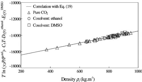
= A5+ B5ρf + C5T + D5y3ethanol+ E5y3DMSO. (19) The data in pure CO2 are treated with: y3ethanol = y3DMSO = 0, and the ones with a cosolvent with: y3DMSO = 0 for ethanol as cosolvent and y3ethanol = 0 for DMSO as cosolvent. All the data are finally correlated with a value of the AAD less than 13% (last line in Table 7). This correlation characterizes the solubility of the solid studied in supercritical CO2 by using only one equation: effects of density, of temperature and of each cosolvent are quantified by means of constant values. As previously noted, the effect due to DMSO (E5 at about 38,600) is higher than that of ethanol (D5 at about 9200). By plotting T ln(y2P /Pstd)− C5T − D5y3ethanol− E5y3DMSOversus ρf, all solubility data are gathered on a single line (Fig. 2).
3.5. Validation with naproxen
In order to expand the validity of the new correlations proposed in this work, they have been applied to the data of another pharmaceutical compound. We have chosen naproxen, because data are available, not only in pure CO2, but also with several cosolvents[10]. The data used in this work are listed inTable 8.
Table 8
Experimental data of naproxen in supercritical CO2
Cosolvent Number of data Pressure P (MPa) Temperature T (K) Cosolvent mole fraction y3(%)
– 18 9–17.9 313.1, 323.1, 333.1 – Ethanol 24 11–17.9 323.1, 333.1 1.75, 3.5, 5.25 Ethyl acetate 18 11–17.9 333.1 1.75, 3.5, 5.25 Acetone 33 11–19.3 313.1, 323.1, 333.1 1.75, 3.5, 5.25 Methanol 26 11–19.3 323.1, 333.1 1.75, 3.5, 5.25 Table 9
Correlation of naproxen solubility data withEq. (17) Cosolvent Number of data Eq. (17)
η4 κ4(K) λ4 ν4 AAD (%)a – 18 0.33b −4.20c – 7.47d 4.2 Ethanol 24 0.33 −4.66 1.23 11.47 2.8 Ethyl acetate 18 0.36 −0.27 0.69 −3.25 3.6 Acetone 33 0.33 −4.10 0.77 8.69 7.2 Methanol 26 0.35 −3.95 1.16 8.94 5.8
aDefined inEq. (9).b,c,dcoefficients η
2, κ2, ν2, respectively, fromEq. (13).
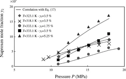
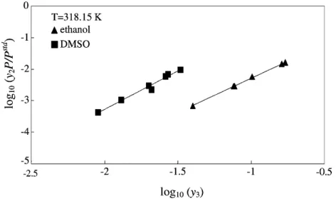
The first model applied is theEq. (17). As for PC, the thermal expansivity of naproxen was assumed to be similar to that of naphthalene. The molar volumes and solubility parameters obtained for naproxen are listed inTable 4. Good correlation of data in pure CO2is obtained with an AAD less than 5%. (first line inTable 9). If a cosolvent is used, an important point for the applicability of Eq. (17)is the isothermal linear dependence of log10(y2P /Pstd)versus log10(y3). This assumption is confirmed for all cosolvents and illustrated onFig. 3in the case of ethanol at 333.1 K. Finally, the application of this relationship to
Fig. 4. Naproxen solubility vs. pressure with acetone as cosolvent: measurements and correlation withEq. (17).
data with a cosolvent gives very good results (lines 2–5 in Table 9). The maximum AAD is 7.2% for acetone for which there is the largest quantity of data, with a good representation of solubility data as shown on Fig. 4. Contrary to what has previously been observed for PC, the parameter η4 is practically constant for all cosolvent–solvent mixtures, at about 0.33, while ν4depends on cosolvent. This value of ν4 allows classifying cosolvents by increasing cosolvent effect, in the same order as that experimentally observed[10].
The second model applied to naproxen solubility data is the Eq. (7). At first, it is applied to all data in pure CO2. A good correlation is obtained, as can be seen in the first line ofTable 10. Then data for
Table 10
Correlation of naproxen solubility data withEqs. (7), (18) and (20) Cosolvent Number of data Eq. (18)
A4(K) B4(K m3kg−1) C4 D4(K) AAD (%)a – 18 −9.75b 2.80c 18.48d – 5.3 Ethanol 24 −10.00 2.80 19.68 12.30 8.7 Ethyl acetate 18 −6.42 3.15 7.82 7.46 4.0 Acetone 33 −9.19 2.85 16.77 8.23 6.9 Methanol 26 −8.60 3.05 14.98 11.27 11.0 Ethanol 42 −10.23 2.78 20.06 15.25 11.4 Ethyl acetate 36 −9.84 2.90 18.56 7.36 5.9 Acetone 51 −9.51 2.82 17.73 9.10 6.77 Methanol 44 −9.95 2.93 18.91 14.58 13.9 All 119 −9.83e 2.90f 18.61g 15.22h, 6.58i, 8.36j, 14.39k 11.2 aDefined inEq. (9).b,c,dcoefficients A
2, B2and C2fromEq. (7);e,f,g,h,i,j,kcoefficients A6, B6, C6, D6, E6, F6and G6, respectively,
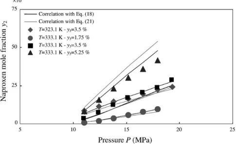
Fig. 5. Naproxen solubility vs. pressure with methanol as cosolvent: measurements and correlation withEqs. (18) and (21).
each cosolvent are treated independently withEq. (18)(lines 2–5 in Table 10). The maximum AAD is 11% for methanol, with a good representation of solubility data as illustrated onFig. 5. As observed for PC data, parameters attributed to density, B4, and to temperature, C4, seem to be nearly constant and close to that obtained for pure CO2, except for ethyl acetate for which data exist at only one temperature. Thus, a correlation withEq. (18)is carried out by gathering data for each cosolvent with the ones in pure CO2 (lines 6–9 inTable 10). This global treatment does not lead to a significant increase in the AAD, parameters A4, B4and C4being the same for both CO2used alone or mixed with a cosolvent. Then, these
three coefficients can be considered as independent of the nature of the SCF. As previously observed for the pharmaceutical compound, it confirms that the part of cosolvent effect due to specific interactions is independent of density and temperature effects, and is quantified for each cosolvent by the value of D4. Thus, the following relationship, similar toEq. (19)with seven adjustable parameters can be applied:
T ln" y2P Pstd
#
= A6+ B6ρf + C6T + D6y3ethanol+ E6y3ethyl acetate+ F6y3acetone+ G6y3methanol. (20) The AAD obtained is equal to 11.2% with 119 data and four cosolvents treated. The good fit is illustrated for acetone as cosolvent onFig. 5. This confirms the validity of this relationship, which can be written in a more general way as:
T ln" y2P Pstd # = A6+ B6ρf + C6T + % cos D6cosy3cos (21)
where superscript cos means cosolvent. By plotting T ln(y2P /Pstd)− C6T +'cosD6cosy3cos versus ρf, the 119 solubility data are gathered on a single line (Fig. 6).
4. Discussion
The application of the models to data in pure CO2 provides three relationships between C2, P and T or y2, P and T with, for given solute and solvent, constant values of three adjustable parameters. Finally, relationships obtained allow the prediction of the solubility y2 in other operating conditions.
If a cosolvent is used, the extension of the Chrastil model can be applied only to mixtures at constant composition. On the contrary, the two other models provide two relationships between y2, P, T and y3 which can be used for the calculation of the solubility under other experimental conditions, whatever the pressure, the temperature and the cosolvent mole fraction. The modified Ziger and Eckert model requires the use of a set of parameters for each cosolvent. The generalized Mendez-Santiago and Teja model allows the characterization of the solubility of a given solute in a given solvent with only one relationship for several cosolvents.
It is not possible to state a priori which model is the best among the three models described here. They are semi-empirical and it is recommended that they be tested in each individual case. In addition, it seems interesting to apply at least two of them to the same data in order to compare and to check the results obtained.
5. Conclusion
Solubility data for pharmaceutical solid have been correlated by means of three density-based semi-empirical models: the Chrastil model, the Ziger and Eckert model and the Mendez-Santiago and Teja model.
The Ziger and Eckert model has been modified to be applicable when the saturated vapor pressure of the solute is unknown. The application of the three correlations to the data in pure CO2leads to expressions which can be used for prediction purposes in a large range of pressure–temperature conditions.
In addition, the Chrastil and the Ziger and Eckert models have been extended to be applicable to solvent–cosolvent mixtures considered as pure SCF compounds. This work has confirmed the importance
of specific interactions in the cosolvent effect. Based on experimental observations, a term has been introduced in the modified Ziger and Eckert model to represent the influence of the solvent–cosolvent composition. This novel relationship has allowed a good representation of all data for each cosolvent in supercritical CO2. The representation of all the data with two different cosolvents has been carried out with only one relationship by using a generalized Mendez-Santiago and Teja model, in which effects of density, temperature and cosolvent composition are quantified.
Finally, the validity of the relationships proposed in this work has been checked with naproxen solubility data in supercritical CO2. A good representation has been found with the modified Ziger and Eckert model for all of the four cosolvents studied. The generalized Mendez-Santiago and Teja model has allowed the correlation of 119 data with four different cosolvents by using only one equation with seven adjustable parameters.
List of symbols
a energy parameter in vdW equation (J m3mol−2)
A1, B1 coefficients inEq. (4)(K, K m3kg−1) A′1, B1′, C1′ coefficients inEq. (5)(Pa K, K m2s−2, Pa)
A2, B2, C2 coefficients inEq. (7)(K, K m3kg−1, –)
A3, B3, D3 coefficients inEq. (8)(K, K m3kg−1, K)
A4, B4, C4, D4 coefficients inEq. (18)(K, K m3kg−1, –, K)
A5, B5, C5, D5, E5 coefficients inEq. (19)(K, K m3kg−1, –, K, K)
A6, B6, C6, D6, E6, F6, G6 coefficients inEq. (20)(K, K m3kg−1, –, K, K, K, K) AAD average absolute deviation, defined inEq. (9)
C concentration (kg m−3)
E solubility enhancement factor, defined inEq. (3)
EoS equation of state
i, j coefficients inEq. (6)(–, K)
k association number inEq. (1)
k1, k3 association numbers inEq. (10)
kij binary interaction parameter
lij binary interaction parameter
M molecular weight (kg mol−1)
n number of data
P pressure (Pa)
R universal gas constant (J mol−1K−1)
T temperature (K)
v mole volume (cm3mol−1)
y mole fraction
Greek letters
α, β coefficients inEq. (1)(K, –)
δ Hildebrand solubility parameter (Pa1/2)
∆ ratio of solubility parameter, defined inEq. (3) ε2 dimensionless energy parameter, defined inEq. (3) η1, ν1 coefficients inEq. (2)
η2, κ2, ν2 coefficients inEq. (13)(–, K, –) η3, κ3, ν3 coefficients inEq. (14)(–, K, –) η4, κ4, λ4, ν3 coefficients inEq. (17)(–, K, –, –) ρ density (kg m−3) ω acentric factor Subscripts
1 light solvent component (carbon dioxide) 2 heavy solute component (solid)
3 cosolvent
C critical point
cal calculated value exp experimental value f supercritical phase m solvent–cosolvent mixture Superscripts sat sublimation std standard L liquid Acknowledgements
The authors would like to acknowledge the financial and technical support of the Pierre Fabre Research Institute (IRPF).
References
[1] M. Sauceau, D. Richon, J.-J. Letourneau, J. Fages, in: K. Mallikarjunan, G. Barbosa-Canovas (Eds.), Proceedings of the AIChE Annual Meeting & 7th Conference of Food Engineering, AIChE Publication No. 151, Reno, 2001, pp. 212–217. [2] M. Sauceau, J. Fages, J.-J. Letourneau, D. Richon, Ind. Eng. Chem. Res. 39 (2000) 4609–4614.
[3] J. Chrastil, J. Phys. Chem. 86 (1982) 3016–3021.
[4] D. Ziger, C. Eckert, Ind. Eng. Chem. Process Des. Dev. 22 (1983) 582–588. [5] A. Harvey, J. Phys. Chem. 94 (1990) 8403–8406.
[6] J. Mendez-Santiago, A. Teja, Fluid Phase Equilib. 158–160 (1999) 501–510. [7] J. Mendez-Santiago, A. Teja, Ind. Eng. Chem. Res. 39 (2000) 4767–4771. [8] D.-Y. Peng, D. Robinson, Ind. Eng. Chem. Fundam. 15 (1976) 59–64.
[9] A. Kordikowski, A.P. Schenk, R.M. Van Nielen, C.J. Peters, J. Supercrit. Fluids 8 (1995) 205–216. [10] S. Ting, S. Macnaughton, D. Tomasko, N. Foster, Ind. Eng. Chem. Res. 32 (1993) 1471–1481. [11] C.J. Giddings, M.N. Myers, J.W. King, J. Chromatogr. Sci. 7 (1969) 276–283.
[12] G. Gurdial, N. Foster, Ind. Eng. Chem. Res. 30 (1991) 575–580. [13] R. Fedors, Polym. Eng. Sci. 14 (1979) 147–154.
![Fig. 3. log 10 (y 2 P /P std ) vs. log 10 (y 3 ) for naproxen solubility data with ethanol as cosolvent at 333.1 K (data from [10]).](https://thumb-eu.123doks.com/thumbv2/123doknet/11645795.307769/11.892.73.832.408.569/fig-log-naproxen-solubility-data-ethanol-cosolvent-data.webp)