On turbulence and the formation of riffle-pools in gravel-bed rivers = La turbulence et la formation des seuils-mouilles dans les rivières à lit de gravier

Université de Montréal

On Turbulence and thc formation ofRiffle-Poolsin Gravel-Bed Rivcrs (La turbulence et la formation des seuils-mouilles dans les rivières à lit de gravier)

par

Bruce J. MacVicar

Département de géographie faculté des arts et des sciences

Thèse présentée à ta Faculté des études supérieures en vue de l’obtention du grade de

Philosophiae Doctor (Ph.D.) en géographie

May, 2006

G

o

57

Université

de Montréal

Direction des bibliothèques

AVIS

L’auteur a autorisé l’Université de Montréal à reproduire et diffuser, en totalité ou en partie, _{par quelque moyen que ce soit et sur quelque support que ce} soit, et exclusivement à des fins non lucratives d’enseignement et de

recherche, des copies de ce mémoire ou de cette thèse.

L’auteur et les coauteurs le cas échéant conservent la propriété du droit

d’auteur et des droits moraux qui protègent ce document. Ni la thèse ou le

mémoire, ni des extraits substantiels de ce document, ne doivent être imprimés ou autrement reproduits sans l’autorisation de l’auteur.

Afin de se conformer à la Loi canadienne sur la protection des renseignements personnels, quelques formulaires secondaires, coordonnées

ou signatures intégrées au texte ont pu être enlevés de ce document. Bien

que cela ait pu affecter la pagination, il n’y a aucun contenu manquant.

NOTICE

The author of this thesis or dissertation has granted a nonexclusive license allowing Université de Montréal to reproduce and publish the document, in part or in whole, and in any format, solely for noncommercial educationa! and

research purposes.

The author and co-authors if applicable retain copyright ownership and moral rights in this document. Neither the whole thesis or dissertation, nor

substantial extracts from it, may be printed or otherwise reproduced without the author’s permission.

In compliance with the Canadian Privacy Act some supporting forms, contact information or signatures may have been removed from the document. While this may affect the document page count, it does flot represent any loss of

Univcsité de Montréal Faculté des études supérieures

Cette thése intitulée:

Turbulence and the Formation of Riffle-Poots in Gravet-Bed Rivets (La turbulence et la formation des seuils-mouilles dans les rivières à lit de gravier)

présentée par: Bruce]. MacVicar

a été évaluée par un jury composé des personnes suivantes:

Lael Parrott - présisent-rapporteur

André Roy- directeur de recherche

François Courchesne - membre dujury

Michel Lapointe - membre du jury

Douglas Thompson - examinateur externe

iii

RÉSUMÉ

Cette thèse doctorale porte sur l’organisation des rivières à lit dc graviers. La formation du lit en séquences à grande échelle - les séquences seuil-mouille- est une

caractéristique de ces rivières qui contrôle la stabilité et la productivité écologique. Malgré son importance, le mécanisme qui génère les seuil-mouilles reste obscur. Ce problème est lié à trois facteurs: les données dc terrain qui existentne sont pas suffisantes pour accepter ou rejeter les hypothèses qui existent; la compLexité des interactions entre l’écoulement, le transport des sédiments, et les formes dii lit; et le rôle de la turbulence qui n’est pas considéré dc façon adéquate. L’approche de cette thèse est d’aborder ces facteurs

simultanément avec des méthodes innovatrices pour mesurer les paramètres importants sur le terrain et de modéliser des processus non linéaires dans une rivière. Les objectifs sont: ta) de développer un modèle qui est capable de simuler le transport des sédiments et les interactions avec l’écoulement turbulent, (b) en utilisant le modèle, de montrer te rôle des mécanismes de rétroaction dans le développement des formes du lit, (c) de tester les vélocimètres clans des écoulements à fortes vitesses et fortes intensités turbulente, (d) de mesurer et caractériser les dynamiques de l’écoulement dans un seuil-mouille forcé, (e) de mesurer et caractériser les dynamiques de la sédirnentologie et la morphologie dans un seuil-mouille forcé, et (f’) en utilisant le modèle et l’analyse des données de terrain, d’identifier les mécanismes qui contribuent à la formation des seuils—mouilles.

En considérant une rivière comme un système complexe, nous avons créé un modèle qui simule le transport des sédiments individuellement, c’est-à-dire un modèle ‘discret’. Les particules répondent aux paramètres locaux de l’écoulement et des boucles de rétroaction sont possibles. Les processus physiques sont simplifiés afinde permettre la considération des mécanismesqui génèrent les formes dii lit. Nous montrons que les formes du lit à grande échelle émergent quand la turbulence varie en fonction de l’accélération et de la décélération de l’écoulement.

Nous avons suivi lesdynamiques d’un seuil—mouille forcé pendant I 8 mois. Cette période était très active en terme de changements géomorphologiqies à cause d’une série de crues de haut niveau. La plus grande étaitune crue d’une période de 15 ans. Nous avons échantillonné des séries de vitesses instantanées à 90 - 270 positions au site pendant des

crues de bas niveau jusqu’a plein bord. Les instruments ont été testés dans les

environnements comparables afin d’assurer leurs capacités de fonctionner comme prévu. Les données hydrauliques nous ont montré quelques résultats importants. La décélération et l’accélération définissent respectivement l’écoulement dans le début et lafin de la mouille. Ceci a un effet importantsurla forme des profils de vitesse moyenne, où des vitesses relativement basses sont présentes prochedu lit dans la zone dc décélération et des vitesses relativement hautes sont présentes proche du lit dans la zone d’accélération. Cet effet explique les observations d’un renversement de vitesses. Cependant, le renversement de vitesses est présent seulement dans la zone vers la finde la mouille où la pente du lit est positive. Pour expliquer le transport des sédiments dans le début de ta mouille, un effet secondaire est requis. Dans cet environnement, l’intensité de la turbulence est haute. Nous avons observé la séparation intermittente de l’écoulement dans cette région de l’écoulement et il apparaît que cette zone génère la turbulence observée.

Afin de suivre les mouvements des particules et de caractériser les patrons spatiaux du transport des sédiments, nous avons utilisé une technique relativement nouvelle basé sur les ‘Passive Integrated Transponder (PIT) tags’. Nous avons marqué 300 roches de

différentes tailles. Nous avons aussi cartographié le lit de la rivière plusieurs fois pendant cette même période afin de suivre tes changements morphologiques. Un événement majeur s’est passé au début de la période d’étude. Cet événement a déplacé l’arbre qui détermine Le lieu de la mouille, ce qui a provoqué une nouvelle période de développement

morphologique qtie nous avons caractérisée. En général, la morphologie et le transport de sédiment reflètent la variabilité de l’écoulement. En aval de l’arbre, toutes les tailles de particules marquées ont été enlevées de la mouille et l’érosion de la mouille à été progressive. En contraste, en amont de l’arbre nous avons observé que le transport de sédiment est très sensible aux tailles des particules et que deux cycles d’aggradation et de dégradation se sont produits. Les particules plus larges que le D n’ont pas été déplacées du début de la mouille pendant la période d’études, malgré au moins un événement avec une fréquence de retour de 15 ans.

La conclusion centrale de la modélisation et de l’étude de terrain est que la

turbulence est nécessaire pour expliquer la formation des seuil-mouilles. Le modèle est très important pour la généralisation des résultats parce qu’il démontre que des formes du tit

V

avec une taille, un triage de particule par taille, et une stabilité similaire à ce que nous observons dans les seuil-mouilles naturels peuvent être générées sans qu’un élément comme l’arbre soit présent pour le provoquer. Pour cela, il faut que le modèle inclue une règle qui lie la turbulence à l’accélération, une autre règle qui imite l’effet de la séparation de l’écoulement, et les sédiments de tailles hétérogènes. La convergence de ces facteurs avec les observations de terrain encourage l’hypothèse que tous les seuil-mouilles sont générés par un mécanisme similaire. Il apparaît que les éléments qui forcent les seuil-mouilles fonctionnent comme des catalyseurs qui activent les processus associés à l’écoulement non uniforme, mais que ces processus peuvent aussi émerger du système complexe qui

constitue une rivière à lit graveleux. Ces résultats sont uniques dans la littérature et portent une nouvelle vision sur les dynamiques fluviales, la complexité, et l’organisation d’une rivière.

Mot-clés: rivières à lit graveleux; seuil-mouille; turbulence; système complexe; transport de sédiment; pistage de sédiment; formes du lit; cohérence; mesure de vitesse; écoulement non uniforme; accélération; décélération; séparation intermittente; émergence; auto-organisation.

SuMMARY

This thesis is a study of organization in rivers. Riffic-pool sequences determine the macro-scale structure in a broad range ofgravel-bed rivers. Thcy arc dcflncd by a scaling relation with stream width, sorting of sediment by size, and the formation of lateral bars. These features are of intercst because thcy excrt a significant control on stream stability and ecology. In spite of considerable effort, there is no consensus on the rncchanism(s) by which the forms develop and are maintaincd. This problem is retated to three factors: field data that is inadequate to accept or reject proposed hypotheses, the complexity ofthe possible interactions between the flow, sediment transport and bed form development, and inadequate consideration ofthe cffects of turbulence. The approach of this thesis is to address these factors simultaneously through new modetiing strategies and improved fictd methods and measurements. The specific objectives are: (a) to develop a rnodcl to simulate flow and sediment dynamics in order to examine the dynamics ofbcd form devclopment in gravel-bed rivers and to demonstrate the role of feedback mechanisms in bcd form

development including the effect of turbulence; (b) to test available instrumentation for measuring turbulent flow properties in gravcl-bed rivers during floods; (c) to measure and characterize the mean and turbulent flow dynamics ofa forced rime-pool and the sediment and morphologic dynarnics in a forccd riffic-pool; and (d) to use both the numerical simulations and analysis ofthe ficld data, to idcntify the mechanisms that lead to the formation and maintenance ofriffle-pools in gravcl-bcd rivers.

Based on the assumption that a gravel-bed river may be described as a complex system, we developed a discrete particle mode! that simulates the transport ofindividual particles based on local mies to determine particle entrainrnent and the fecdbacks between flow and bed form development. Physical processes were simplified to allow us to consider the mechanisms by which bed forms occur and are maintaincd. The model is capable of generating a wide range ofbed forms at different scales. By varying turbulence intensity in response to iow acceleration and deceleration, we demonstrated the emergence ofmacro-scaie bed forms.

To measure and characterize the flow and sediment dynamics ofriffle-pools, we monitored a forccd riffle-pool intensely for an 1 8 moith period. The site is located in

vii Moras Creek, a 6 ni wide gravel bed stream near Victoriaville (Quebec). The location of the riffle-pool is forced by a large tree with an intact root wad that sud in to the stream. The study pcriod was geornorphica[Ïy active. At the beginning of the study period, a large flood event rotateded the tree and reinitiated pool scour. A series of subsequent events, the largest ofwhich had a return period of approximately 15 years, changed pool gcometry. We sampled series of instantaneous velocity at up to 270 points through the study site during floods as high as the bankfull level. To measure velocity, we used Electromagnetic Current Meters (ECMs). These instruments were tested incomparable highly turbulent environments to ensure accuracy. The hydraulic data from the forced riffi e-pool yielded a number ofimportant and original results. Flow deceleration and acccteration were found to

dominate the pool-head and pool-tail, respectively. This has a strong effect on the shape of mean velocity profiles, such that reiatively low velocities occur near the bed in deceterating flows while retatively high velocities occur near the bed in acceicrating flows. This effect explains the occurrence ofa near-bcd velocity reversai between the riffle and the pool-tau. However, mean velocity is not adequate to explain sedirnent transport in the pool-hcad. Instead, we observed high turbulence intensities, and it appears that intermittent flow separation near the bed generates high amplitude and short duration turbulent fluctuations that may be sufficient to initiate sedirnent transport.

To tag and track the movernents of sediment particles, we utilized a reiativetynew technique based on Passive Integrated Transponder (PIT) tags. We followed morpÏiological changes during the study period by repeatedly surveying the bcd topography. Morphology and sediment transport rdflect the observed variability of flow hydraulics. Downstrearn of the tree, ail sizes of taggcd particles were evacuated from the pool center and tau on at least two occasions and progressive crosion takes place so that the pool increased in Iength through the study period. In contrast, the region upstrearn of the trcc was characterizcd by altemate cycles of scour and fill and highly size-seiective sediment entrainment. Tagged particles larger than the D84 wcrc not transported out ofthe pool-head during the study period in spite oC events as large as the 15 year flood.

The key conclusion from both the numerical modelling and the field study is that turbulence is a critical factorinthe formation ofriffle-pools. Sediment transport by high turbulence in zones of low mean vclocity appears to initiate pool scour and selectively

transport the finer sediments out of the pool-head. Thc numerical modet is criticat in the generalization of resuits because it demonstrates that bed forrns with similar size, sorting, and stability to riffle-pools can emerge in the absence of forcing elements if thrcc elcments are included: 1) a rule that links acceleration to turbulence intensity,2) flow separation

downstream ofstcep 1cc slopes, and 3) heerogeneous sediments. The convergence of modeling resuits with ficld observations encourages the conclusion that acceteration and dcccleration combincd with turbulence gcneration arc at the core ofa gencral modcl of riffle-pool formation. Forcing elcmcnts appear to act as a catalyst to activatc processes associated with nou-uniforrn flow that eau also emcrgc from the complex system ofa gravel—bed river. These results arc unique in the literature and offer a new insight into thc flow and sediment dynamics, complcxity, and organization ofa gravel-bcd river system.

key words: gravel-bcd river; riffle-pool; turbulence; complex systems; sediment transport; bed forms; cohercncc; velocity measurement; scdiment tracking; non-unifom flow; accclcration; deceleration; intermittent separation; cmcrgence; seif-organization.

ix

TABLE 0F CoNTENTs

RÉSUMÉ 111

SUMMARY VI

TABLE 0F CONTENTS IX

LIST 0F TABLES XIII

LIST 0F FIGURES XIV

NOMENCLATURE XXIV

ACKNOWLEDGEMENTS XXVIII

1 INTRODUCTION I

2 BACKGROUND 5

2.1 C0NTExI: THE GRAVEL-BEDRIVER 5

2.1.1 Turbulent flou’ oi’erugra’e1 hed 5

2.1.2 Sedinient transportingravel—bedriiers 13

2.1.3 Bedfàrindei’elopment 1)

2.2 RIFFLE-nooc MORPHOLOGY 1$

2.3 SEDIteIENT TRANSPORT IN RIFFLE-POOLS 25

2.4 FLow DYNAMICS 0F RIFFLE-POOLS 28

2.5 FORMATION 0F RIFFLE-POOLS: ‘FHEORY AND FIELD EVIDENCE 37

2.6 M0DELLING 42

2.7 PIi.0I3LEM IDENTIFICATION 48

2.8 OBJEcTIvEs 4$

2.9 METH0D0L0GY 49

2.10 TFIEsI5STATEMENT 52

3 A 2-D DISCRETE PARTICLE MODEL 0F GRAVEL-BED RIVERSYSTEMS 55

3.1 INTRODUCTION 55

3.2 GRAvEL BED FORMS 57

3.3 MoEL DESCRIPTION 5$ 3.3.1 Conceplual Approuch sS 3.3.2 InitialConditions 60 3.3.2.1 Simcilation Matrix 60 3.3.2.2 flowStagc 61 3.3.3 IvkdelAlgorithms 62

3.3.3.2 Particle 1-liding .63

3.3.3.3 Particlc Imbrication 64

3.3.3.4 Local tnstantaneous Velocity 65

3.3.3.5 Turbulence 65

33.3.6 Flow Acceleration 66

3.3.4 Stuninan ofAfodel Execution 67

3.4 Mo St1uLATloNs 68 3.5 Rsuiis 69 3.5.1 Sparc-TOue Plots 69 3.5.2 Profile plots 76 3.5.3 Roughness 78 3.5.4 Pool dimensions 79 3.5.5 Sensitivity 82 3.6 EMERGENTBEDF0RMS 83 3.7 Discussio’t 85 3.6 CoNcLusioNs 90

4 MEASURING WATER VELOCITY IN HIGHLY TURBULENT FLOWS: FIELD

TESTS 0F AN ELECTROMAGNETIC CURRENT METER (ECM) AND AN ACOUSTIC

DOPPLER VELOCIMETER (ADV) 92

4.1 INTRoDucTIoN 92

4.2 METH0D0L0GY 94

4.2.1 Field Site and Experioic’ntcil Design 94

4.2.2 SignalProcessing 97

4.2.3 DataQualiir Analrsis 98

4.2.4 Coinparison ofTurbulence Statistics 103

4.3 Rusucis 104

4.3.1 Internal ADV Paraoiete,s 104

4.3.2 Spectral Anali’sis 105

4.3.3 Error Analvsis 109

4.4 Covwiousor’t 0F TuRBuLEN1 Fww PARAMETERsANDDiscussioN 111

4.5 CoN4ccusio 117

5 FLOW DYNAMICS0FA FORCED POOLINA GRAVEL-BED RIVER PARTA:

MEAN VELOCLTV AND TURBULENCE INTENSITY 120

5.1 INTRODUCTiON 120

5.2 Mi-FHODOLOGY 122

5.2.1 field Site 122

xi

5.2.3 DataQualitv anti Post-Processing 129

5.2.4 Ttirbulenceintensitvaiîdshear .çtresshinon—toufrmflou’ 130

5.3 RESULTsANDANALYsIs 133

5.3.1 Spatïal a,idflow Stage Variabilitj’ 133

5.3.2 Mean velocityproJfles at bankjidlfirn 139

5.3.3 Efii.’ct offioodstageon innerflowregioli 140

5.3.4 Turbulence intensit)’ andshear stress 142

5.4 DiscussioN 145

5.4.1 Streaniwise velocity profiles 146

5.4.2 Laterally com’ergingflow andsecondaiy circulation 148

5.4.3 Turbulence genera1io1 and energl’dissipation 149

5.4.4 ShearStressinNon—UnijormFloi 150

5.5 CottcLusioNs 152

6 FLOW DYNAMICS 0F A FORCED POOL IN A GRAVEL-BED RIVER PART B:

THE STRUCTURE AND SCALE 0F TURBULENT EVENTS 154

6.1 INTRODUCTION 154

6.2 METH0DOL0GY 157

6.2.1 Field Site and Data Collection 157

6.2.2 Modelofineanvelocitv anti ttnbulence intensit, 158

6.2.3 Data Anah’sis 159

6.2.3.1 flowSeparation 159

6.2.3.2 Spectral analysis 160

6.2.3.3 Space-time correlation and auto-correlation 160

6.2.3.4 Eent Analysis 161

6.3 REsucis 163

6.3.1 Flou Separation 163

6.3.2 Spectralanalysis 165

6.3.3 Space—tinie correlationandanta—correlation 168

6.3.4 Ei’ent anal)’sis 173

6.3.5 Efjict ofdischarge 184

6.4 DiscussioN 186

6.5 CONCLUSION 189

7 SEDIN1ENT DYNAMICS 0f A FORCED POOL IN A GRAVEL-BED RIVER 192

7.1 INTR0DtJcTI0N 192

7.2 METH0D0L0GY 194

7.3 Rsuiis 204

7.3.2 Patli lengths nI sedi,,ient transport. 208

7.3.3 5atia1 distributionof c’ntrainmentand deposition oftaggedpartic/es .110

7.4 DiscussioN 216

7.5 CoNciwsios 222

S GENERAL DISCUSSION AND CONCLUSIONS

8.1 INTRODUCTION 223

8.2 SUMMARY 0FKEY FINDINGS 223

8.3 ORIGINALITY 0F THE THEsIs 226

8.4 CoNcErTu.\c MODEL 228

8.5 FuTURE RESEARCH 229

BIBLIOGRAPHY 233

APPENDIX A-ACCORD DES COAUTEURS ET PERMISSION DE L’ÉDITEUR 250

APPENDIX B-AUTORISATION DE RÉDIGER LA THÈSE EN ANGLAIS 255

APPENDIX C- AUTORISATION DE RÉDIGER LA THÈSE SOUS FORME D’ARTICLES

xiii

LIST 0F TABLES

TABLE2.1 - ENIPIRICALSTUDIES 0F POOL-RIFFLE MORPHOLOGY 19

TABLE2.2-MORPHOLOGY AND EXPERIMENTAL DESIGN 0F FIELD-BASED STUDIES 30

TABLE2.3 - M0DELLING STUDIES RELEVANT TO RIFFLE-POOL MECHANICS 45

TABLE3.1- DISCRETE PARTICLE MODELS IN FLUVIAL ENVIRONMENTS 54

TABLE3.2 -GRAvEL BED FORMS 56

TABLE3.3—ROQ-B INAL PARAMETERs 59

TABLE3.4—ROQ-3C0NTIWL PARAMETERS 62

TABLE4.1 -PAsT STUDIES COMPARING THE PERFORMANCE 0FADVsANDECMs 92

TABLE4.2-PARAMETERs FOR ESTIMATION 0FADVMEASUREMENT ERRORS 99

TABLE4.3-VARIANCE BETWEEEN ECMANDADVDATA 112

TABLE4.4 - SusîrIARY 0F CONTRIBUTIONS B’’ QUADRANT 114

TABLE5.1- SuMrl,Ry 0F FLow SArlrLING DATES 125

TABLE5.2-PARAMETER5 0F FLOW PROFILES 126

TABLE7.1 -SuMMARY 0F FLOOD SEQUENCES BETWEEN SURVEYS 196

TABLE7.2 -SAMPLE5 0F TAGGED PARTICLES BY SIZE CLASS 197

LIST 0F FIGuREs

FIGURE2.1 -C0NCEPTUAL MODEL 0F INTERACTIONS BETWEEN FLOW, RFPRESENTED BY A MEASURED TIME

SERIES 0F INSTANTANEOUS VFL0CITIES PARTICLE M0\’EMENT, REPRESENTED BY INDI\’IDUAL PARTICLLS, AND BED FORM DE\’ELOPMENT, REPRESENTED BY A RIFFLE-POOL UNIT (FROM LECDER, 1983) 5 FIGURE2.2-C0NCEPTUAL DIAGRAM 0F REGIONS IN TUE FLOW FIELD AND COORDINATE SYSTEM 7

FIGURE2.3-VEL0CITY PROFILES FOR UNIFORM AND NON-UNIFORM FLOWS[KI1?oNoTo.1vD GR.-IF, 1995] 7

FIGURE2.4-NORMALIzED REYNOLDS SHEAR STRESS IN UNIFORM FLOW VERSUS DEI’TH [NEzUAND N1KAG1JV1,

19931 8

FIGURE2.5-DISTRIBUTION 0F TURBULENCE INTENSITIES IN UNIFORM FLOW 0VER SMOOTH AND ROUGH BEDS

[NEzu1NDN,1K,4G,4IvA, 1993] 9

FIGURE2.6-TURBULENcE INTENSITIES AND NORMALIZED REYN0LD5 SHEAR STRESS DISTRIBUTIONS IN NON

UNIFORMFLOW[KIRONOTO1WDGRÀE, 1995] 10

FIGURE2.7-SUCCESSIVE LAYERS 0F TUE FLOW NEAR A FLAT PLATE[KLINE ET,IL., 1967] 11

FIGURE2.8-TURBULENT BOUNDARY LAYER ON A WALL[FALC0, 1977] 12

FIGURE2.9-AFLOW MODEL IN SEPARATING FLOWS[S1I1PsoN ETAL., 1981]. IDDENOTES INCIPIENT

DETACHMENT, lTDDENOTES INTERMITTENT TRANSITORY DETACHMENT ANDDOENOTES DETACHMENT.

12

FIGURE2.10-DOwNSTREANI VARIATION 0F THE VIRTUAL VELOCITY FOR TAGGED SEDIMENT BY SIZE CLASS

EFERGUSONANDH0EY,20021 13

FIGURE2.11 - BEDL0ÀD TRANSPORT AS A FUNCTION 0F SIREAM POWER FOR DArA SETS USED INGoMIEz-IVD

Cîuitcn[1989] 15

FIGURE2.12-AUNIFIED BLD FORM PHASE DIAGRAM ACROSS A RANGE 0F SAND AND GK,\VEL SIZES [BE5T,

1996] 16

FIGUIE2.13 -MEASUIŒD DISTRIBUTIONS 0F STREAMWISE VELOCITY, REYNOLUS SHEAR STRESS, AND NORMAL

STRESS (U’2) OVER FIXED DUNE FORMS [NcLsoNETlL., 1993] 17

FIGURE2.14-SCHENIATIC DIAGRAM 0F TUE PRINCIPAL REGIONS 0F FLOW OVER ASYMMETRICAL DUNES[BEsT,

2005] 18

FIGURE2.15-Fcow REGIONS ASSOCIATED WITH 1HE PRESENCE 0F A PEBBLE CLUSTER[BUFFIN-BÉL1NGER AND

Ro, 1998] 18

FIGURE2.16—VIsUALIzATI0N 0F TRACERS IN LOWER LEE AND TROUGH 0F LOW-ANGLED DUNE SHO\VING INTERMITTENT FLOW SEPARATION [BESIINDKosTIscneK,2002] 18

FIGURE2.17-SCHEtATIc DIAGRAM T0 DEFINE THE RIFFLE-POOL SEQUENCE[CHLRCu1vDJo,vEs, 1982] 21

FIGURE2.18 -ADESCRII’TI\’E MODEL 0F SEDIMENT TRANSPORT PROCESSES IN A RIFFLE-POOL[SEAR. 1996]....21

FIGURE2.19-STÀ\C;Es IN FORMATION 0F A BAR SHOWING HE DEPOSITION 0F A COARSE BAR HEAD ATH[ListE

ET-IL., 1991] 23

xv FIGuRE2.21 -AFIVE-STAGE MODEL 0F DEVELOPMENT THAT SHOWS A PROGRESSION FROM ALTERNATE BARS

10 MEANDERING [KELLER,1972] 25

FIGURE2.22-CHANGES IN STORAGE 0F BED SEDIMENT IN RESPONSE 10 CHANGES IN WAFER DISCHARGE ON

THREE MAJOR RIFFLES (LEFT) AND THREE MAJOR STORAGE AREAS (RIGHT) IN THE EAST F0RK RIVER

[AlCADE, 19851 27

FIGURE2.23-COIPARIsON 0F DISCHARGE VERSUS SEDIMENT TRANSPORT RELATIONS FROM(A)RE.INET.IL.

[2002]AND(B)].1CKSO;V.1,VDBESCHTJ [1982] 27

FIGuRE2.24-BLD SHEAR STRESS NEEDED 10 INITIATE AND TO FULLY MOBILIZE SEDIMENTS IN A POOL VERSUS

GRAIN SIZE[H.Isstw..IND WOODSAIITH,2004]. ALS0 SHOWN ARE RESULTS FROM FLUME EXPERIMENTS

[WILCOcKANDMCARDELL, 19931,AND KARRIS CREEK[C[IuRCII,.liVo Hlss1N,2002] 28

FIGURE2.25-WIDTH \‘ERSUS SLOPE FOR HYDRAULIC STUDIES 0F RIFFLE-POOLS AS LISTED IN TABLE2.2.

PARTICLE SIZE(D50)AND POOL TYPE ARE SHOWN FOR EACH SITE. RELATIONS A AND B FOLLOWING WERE FIT BY EYE 10 THE DATA. M0RAS CREEK, THE STUDY SITE IN THIS THESIS, IS ALSO

32

FIGURE2.26-VEL0CITY PROFILES AT POOL AND RIFFLE CROSS-SECTIONStBH0,1ICK.1ND DEAIISSIE, 19621 33

FIGURE2.27-SPATIALLY AVERAGED VELOCITY PROFILE FOR POOLS AND RIFFLES DURING HIGH FLOW

CONDITIONS(O2/3 O,s,)[1?01T, 1997] 34

FIGURE2.28-N[AR-BEO VELOCITIES MEASURED AT(A) LOW FLOW (B) NIODERATE FLOW (C) HIGH FLOW

A STRAIGHT RIFFLE-POOL AlRM -RIFFLE MIOPOINT,RC-RIFFLE CREST,PT-POOL-rAIL,

PM-POOL MIDPOINT[CLifEoRD.IvD RICHiIt)s, 1992]. FLOwIS FROM RIGHT TO LEFT AND THE HEIGHT

0F THE BAR REPRESENTS THE VELOCITY 34

FIGURE2.29-VARIATION IN ABSOLUTE TURBULENCE INTENSITY(RMS IN MIS) THROUGH FWO RIFFLE-POOLS

DURING MODERATE DISCHARGE[CUFF0RD, 1996]. FLOW DIRECTION IS FROM RIGHTTO LEFT. CL0SED SYMBOLS REFER TO STREAMWISE VELOCITY COMPONENTS AND OPEN SYMBOLS REFER TO \‘ERTICÀL

COMPONENTS 36

FIGuRE2.30-PLAN-VIEw MAPS 0F 10CM, 40CM,AND 70CM LONG POOLS SHOWING VELOCITY VECTORS FOR

THE STREAMWISE AND LATERAL COMPONENTS 0F NEAR-BED (BLACK ARROWS) AND 0.4Y(wHITE ARROtVS) VELOCITIES. THE ARROWS ARE SUPERIMPOSED ON TURBULENT KINETIC ENERGY(EjAl0.4)’

[TIiowPsoN,2004] 36

FIGURE2.31-THE EFFECT 0F AN INCREASE 0F lIME ON PAFH LENGTH DISTRIBUTIONS [EIvsTEIN, 19371. TIME

INCREASES FROM A-F. [PI’RCE-IvDAsnÂIoRE,20031 38

FIGURE2.32-CHANNEL WIDTH \‘ERSUS MO[)ES 0F TRANSPORT DISTANCE FROM STUDIES COMPILED BYPI’xcE

ASHIfORE[2003] 39

FIGURE2.33-VEL0CFFY REVERSAL HYPOTI-IESIS FOR A RIEFLE-POOL IN DI CREEK[Ki1JER, 1982]. THE

DATA INKELLEI?[1971]DO NOT EXTEND PAST THE THRESHOLD POINT AND THE DASHED LINES HAVE NOT

FIGuRE2.34-NEAR-BED VELOCITY AI CHANNEL CENTERLINE IN RIVER QUARME AIRM-RIFFLE MIDPOINT,

RC-RIFFLE CRESI,PT-POOL-TAIL, ANDPM-POOL MIDPOINI[CUFF0RD.4NDRJCI-1.1RDs, 1992]. ONLY

THE POOL-TAIL ALWAYS INCREASES WITH DISCHARGE 41

FIGURE2.35-M0DELLED CROSS-SECTIONAL AREA, VELOCITY, AVERAGE NEAR-BED VELOCITY, AND SHEAR

STRESSAI MID-RIFFLE(R)AND MID-POOL(P)CROSS-SECTIONSEBOOKER ET,1L.,2001] 43

FIGuRE2.36-APERPECTIVE VIEW 0F BED TOPOGRAPHY 0F ALTERNATE BARS PREDICTED BY 111E SIABILITY

MODELOFCOLUMBINJET.4L.[1987] 44

FIGURE2.37 -AN EXAMPLE 0F THE BED IOPOGRAPHY GENERATED BY IRE DISCRETE MODEL 0F A1DEN(1987J.

45

FIGURE2.38 -IMAGE 0F MIXED SEDIMENI-SIZE BLD DURING MODELLED TRANSPORT[ScHMEEcKLE..lvD

NELSON,2003] 46

FIGURE2.39-DUNE DEVELOPMENT IN A DICRETE PARTICLE MODEL IN WHICH SIMPLE RULES ARE USED 10

REPRESENI AEOLIAN TRANSPORT[ANDERS0N AND BUNAS, 1993] 46

FIGURE3.1 -RELATION 0F VELOCITY PROBABILITY DISTRIBUTIONS 10 MOVEMENT MODE IHRESHOLDS AT

IHREE FLOW STAGES FOR IHREE PARIICLE SIZES. THI5 FIGURE REPRESENTS EQUATIONSI AND2 WHEN FEEDBACK RULES ARE INACTIVE. SALTATI0N PATHS ARE SHOWN IN FIGURE3.5 MEDIUM AND LARGE PARIICLES HAVE A ‘HANDLE’ ON IHE UPPER RIGHI CORNER, AND IRIS HANDLE IS DARKENED SLIGHILY

TO AID IRE DISTINCTION 0F INDIVIDUAL PARTICLES 60

FIGURE3.2-SCHLN1AI[C DIAGRAM 0F MODELED FLOW AND PARTIC’LE FEEDBACK MECHANISMS 60

FIGURE3.3-INITIAL SIMULATION MAIRIX SHOWING DEFAULI MAIRIX DIMENSIONS, PARIICLE SIZE

DISTRIBUTION (PERCENIAGES 0F EACH SIZE CLASS INDICAIED DVI),AND BED SLOPE(5’). FLOW S FROM

LEFI 10 RIGHI 61

FIGURE3.4-DEFAULI RYDROGRAPH SHOWING SIX PYRAMID-SHAPE FLOODS 62

FIGURE3.5 SALTATI0N PAIHS FOR - . THE PATHS ARE THOSE FOLLOWED, FROM LEFI TO RIGRT, BY THE PARIICLE HANDLE (IRE UPPER RIGRICORNER 0F MEDIUM AND LARGE PARTICLES). TRE OCCUPATION 0F A GRID SQUARE IN IRE PAIR 0F ANY PART 0F THE PARIICLE WILL TERMINATE SALTATION AND INDUCE

DEPOSITION 63

FIGURE3.6- FI\’E EXAMPLES, TWO FOR SMALL PARTICLES (lxl)AND IHREE FOR LARGE PARIICLES (3x3),

SHOWING IRE CALCULATION 0F BURIAL DEPTH (y11) FOR DETERMINATION 0F HIDING FACIOR. PARTICLES

ARE SHADEI) AS FOR FIGURE3.1 64

FIGURE3.7-CALCULATI0N 0F IMBRICATION. FOR PARIICLE INDICATED BY

,_{PARTICLES IN CRAIN UPSIREAM}

(M)= I ANI) PARi ICLES DOWNSIREAM IN CRAIN(N) 3. USING EQUATION3.4ANDK1=0.5: J=3(0.5+

0.5 +0.52-b 0.53) =4.125 65

FIGURE3.8-ExAMPLE 10 DEMONSIRAIE FLOW FEEDBACK RULE CALCULAIIONS. (A) DASHED LINE- WAIER

SURFACE; SOLII) LINE-BLD SURFACE; (B) TURBULENCE RULE WITH CONIROL PARAMETER (x1)=3.0

(BLACK LINE-MEAN VELOCITY V;WHITE LINE- DEPTR AVERAGED VELOCITY VD;GREY BARS

-STANDARD DEVIATION);(C) ACCELERATION RULE WIIH CONIROL PARAMETER(K4)=0.003,ANDK 3.0;AND(D) INSTANTANEOUS VELOCITY SAMPLES; (+IuRBULENCE RULE; ACCELERATION RuLE) 67

xvii

FIGuRE3.9- FLow CHART 0F MODEL EXECUTION .68

FIGuRE3.10-SPAcE-TIME PLOTS 0F BLD SURFACE ELE VATIONS FOR BASIC MODEL SIMULATIONS. BLD

SURFACE ELEVATIONS HAVE BEEN NORMALIZED DV REMOVING THE MEAN SLOPE AND DIVIDING BY THE LARGEST STANDARD DEVIATION OFTHE FINAL BED SURFACES IN THE SERIES(YISs*). ACCUMULATIONS 0F PARTICLES ABOVE THE MEAN SLOPE APPEAR WHITE, WHILE POOLS ARE DARK. FINAL SURFACE PROFILES ARE INCLUDED FOR EACH SIMULATION RUN TO AID INTERPRETATION 0F THE GRAPHICS. FLOw

DIRECTION IS FROM LEFT 10 RIGHT 71

FIGURE3.1 1 -SPACE-TIME PLOTS 0F y/*FOR HIDING RULE SIMULATIONS. SEE CAPTION 0F FIGURE3.10FOR

MORE DETAILED EXPLANATION 72

FIGURE3.12 -SPACE-TIME PLOTS 0F y9/sFOR IMBRICATION RULE SIMULATIONS. SEE CAPTION 0F FIGURE3.10

FOR MORE DETAILED EXPLANATION 73

FIGURE3.13-SPACE-TIME PLOTS 0F )/S* FOR TURBULENCE RULE SIMULATIONS. SEE CAPTION 0F FIGURE3.10

FOR MORE DETAILED EXPLANATION 74

FIGURE3.14-SPACE-TIME PLOTS 0F IJSt FOR ACCELERATION RULE SIMULATIONS. SELCAPTION 0F FIGURE

3.10FOR MORE DETAILED EXPLANATION 75

FIGUIŒ3.15-PROFILE PLOTS ATTWO DIFFFRENT SCALES. SMALL, MEDIUM, AND LARGE PARTICLES ARE

COLORED GREY, YELLOW, AND RED, RESPECTIVELY. (A) BASIC MODEL (K1= 1, 1=2000,x=7000- 7800); (B) HIDING RULE (Kjj=3, 1=3000,x=5000-5800);(C) IMBRICATION RULE (K, 0.60, r2500, x 4500 -5300);(D) TURBULENCE RULE (K1=3 ;1=3000 ; x= 1500- 2300); (E) TURBULENCE RULE(KT 5,T

2750, x= 4850- 5650);AND (F) ACCELERATION RULE (K4=0.0004,_KT 5, i3000, x 7000- 7800)...77

FIGURE3.16-SPATIAL ROUGHNESS AS CALCULATED USING EQUATI0N3.1 1 AND A \VINDOW SIZE 0F20GRID

SQUARES. SELEcTED CASES ARE AS IN TABLE3.4 79

FIGURE3.17-Box PLOTS 0F SPATIALLY DISYRIBUTED ROUGHNESS VALUES. THE HORIZONTAL LINES THROUGH

THE BOXES REPRESENT THE MEDIANS AND THE LIMITS 0F THE BOX ARE SET AT THE INTER-QUARTILE RANGES. THE WHISKERS ARE TWICE THE QUARTILE RANGES AND + MARKERS INDICATE VALUES BEYOND

THESE LIMITS 79

FIGURE3.18-POOL DIMENSIONS(Li-”AND Yp’)VERSUS TIME FOR THE FIVE SIMULATIONS AS SELECTED IN

TABLE3.4 81

FIGURE3.19- POOL DIMENSIONS PLOT SHOWING WEIGHTED MEAN LENGTHS(Li”)AND DEPTHS(YP’)OF

RESIDUAL POOLS ON THE FINAL BLD SURFACE(1=3000)0F BASIC MODEL AND FEEDBACK SIMULATIONS. THE CONTROL PARAMETER VALUE INCREASES FROM A-D (vALUES ARE LISTED IN TABLE3.4). NoTE

THAT THE Y-AXIS IS REVERSED SO THAT LONGER AND DEEPER I’OOLS PLOT TOWARDS THF BOTTOM RIGHT HAND CORNER. ERR0R BARS ARE SHOWN IN BLACK FOR CASES SELECTED FOR RFPEAT SIMULATIONS. ERR0R BARS WERE SET AT 1.64TIMFS THE STANDARD DEVIATION 0F TI-IE WEIGHTED MEAN POOL

DIMENSION 10 ENCOMPASS95%0F THE \‘ARIABILITY 82

FIGURE3.20-SENSITIvITY TO INITIAL PARAMETERS: (A)K,= 1,(D) K11= 3,(C) K1=0.60,(D)K7=3,AND (E)K4

=0.0004. AXES REPRESENT THE I)IFFERENCE BEFWEEN MEAN POOL DIMENSIONS(Li”ANI) Y,”)

CALCULATED FROM THE REPEATABILITY SIMULATIONS. THE DIFFERENCES ARE NORMALIZED BY THE STANDARD DEVIATIONS 0F THE DIMENSIONS AS CALCULATED FROM THE REPEATABILITY SIMULATIONS

(SL’). SIrIULATIoNs WERE CONSIDERED SENSITI VE TO THE INDICATED PARANIEFER \VHERE THE

DIFFERENCE WAS GREATER THAN THE ERROR BARS (A=0.05). INITIAL PARANIETER \‘ALUES USED IN

THESE SIMULATIONS ARE LISTED IN TABLE3.4 83

FIGURE3.21 -HIGH SALTATION 0F LARGE PARTICLES VERSUS THE IMBRICATION RULE CONTROL PARAMETER (K,). K 2 FOR ALL SIMULATIONS IN THIS FIGURE. HIGFI SALTATIONS 0F LARGE PARTICLES ARE DEFINED AS THOSE WHICH ARE SUFFICIENT FOR A LARGE ‘ARTICLE TO SALTATE OVER ANOTHER LARGE PARTICLE

84

FIGURE3.22-SPACE-TIME AND PROFILE PLOTS 0F TWO SIMULATIONS TO DEMONSTRATE THE VELOCITY

PROFILE/FLOW SEPARATION RULE. THE TRIMODAL SEDIMENT IS THAT USED IN THE OTHER SIMULATIONS. THE BIMODAL SEDIMENT CONSISTS 0F40%SMALL AND6OEY0MEDIUM SIZED PARTICLES. ALL OTHER PARAMETERS ARE HELD CONSTANT IN THE TWO SIMULATIONS. PARTICLES ARE COLORED BY SIZE ON THE PROFILE PLOTS (SMALL-LIGHT GRAY; MEDIUM-DARK GRAY; AND LARGE-BLACK) 89

FIGURE4.1 -E.TON-NoRD RIvER FIELD SITE LOOKING UPSTREAM 95

FIGURE4.2-NIcOLET RIVER FIELI) SITE LOOKING DOWNSTREAM AND SAMPLING SECTION BATHYMETRY. NOTE

JET 0F WATER AS A RESULT 0F CONSTRICTION 0F FLOW BETWEEN TWO LARGE BOULDERS. SAMPLING

LOCATIONS ARE SHOWN 96

FIGURE4.3-WADING ROD WITHADVAND THREEECMs. ONLY THE ECM(AI25 CM) WAS USED FOR

THIS STUDY 96

FIGURE4.4-EFFECT 0F QUALITY ASSURANCE PROCEDURE ON TYPICAL SIGNAL. DASHED LINES FACILITATE

COMPARISON WITH K0LIoIGoR0vs-5/3 LAW ANDF,THE FREQUENCY AT WHICH THE LARGER

SAMPLING VOLUME 0F THEECMSHOULD REDUCES,.DV 10%.A)ECMSIGNAL OUTPUT; (B)ECMSIGNAL AFTER REMOVAL 0F INFERNAL FILTERING (NOTE SMALL INCREASE 0FS,NEARf)AND THE RAWADV

SIGNAL; (C’)ECMANDADVSIGNALS AFTER DE-SPIKING PROCEDURE; (D)ECMANDADVSIGNALS AFTER FILTERING WITH THIRD ORDER BUT’FEICwoRTH FILTER 99

FIGURE4.5-ESTIMATION 0F TOTAL VARIANCE DUE TO NOISE (T/) USING THE NOISE FLOOR TECHNIQUE. KIS

THE FREQUENCY RANGE OVER WHICH THE KoLMoGoIov-5/3SCALING LAW IS APPLICABLE AND5vIS THE SPECTRAL NOISE CALCULATED FROM THE DIFFERENCE I3ETWEEN THE ACTUAL SPECTRAL DENSITY AND THE PROJECTED VALUE. . S CALCULATED BY INTEGRA’FING SvOVER THE TOTAL FREQUENCY

RANGE 101

FIGURE4.6-SP,\TIAL ‘LOT 0F REPRESENFAFIVE S1ATISTICS IN THE NIC0LET RIVER. THE SAMPLED TRANSECT

HAS BEEN HAS BEEN SEPÀRATED INTO FOUR SECFIONS BASED ON ORSERVED MORPHOLOGICAL CONTROL

ON FLOW DYNAMICS 105

FIGURE4.7-SELECTED SPECTRAL PLOTS 0F SIGNALS FROM THE EAT0N-N0RD RIvER. SPECTRA HAVE BEEN

SMOOTHED USING THE WELCH TECHNIQUE TO FACILITATE COMPARISON BETWEEN THE SIGNALS(WELCH, 1967]. SIGNAL (A) ÀND(B) ARE REPRESEN’FAFI\’E 0F TWELVE 0F THE SIXTEEN MEASURED TIME SERIES.

xix CONTAMINATION IS EVIDENT IN (C) ANI) (D). THIs OCCURRED AT FOUR LOCATIONS. LOwER SPECTRAL ENERGY 15 NOTED IN PLOT(D), WHICH tVAS MFASURED IN A SLACK WATER AREA IN THE RIVER 106

FK;uRE4.8-SPECTRAL PLOTS 0F SIGNALS FROM THE NIcOLET RIVER. SPFCTRA HAVE BEEN AVERAGFDBY

SUBDIVIDING THE TIME SERIES USING THE WELCH TECHNIQUE TO FACILITATE COMPARISON BETWEEN THE

SIGNALS 107

FIGURE4.9-VARIANCE IN THEADVSIGNAL DUETONOISE AS ESTIMATED USING THE VOULG,4RISAND TR0IVBI?IDGE[1998] (VT9$)ANDMCLELL1ND.1NDNICH0LAs[2000] (MNOO)TECHNIQUES: (A) SUBCOMPONENTS CONTRIBUTING TO DOPPLER NOISE, AND (B) COMPONENTS CONTRIBUTING TO TOTAL

NOISE ttO

FIGURE4.10-VARIANCE DUE TO NOISE IN THE STREAMWISE NORMAL SHEAR STRESS (E72) NORMALIZED BY THE

TOTAL VARIANCE INSTREAMWISE NORMAL SHEAR STRESS t)AND PLOTTED AGAINST MEAN DOWNSTREAM VELOCITY. ERROR ESTIMATES USING THEVT98, MNOO,THE NOISE FLOOR, AND THE

CORRELATION METHODS ARE SHOWN 111

FIGURE4.11 -C0NIPARISON 0F MEAN VELOCITIES(U, V),STANDARD DEVIATIONS(L”, V’), TURBULENT KINETIC ENERGY (E,),AND RIYN0LDs SHEAR STRESS (TR) 0F VELOCITY TIME SIGNALS MEASURED USING ANADV

ANDANECM 113

FIGURE4.12-HOLE SIZE ANALYSIS 0F REYNOLDS SHEAR STRESS CONTRIBUTIONS RY QUADRANT FOR

MEASURFD TIME SERIES IN THF NIC0LET RIVER FOR BOIH THEADVAND THEECMMEASUREMENTS.

THE REYNOLUS SHEAR STRESS 0F EACH QUADRANT HAS BEEN NORMALIZED BY THE TOTAL REYN0LDS

SHEAR STRESS IN QUADRANTS2AND4 117

FIGURE5.1 -ToP0(;R.PHY 0F AREA SURROUNDING MORAS CREEK FIELD SITE 122

FIGURE5.2-MOIAS CRFEK THALWEG PROFILE AND RESIDUAL POOLS 123

F1GuRE5.3-BLD TOPOGRAPHY 0F STUDY SITE ON AUGUSI 6, 2004AND PHOTO FROM SPRING 0F2004DUR1NG L0’.V FLOW. MEASUREMENT LOCATIONS ARE BLACK CIRCLES, AND YELLOW CIRCLES DISTINGUISH THE THALWEG. CROSS-SECTION NUMBERS(XS)ARE ALSO SHOWN FOR REFERFNCE. THE BLUE STARS

INDICATE THE LOCATION 0F THE TREE 125

FIGURE5.4-SETUP PHOTOS SHOWING (A) THE SYSTEM 0F BRIDGES AS INSTALLED LOOKING UPSTREAM (THE

TREE IS ON THE NEAR BANK, (B) A TYPICAL I3RIDGE BASE INSTALLED ON IRE FLOODPLAIN, (C) THE WADING ROD WITH A 20CMSPLIT ANI) THF ARRAY 0F FOURECMS,(D) SAMPLING CONDITIONS ATXS 2

AND z=3M DURING THE BANKFULL FLOOD 127

FIGURE5.5-FILTERING AND DESPIKING OPERATIONS ILLUSTRATED WITH A 30S SEGMENT AND POWER SPECTRA

FROM ATIMESIGNAL AT OODERATE \‘ELOCITY(U 0.74M/S)AND MODERATE TURBULENCE (L”=0.39

MIS). (A)THEMEASURFD ECMOUTPUT, (B) THE DE-FILTERED SIGNAL, (C) THE DE-SPIKED SIGNA, L, (D) TI-IE RE-FILTERED SIGNAL AND OUTPUT FROM THE QUALITY ASSURANCE PROCEDURE. RIFERENCE LINES ARE INCLUI)ED ON THE SPECTRAL PLOTS FOR IDENTIFICATION 0F INTERMEDIATE AND INERTIAL

FIGURE5.6-MEAN STREAMWISE VELOCITY(U)CONTOURS DURING THREE EVENTS INCLUDING BANKFULL.

FcowDIRECTION S FROM Top TO BOTTOM. THE TREE THAT FORCES THE POOL IS LOCATED BETWEEN SECTIONS5AND6ON THE LEFT BANKOUTTO A DISTANCE 0F APPROXIMATELY5 NI 135

FIGURE5.7- MEAN \‘ERTICAL VELOCITY(V)CONTOURS. FLOw DIRECTION IS FROM TOP TO BOTTOM. THE TREE

THAT FORCES THE POOL IS LOCATED BETWEEN SECTIONS5 AND6ON THE LEFT BANK OUT TO A DISTANCE

0F APPROXIMATELY5M 136

FIGURE5.8-STANDARD DEVIATION 0F STREAMWISE VELOCITY(u’)CONTOURS. FLow DIRECTION IS FROM TOP

TO BOTTOM. TuE TREE THAT FORCES THE POOL IS LOCATED BETWEEN SECTIONS5AND6ON THE LEFT

BANK OUT TO A DISTANCE 0F APPROXIMATELY5M 137

FIGURE5.9-STANDARD DEVIATION 0F VERTICAL VELOCITY (13 CONTOURS. ELOw DIRECTION IS FROM TOP TO

BOTTOM. THETREE THAT FORCES THE POOL IS LOCATED BETWEEN SECTIONS5 AND6ON TI-IE LEFT BANK

OUTTO A DISTANCE 0F APPROXIMATELY5M 138

FIGURE5.10-PROFILES 0FUDURING THE BANKFULL FLOW EVENT 140

FIGURE5.11-EFFECT 0F DISCHARGE (Q)ON NEAR BED MEAN VELOCITY(U) AND STANDARD DEVIATION(u’). PL0TTED VALUES REPRESENT THE MEAN 0F ALL PROBES IN THE INNER ZONE(VY<0.20) 141

FIGURE5.12-NORNJALIzED TURBULENCE INTENSITY PROFILES DURING THE EANKFULL FLOW EVENT. THIN

BLACK LINES INDICATE UNIFORM FLOW REL\TIONS FROMKIR0N0TO.INDGR.IF[19951. INTHEIR LABORATORY STUDIES, ACCELERATING FLOW PLOTTED TO THE LEFT 0F THIS LINE AND DECELERATING

FLOWS PLOTTED 7’O THE RIGHT 142

FIGURE5.13-LOCAL ESTIMATES 0F SHEAR STRESS DURINGTHE BANKFULL FLOW EVENT USING FOUR

METHODS: NEAR-BED VELOCITY (T); NEAR-BED VELOCITY GRADIENT(T; REYNOLDS STRESS (Tfl); AND TURBULENT KINETIC ENERGY (Tj. THE REACH-AVERAGED SHEAR STRESS T)=67PA 144

FIGURE5.14-CONCEPTUAL MODEL 0F FLOW DYNAMICS IN(A)A FORCED RIFFLE-POOL SUCH AS THE MoIuS

CREEK STUDY SITE AND(B)A STRAIGHT POOL WITHOUT A CONSTRICTION. SURFACES REPRESENT STREAMWISE VELOCITY VECTORS IN UNIFORM, DECELERATING, AND ACCELERATING FLOWS, RESPECTIVELY. TIIESE SURFACES ARE SHADED AS A FUNCTION GRADIENT AND DEMONSTRATE THE FORMATION 0F A HIGH \‘ELOCITY CORE IN DECELERATING FLOWS AND THE OCCURRENCE 0F HIGH MEAN \‘ELOCITIES CLOSE TO THE BOUNDARY IN ACCELERATING FLOWS 145

FIGUIu6.1-BED TOPOGRAPHY 0F STUDY SITE ON AUGuST6,2004AND PHOTO FROM SPRING 0F2004DU RING LOW FLOW. MEASUREMENT LOCATIONS ARE BLACK CIRCLES, AND YELLOW CIRCLES DISTINGUISH THE THALWEG. THE BLUE STARS INDICATE THE LOCATION 0F THE TREE 157

FIGURE6.2-C0NF0URS 0F THE INTERMIFTENCV 0F THE STREAMWISE VELC)CIFY(r,)AT THREE DISCHARGES.

FLow DIRECTION IS FROM TOP TO BOTTOM. THE TREE THAT FORCES THE POOL IS LOCATED BETWEFN SECTIONS 5AND6ON THE LEFT BANKOUTTO A DISTANCE 0F APPROXIMAIELY 5M 164

FIGURE6.3-SPECTRAL DENSITY PLOTS 0F PROBES Ai I= 15CM IN THALWEG AT FIVE DISCHARGES 167

FIGURE6.4 SPACE-TIME CORRELATIONS BET\VEEN PROBE-PAIRS AT5AND 15CM FRC)M THE BEl) AND 15AND

25CM FROM THE BED. THE MAXIMUM CORRELATION COEFFICIENT (R,) AND THE TIME LAG AT RfJL,))

xxi

FIGuIE6.5-CoNTouRs 0F INTEGRAL TIME ScALE(ITS)FOR STREAMWISE COMPONENT 0F VELOCITY(u)Al

THREE DISCHARGES. FLow DIRECTION IS FROM TOP 10 BOTTOM. THE TREF THAT FORCES THE POOL IS LOCATED BETWEEN SECTIONS5AND6ON THE LEFT BANK OUT 10 A DISTANCE 0F APPROXIMATELY 5M.

171

FIGURE6.6-CONTOURS 0E INTEGRAL TIME SCALE(IFS)FOR \‘ERTICAL COMPONENT 0F \‘ELOCITY (I) AI

THREE DISCHARGES. fLow DIRECTION IS FROM TOP TO BOTTOM. THE TREE THAT FORCES THE POOL IS LOCATED BETWEEN SECTIONS5AND6ON THE LEÈT BANK OUT 10 A DISTANCE 0F APPROXIMATELY 5M.

172

FIGURE6.7—INTEGRAL TIME SCALE 0F THE STREAMWISE VELOCITY(IFS,,)\‘ERSUS MEAN STREAMWISE

VELOCITY(U). Two RELATIONS WERE FIT BY EYE 10 ENCOMPASS THE DENSE REGION 0F DATA POINTS.

173

FIGURE6.8-SPACE-TIME VELOCITY MATRICES 0F SIX POSITIONS Al THREE DISCHARGES. THREE TO FOUR

PROBES ALONG A VERTICAL PROFILE Al EACH LOCATION ARE SHOWN. LOCATIONS CONSIST 0E FOUR POSITIONS IN THE THALWEG (A-D), ONE POSITION IN THE RECIRCULATION ZONE TO THE RIGHT 0F THE CHANNEL (E), AND ONE POSITION IMMEDIATELY DOWNSTREAM 0F THE TREE THAT WAS CHARACTERIZFD BY RECIRCULATION AT LOW FLOW AND BOILS AT HIGH FLOW. TIME IS REVERSED ON THE HORIZONTAL AXES SO THAT VELOCITY STRUCTURE APPEARS AS IT WOULD IF, ASSUMING ‘FROZEN’ TURBULENCE, A

PHOTO WAS TAKEN FROM A SIDE VIEW 0F THE RIVER 175

FIGURE6.9-DuRATI0N-FREQUENcY PLOTS 0F HIGH-SPEED EVENTS(u’> U)AIY 15CM IN THE THALWEG Al

BANKFULL DISCHARGE. THE LINEAR REGRESSION MODEL IS SHOWN AND THE FREQUENCY-DURATION SLOPE(S,) IS INCLUDED. EvENT ANALYSIS 0F 100PERMUTATIONS 0F NORMALLY DISTRIBUTED RANDONI SIGNALS WAS USED TO GENERATE THE RANDOM EVENT ENVELOPES DEFINED BY THE SHADED AREA 176

FIGURE6.10-CONTOUR PLOI’ 0F THE FREQUENCY-DURATION SLOPE 0F HIGH-SPEED EVENTS(s,)AI THREE

DISCHARGES. FLow DIRECTION IS FROM TOP 10 BOTTOM. THE TREE THAT FORCES THE POOL IS LOCATED BETWEEN SECTIONS5AND6ON THE LEFT BANK OUTTO A DISTANCE 0F APPROXIMATELY 5NI 178

FIGURE6.11 -SL0PE 0F THF FREQUENCY-DURATION RELATION 0F HIGH-SPEED EVENYS(s,)VERSUS MFAN

STREAMWISE VELOCITY(U) 179

FIGURE6.12-HOLE SIZE ANALYSIS 0F SIX POSITIONS AT BANKFULL DISCHARGE. POSITIONS ARE II-IF SAME AS

THOSE SHOWN IN FIGURE6.8 181

FIGURE6.13-CONTOURS 0F THE NORMALIZED CONTRIBUTIONS 0F Q4TO THF REYNOLDS SHEAR STRESS(,)

Al THREE DISCHARGES. FL0w DIRECTION IS FROM TOP 10 BOTTOM. THE TREE THAT FORCES THE POOL IS LOCATED BETWEEN SECTIONS5AND6ON THE LEFT BANK OUI 10 A DISTANCE 0F APPROXIMATELY 5M.

182

FIGURE6.14-CONTOUrS 0F THE NORMALIZED CONTRIBUTIONS 0F THE NEGATIVE QUADRANTS(Q!AND 03)10

THE REYN0LDs SHEAR STRESS AI THREE DISCHARGES. FLow DIRECTION IS FROM TOP 10 BOTTOM. THE TREE THAT FORCES THE POOL IS LOCATED BETWEEN SECTIONS5AND6ON THE LEFT BÀNK OUT 10 A

FIGURE6.15—EFFECT 0F TUE DISCHARGE(Q)ON INTERMETTENCY (t()TUE INTEGRAL TIME SCALE(ITS)AND

FREQUENCY-DURATION SLOPE (Se) 0F TUE STREAMWISE VELOCITY AND ON THE CONTRIBUTION 0F QUADRANTS01 AND_Q310 THE REYNOLDS SHEAR STRESS(y ). POINTS REPRESENT AN AVERAGE 0F TUE

NEAR-BED PROBES(/Y <0.2) 185

FIGuRE7.1 -TOPOGRAPUY 0F AREA SURROUNDING M0RA5 CREEK FIELD SITE 195 FIGuRE7.2 -MORÀS CREEK THALWEG PROFILE AND RESIDUAL POOLS 196 FIGURE7.3 -PREC’IPITATION AND TEMPERATURE DATA EROM ON SITE METEOROLOGICAL STATION AND WATER

STAGE DATA FROM PRESSURE TRANSDUCER INSTALLED APPROXIMATELY 100M DOWNSTREAM 0F THE RIVER REACU SUOWN IN FIGuRE7. I. DATES ON WHICH TOPOGRAPHICAL SURVEYS (TOPO) TAGGED PARTICLE SURVEYS(PIT)AND FLOW MEASUREMENTS (FLow) tVERE MADE ARE ALSO SHOWN. ScALED DATA FROM A NEARBY GOVERNMENT GAUGING STATION WAS USED TO FILL IN TUE PERIOD WHERE TUE

PRESSURE TRANSDUCER WAS REMOVED FOR WINTER 197

FIGURE7.4 -PARTIcLE SIZE DISTRIBUTIONS 0F THE STREAM SEDIMENT, AS MEASURED BY A W0LMAN PEBBLE

COUNT(N 800),AND TUE TAGGED PARTICLES(N=299) 200

FIGURE7.5 -STACKED BAR CHARTS 0F TAGGED PARTICLE SURVEYS 201 FIGURE7.6 -INITIAL (DATE IS VARIABLE) AND END(OCT06/04)POSITIONS 0F TAGGED PARTICLES. LAST

KNOWN POSITION GIVES TUE LAST COORDINATES 0F PARTICLES WHOSE LOCATIONS WERE NOT FOUND IN

TUE FINAL SURVEY 202

FIGURE7.7 BLD TOPOGRAPHY DURING TUE STUDY PERIOI). THE EXTENT 0F THE THIRD SURVEY \VAS LIMITED

BY 1CV CONDITIONS 206

FIGURE7.8 -ER0SION/DEPOSITI0N MAPS OVER TUE STUDY I’ERIOD. TUE EXTENT 01 ANY MAP IS TUE MINIMUM 0F THE TWO MORPHOLOGY MAPS THAT WERE USED 10 CALCULATE II 207 FIGURE7.9 -CuNiuc..TIvE TRANSPORT DISTANCE FOR ALL TAGGED PARTICLES AT THE END 0F THE STUDY

PERIOD. R\WFICLEs THAT WERE NEYER FOUND ALTER THEIR INITIAL PLACEMENT ARE ALSO SHOWN 208 FIGURE7.10 - P,VFH LENGTHS 0F TAGGED PARTICLES FOR EACU MEASUREMENT DATE SEI’ARATED BY

INSERTION DATE 209

FIGURE7.11 -PATH LENGTHS FOR SEDIMENT TRANSPORT IN TUE FINAL SURVEY PERIOD 0F THE TAGGED PARTICLES. SEDIMENT HAS BEEN DIVIDED INTO ‘REWORKED AND ‘INSERTED’ CLASSES TO DISTINGUISU PARTICLES TUAT UAD BEEN IN THE RIVER FOR PREVIOUS FLOODS FROM TUOSE TUAT HAD BEEN PLACED

ON TUE BED AT TUE BEGINNING 0F TUE PERIOD 211

FIGURE7.12 -SPATIAL PLOT 0F SEDIMENT MOVEMENT FOR INITIAL SEEDING 0F PARTICLES BETWEEN MAY

28/03AND SEpTENIBER26/03. PARTICLES ARE DISTINGUISHED RY SED]MENT CLASS. PARTICLE MOVEMENFS ARE OVERLAIN ON ZONES 0F EXCESS SHEAR STRESS DURING TUF BANKFULL EVENT FOR SHEAR STRESS AS A RESULT 0F BOTU MEAN VELOCITY(T,)AND TURBULENT VELOCITY FLUCTUATIONS

(TK) 214

FIGURE7.13 -SPATIAL PLOT 0F SEDIMENT MOVEMENI BETWEEN SEPTEMBER26/03\ND NovEMBEI28/03. IT

\VAS NOT POSSIBLE TO SURVEY DOWNSTREAM 0F TUE TREE DUE 10 ICE. SEL FIGuIu7.12FOR MORE

xxiii FIGURE 7.14-SPATIAL PLOT 0F SEDIMENI MOVEMENT I3FTWEEN N0VEMBER28/03 AND APRIL28/04. S0ME

MOVEMENTS D0WNSTREAM 0F THE TREF MAY HAVE TAKEN PLACE DURING THE PREVIOUS PERIOD. . SEE

FIGuRE7.12FOR MORE COMPLETE EXPLANATION 215

FIGURE7.15 -Sr,VnAL PLOT 0F SEDIMENT MOVEMENT BETWEEN APRIL28/04AND Jucv2/04 SELFIGURE

7.12FOR MORE COMPLETE EXPLÀNATION 215

FIGURE7.16-SPATIAL PLOT 0F SEDIMENT MOVEMENT BETWEEN JULY2/04AND OcT0BER6/04. THE LAST

KNOWN POSITIONS 0F PARTICLES THAT WERE NOT FOUND ON THE FINAL SURVEY ARE ALSO SHOWN. SEL

FIGuRE7.12 FOR MORE COMPLETE EXPLANATION 216

FIGURE7.17-Su4i,ARY DIAGRAM 0F MORPHOLOGY CHANGES IN RESPONSE 10 IWO CYCLES 0F FLOOD EVFNTS

0F VARIOUS MAGNITUDES. THE MOVEMENT 0F THE TREE IS SHOWN IN (A) FOR A FL000 EVENT GREATER THAN IRE BANKFULL DISCHARGE(O»O)U). SEDIIENI FLUX IS INDICATE HY BLACK ARROWS, AND TRANSPORTED SIZE FRACTIONS ARE INDICATED. NOTE ALTERNATING CYCLES 0F SCOUR AND FILL THAT LEAD TO DEVELOPMENT 0F DISTINCT SEDIMENTOLOGY IN RIFFLE/POOL-HEAD IN ZONE 0F FLOW

DECELERATION AND TURBULENCE GENERATION, AND ENLARGEMENT 0F IHE POOL DOWNSTREAM 0F THE

TREE IN ZONE 0F FLOW ACCELERATION 218

FIGURE8.1 -CoNcEpTu\L MODEL 0F FLOW AND SEDIMENT IN DYNAMICS IN GRAVEL-BED RIVERS. SEE TEXI

FOR EXPLA NATION 229

FIGuRE8.2- INTEGRAL lIME SCALE 0F THE STREAMtVISE \‘ELOCITY(ITSU)VERSUS THE STREAMWISE

VELOCItY(U) AI FI\’E DISCHARGES IN THE DIH0N RI\’ER. DAsHED LINES REPRESENTTHE ENVELOPE 0F

NOMENCLATURE

A _{acceleration factor}

B _{total bandwidth broadening due to Doppler noise}

B,., B, B _{residence time, turbulence decorretation, and beam divergence Doppler noise stib factors}

C _{speed ofsound(mis)}

U _{particle diameter (grid}squares)/length scale U,. _{length of sampling}volume (m)

U,-, d, d _{streamwise, vertical and lateral size ofsampling volume}(m) D,, _{particle diameter ofpercentile p (mm)}

E _{entrainment threshold (non—dimensional)}

Ek turbulent kinetic energy (m2/s2)

.1 frequency(.1)

fxh ADV operating freqciency (sj

J Nyqtiist frequency (sj tv sampl ing frequency (s I)

.1- frequency above which sampling volume is expected to reduce measured variance g constant ofacceleration (9.81 mis2)

H _{hole size in turbulence quadrant analysis} H _{hiding factor (non-dimensional) in ROQB model}

1 imbrication factor (non—dimensional)

ILS _{integral length scale (m)} ITS _{integral time scale (s)}

ki _{acceleratioti nile control parameter} kH hidmg mIe control paratiieter

xxv

k, _{turbulence nue control pararneter} kv _{mean velocity control parameter}

k, _{roughness Iength (m)}

K, _{proportionality constant forTkcalculation (0.19)} / _{time lag (s)}

‘p pool length (grid squares)

L,, _{weighted mean pool length (grid squares)}

“ _{number of upstream imbricate particles} “ number ofdownstream imbricate particles

M _{transport mode in ROQB model}

M _{number of pulse pairs measured in a sampling period} N,. _{Strouhal number}

P agreement between flow statistics measured with ECM and ADV

q quadrant

q quadrant color in space-time velocity matrix q flow stagein ROQB model

r _{roughness (grid sqtuares)in ROQB model}

correlation coefficient R _{ADV correlation coefficient}

R _{hydraulic radius (m)}

S.v _{standard deviation ofbed surface elevation (grid squares)}

S _{channel slope}

energy slope

spectral density (cm2/s) SNR _{ADV signal to noise ratio}

“ _{time (s)}

t,,, th, t ADV pulse dtirations (s)

tE),t’,i,to _{ADV time constants}— dwell time, measurement tirne and calculation time (s)

T turbulence factor (non-dimensional)in ROQB model

T total length oftime (s)

t 1’ 1’ _{instantaneous velocity in streamxvise, vertical, and lateral directions (mis)}

t!,, I’,, _{‘r instantaneous velocity fluctuation in streamwise, vertical, and lateral directions (mis)}

U, 1K W mean velocity in streamwise, vertical, and lateral directions (mis)

U depth integrated streamwise velocity (mis)

t!’, “ standard deviation ofvelocity in streamwise, vertical, and lateral directions (mis)

li* _{shearvelocity (mis)}

ADV user-set velocity range (cmis)

V _{rnean velocity (non—dimensional)}

1Ii1 depth averaged velocity (non—dimensional)

‘ instantaneous velocity (non—dimensional)

1’p unitpool volume (grid squares3)

window size used in roughness calctilation (grid squares)

X )‘ Z local coordinate systemin streamwise, vertical and lateral directions (m)

X _{longitudinal positionin matrix (grid squares) in ROQB model} X, _{transport length (grid squares)}

Y elevation (grid sqciares) in ROQB model

Y’ burial depth (grid squares)

Yd flowdepth (grid squares)

Y normal depth (grid sqciares)

Y,’ pool depth (grid squares)

‘ Thr water depth (m), bankftill water depth (m)

xxvii

Y bed surface elevation (grid squares) J’r transport height (grid squares)

Z channet width (grid squares) in ROQB model Z, Zhf _{stream width (rn), bankftill width (m)}

fi acceleration parameter

X normatized contribution by quadrant to Reynolds shear stress

‘I placeholder for,‘calcutation

Y intermittency (%)

standard deviation ofvelocity distribution (non-dimensional)

°‘- _{standard deviation of radial velocity (mis)}

total variance due to noise (m2/s2)

U,_, a,

variance due to phase shift, Doppler noise, and velocity shear (m/sj

0, _{phase uncertainty}

K _{Von-Karman coefficient (0.40)}

ADVbistatic anole(300)

P tluid density (1000 kg/rn3) P sediment density(2650 kg/m3)

T _{shear stress (N/m2)}

T _{critical shear stress (N/m)}

U turbulent kinetic energy shear stress (N/m)

U reach-average shear stress (N/m)

T,, _{velocity-roughness shear stress (N/m)}

T,, _{velocity gradient shear stress (N/m2)}

AcKN0wLEDGEMENTs

id like to flrst of ail thank my advisor André Roy pour m’avoir accueillie dans son laboratoire et de m’avoir donnée l’opportunité de faire cc doctorat à l’Université de

Montréal. Ton support était constant et la sagesse avec lequel tu gères les projets et les étudiants est une merveille.

id also like to thank Lad Parrott for her help and support during the modelling and extended revision process. You were also the person who introduced me to Mattab and the ideas around complex systems, both ofwhich shaped this thesis.

Je remercie aussi les étudiants du département de Géographie. Merci d’avoir accueillie chalereusement ce pauvre gars de Toronto est sue sors avec un petit accent québecois- quand je parle anglais - ou avec un meilleur slapshot, c’est grâce à vous.

Dans le laboratoire j’aimerais remercier Hélène Lamarre (merci), Antoine Richer (merci/thanks), Eva Enders (danke), and Jay Lacey (hmm, actually forget it) en particulier. Excellent collaborators and friends throughout the whole process.

Je ne peux pas passer à coté de tout le monde qui m’a aidé au terrain. Autres que les personnes en haut, Claudine Boyer, Genvieve Marquis, JôeIle Quirion-Sicard, Valerie Champagne, Eric Beaulieu, Sylvie Manna, Geneviève Paiement-Paradis, Bnino Vallèe, Sophie Roberge, Jutie Thieren, Mathieu Roy, et Vitalie Bondue on tous contribué a l’effort. Souvent c’était le samedi, souvent sous la pluie, la neige, la grau, le soleil bmlante ou attaquer par les bébites et les arbres qui tombent dans le vent, mais je me souviens même pas des plaintes ... bon peut-être quelques petites. Cette thèse à seulement été possible avec un effort supplémentaire de vos parts.

Thank-you as well torny family and friends, who should be thanked ail the tirne and not just when finishing a thesis, for being there and for caring.

I am also grateful to the Natural Sciences and Engineering Research Council of Canada, the Fonds de recherche sur la nature et les technologies, the Canadian Foundation for innovation, et la Faculté des études supérieures de l’Université de Montréal for their financial support. This research is conducted as part of the program of the Canada Research Chair in fluvial dynamics.

1

Rivers are seif-organizing systems. Given sediment and water inputs and allowed to develop over time, pattems will ernerge from the interactions amongst individual elements or parts within the system. These pattems occur on a wide range ofscales from the formation of ripples on a sand bed [Simons etaÏ., 1 965] to the organisation of river

networks atthe watershed scale [Horton, 1945; StrahÏer, 1952]. Undcrstanding how these patterns develop and their effectonthe properties and behaviour of the system is

fundamental to the field of fluvial geomorphology. It is also necessary to inform discussions onbiological activity within rivers and ofanthropogenic influence on the landscapes. This thesis focuses on one patteru that plays an important rote ingravel-bed river dynamics: the riffle-pool sequence. Riffle-pools define the macro-scale structure in a broad range of gravel-bed rivers [Grant et al., 1990; MontgomeiyandBuffiI?gton, 1997; Chartrandand Whiting, 2000]. This bed forn helps to stabilize the stream bed [Madef,

1999; Eaton andLapointe, 2001] and dissipate energy [Thompson, 2002; Walker et al., 2004j. Stream ecology is adapted to the structure it provides, and many studies have documented the use of riffle-pools by invertcbrates and fish [Stziart, 1953; Edo andSuzi,ki, 2003; Moir et aÏ., 2004]. Riffle-pools provide a range ofhydrautic habitats including refugia during extreme low and high flows [Newbiny and Gabotiiy, 1993]. Thcsc properties make it a frequent target for stream restoration projects [Harper et aI., 1998; Emeiy et aÏ., 2003]. In spite ofthe intcrcst in this bed form, therc is stiil considerable disagreement regarding the centrat mechanisms that leads to the formation and maintenance ofriffle-pools in gravel-bed rivers [Milan et aÏ., 2001; Wilkinson et al., 2004].

Disagreement over formative mechanisms may be related to any number of factors, but we have identified two major shortcomings in the existing literature. First, available field data is insufficicnt to acccpt or rcject competing theories. Prcvious studies have not anticipated the degree of spatial variability in flow properties [CÏi/jbrdanclRichards,

1992], have had difficulty measuring flow and sediment transport during fiood conditions when sedirnent transport is active [Thompson et al., 1998; Carflng, 1 991], and have rarely considcrcd the role of turbulence [Clifford, 1996]. Increased sampling dcnsity, intense monitoring of temporal changes and innovative field techniques arc requircd (o address the

data gap. The second major factor that may be preventing a convincing theory of pool

formation is more fundamental in nature. ‘Riffle-pool’ is the name given to a collective

forrn that develops through the movement of individual sedirnent partictes during many cycles ofscour and fil in a complex hydraulic environment. Consensus of the most rigorous fleld studies oniy extends to the fact that the key processes continue to resist our atternpts to reduce dynarnics to a single variable {CtUjbrd and Richards, 1 992; Thompson et al., 199$;Hassan and Woodsmith, 2004]. A new approach is needed that acknowledges the inherent complexity ofthe forni.

This thesis explores the formation ofriffle-pools in gravei-bed rivers using the complementary approaches of numericai modelling and field-based research. for the fietd data component, the decision was made to focus on one example ofthe pattem, a single forced riffle-pool in a small creek Iocated in Southem Quebec. We monitored the site from May 2003 to November 2004 by continuousiy measuring ftow stage, air temperature, and precipitation, periodicaiiy surveying topography and sediment tracers, and characterizing flow dynamics over a range of flow discharges up to aiid including the bankfull discharge. A series offloods and a period of active pool formation produced a wealth of information that is unique in the literature. Resuits are significant because they ailow us to test theories ofriffie-pool formation and suggest resolutions to apparent contradictions in previous

studies. Despite these advances, a single fleld site is not an adequate support for a general theoiy of pool formation. It is necessary to demonstrate that the observed mechanics are sufficient and necessary for the formation of pools and riffles. The second approach xvas to develop a model of stream processes that allows the incorporation ofthe key variables such as sediment rnobility, sediment size, flow velocity, and turbulence. Fully mechanistic models are not suitable because of limitations in our ability to quantify the non-linear relation between sediment transport and the surrounding flow fietd [McEwan et al., 2000; Schmeeckle andNetson, 2003]. An alternative approach, borrowed from the cross disciplinary field ofcomplex systems research, is hierarchical modelling [Wer,ier, 1999; Mtnraï, 2003]. This approach is based on the abstraction of ‘fast’ processes such as sediment transport in order to investigate‘slow’ processes such as bed form development.

Resuits show that macro-scale patterns with properties similar to dunes and riffle-pools can be generatcd by considering the effect of acceleration and deceleration on turbulence generation aiid mean velocity profites. Implications of the model go beyond the formation

3 ofa singtc pattern because, by varying parameter values ina set of simple rules, it shows how very different patterns can be generated in a range of river systems.

The thesis is composed of eight chapters. The background to the problem is developed in the second chapter. A titerature review vi1l help to refine the objectives of the thesis and tojustify the methodology upon which this work is based. A briefoverview ofgravel-bed river dynamics is presented to establish the context ofthe problem. The morphology of the riffic-pool sequence is defined, the various mechanisms that have been theorized to account for its formation are presented, supporting evidence is reviewed, and the various models that discuss riffic-pools are summarized. From this discussion, a set of rernaining rcsearch questions and the rnethodology to tacklc them emerges. The body of results from this thesis is contained within five articles that have becn prcpared for submission to international research journals (Chapters 3-7). There is necessarily sorne repetition between chapters to allow each article to be submitted independently. The link between each chaptcr is assured through a liason paragraph.

Chapter 3 presents the two-dimensional simulation model that we developed to explore bed form dynamics. The model is placed before the ficld rcsults bccausc it was conceived and dcvelopcd before the field campaign was undcrtaken. Preliminary resuits detcmined the field methodology to sorne extent because it focused attention on the need to clarify the role ofthe turbulent character ofthe flow. This article bas been accepted for publication in the Journal ofGeophysicalResearch- EartliSur!xce. Chaptcr 4 describes a

test oftwo instruments that measure instantancous flow vetocity at frequencies sufficient for our flcld expcriments. This test was necessary because their reliability in highly

turbulent flows is uncertain. We have submitted thc article to Earth Sur/tce Processes and Landforms as a technical communication on measurement error and instrument selection. The characterization ofthe ftow environment in a riffle-pool is presented in two articles that will be submitted as companion papers to WaterResources Research (Chapters 5 and 6). These articles offer the most detailed hydraulic analysis ofa natural riffle-pool yet available. Tirne-independent statistics ofmean velocity and turbulence intensity fora range of dischargesup to and including the bankfull dischargc arc prescntcd in the first ofthe companion articles. The time-dependant structure and scale of coherent turbulent events arc explored in the second paper. A conceptual model onthe effect ofdecelcration and

acceleration on flow properties in the pool is presentcd. In the final articte, sediment transport data are presented along with dctailed morphological changes during the study period (Chapter 7). Sediment transport was rncasured with the relatively new technique of Passive Integrated Transponder (PIT) tags. This technique provided information on the spatial distribution of sediment entrainment in a riffle-pool. In addition, bccause ofthe hydraulic information available, we were able to associate the spatial variability of

entrainment with the patterns of mean and fiuctuating shear stress values on the stream bed. General conclusions and future directions are presented in Chapter 8. The main contribution ofthc thesis is to provide new insight into the flow and sedirnent dynamics of riffle-pools in gravel-bed rivers. We show that the formation ofriffle-pools can be

explained by considering the effects of acceleration on turbulence intensity and by considering the effects of short duration turbulent fluctuations on the transport of heterogencous sediments. This contribution resuits from the combination of intense measurements ofthe active physical processes in a riffle-pool with a modelling approach that demonstrates the effectivencss of the identified processes in the formation ofriffie pools in gravel-bed rivers.

5

2

2.1 Context: the gravel-bed river

The dynamics ofgravel-bed rivers are defincd by open channel flow over a mobile boundary. This section introduces kcy concepts that describe this environment. Thetrinity

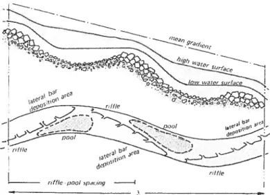
diagram proposed by Leeder [1983] prcsents a general model ofthe interactions bctween the turbulent flow, sedirnent transport, and bed topography from which the bedfornis wc observe emerge (Figure 2.1). Landmark studies from each ofthe three areas are briefly reviewed to present a more general introduction to the formation ofriffle-pools.

2.1.1 Turbulent flou’over u grave!bed

There are two main approaches for describing the flow field: time-indcpendent statistics and tirne-dcpendent definitions ofcohercnt events. The following paragraphs define and review standard distributions ofcommon turbulent flow statistics such as mean velocity, shear stress, and turbulence intensity. For two-dirnensional flows, the streamwise velocity profile is calccilatcd within the boundary layer using the law ofthe wall [Prandtt,

1925]:

11* K k.

Figure 2.1 -Conceptual model of interactions between llow, represented by a rneasured tirne serics

ofinstantaneous velocities; particle movcindnt, represented by individual particles, and

bed brin devcloprncnt, rcpresented by a rifile-pool unit (fromLeeder, 1983).

where Uis the mean downstream velocity, zt is the shear vclocity, Kis the Von-Karman

constant

₍

(2.2)

where p is the fluid dcnsity. The boundaiy layer is dcfined as the region close to a solid surface wherein the surface exerts a drag force on the moving fluid [Henderson, 1966]. A conceptual diagram of the boundary layer is showu in Figure 2.2. The boundary layer can be divided into the iimer or wall region, and the intermediate and the near surface rcgions, collectively referred to as the outer region. Equation 2.1 only applies in the wall region. In the outer region, a wake dcfect parameter can be applicd [Cotes, 1956] such that

U1U

—‘ln--+211-cos--) (2 3)

U _{K k. K 2k}

where U,,,., is the maximum time-averagcd velocity in the water column and FI is Coles’ wake parameter.

A critical question for this study is the effect ofa non-uniforrn boundary on turbulent flow properties. In a series offlume cxpcrimcnts to examine topographically induced deceleration and acceleration over rough surfaces, Kimnoto anci Graf[1995] found that FI varies as a function ofthe parameterfi, which reprcscnts the rate offlow

expansion/constriction:

flrr0o$fi forZ/Y2 (2.4a)

flzrO.0$,B+0.23 forZ/Y> 5 (2.4b)

fi

fi

fi>

effect of/J on flow profiles is shown in Figure 2.3. The profile is ftiller in accelerating fiows so that the highest velocity occurs doser to the bed, whereas decelerating flows are charactcrized by a positive gradient between velocity and depth throughout the flow depth. This change has implications for shcar stress and the generation of turbulence.

7 08 04 02 o 03 05 07 09 11 13

Figure 2.3 -Velocity profiles for uniform and non-uniform llows IKironotoand Graf 1995]

Reynolds shear stresses represent the mornentum flux due to the exchange offluid between layers of fiuid travelling at different velocities. In two-dirnensional uniform flows, this stress eau be represented as

(2.5)

where u and y, are the instantaneous vclocity fluctuations about the mean and the overbar

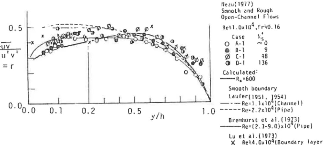
indicates the mean over the length of the velocity series. The behaviour ofthe Reynolds shear stress through the boundary in unifonii flow is sbown for srnooth and rough channet boundaries in Figure 2.4. When normalized by the product of the streamwise and vertical velocity standard deviations to obtain the correlation coefficient (r), the distribution is independant of the properiies ofmean flow and ofroughness [Nezu ami Nakagawa, 1993]. The correlation coefficient reaches a maximum bctwcen 4 and 5 in the intermediate zone and is nearly constant throughout this zone.

C)

u j _÷

Figure 2.2-Conceptuat diagram ofregions in (lieflow field and coordinate system.

.&

decelerating

uniform

-o-

accelerating

$

1h,z( 1977) Soo1h and f1ouh Open—Chantic 1 F1 o.s 0 5 q R1Oiû,l rO.15 — O Culculatea . —R6Qû Se:ooth boundury tàutet(1951 9S4) 0.0 — ——Rel.h1fl Chanci) 0.0 0.1 0.2 0.5 . 1.0 ---R2?e1O1(Ppe) Brcchurst et al. (I 93) Re(2. 3—9.0» lQ’(Pipe) Lu et aL(l973) X Reh3.0x104(Bounduty layer)

figure 2.4—Correlation coefficient of the Reynolds shear stress in uniform flow jNeztt wd

Nakagawa, 19931

Turbulence is generated as a resuit ofthe torque resultant from opposite shear stresses applicd between layers of ftuid moving at different speeds. In uniforrn and 2D flows the rate of turbulence generation (G) can be obtained from the velocity gradient [Nc.ztiaiidNakcigaii’a, 1993]:

G=_t(4L) (2.6)

Measured turbulence intensities are shown for srnooth and rough bcd channels in Figure 2.5. The relations are independent ofroughness except near to thc wall, wherc the normalizcd turbulence intensity is targer over smooth boundaries. Peak turbulence intensitics occur doser to the watt than maximum correlation values.

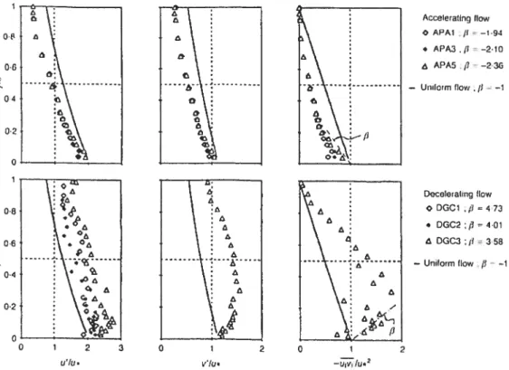
The results of Kironoto auJ Graf[1995] demonstrate the effects ofthe changes to mean velocity profiles in non-unifonvi ftow on turbulence intensities and Reynolds shear stress (figure 2.6). In decelerating flows, the velocity gradient is greater in the outer region compared with uniforrn flows. This increases momentum exchange and turbulence

generation in the outer region, which translates into higher turbulence intensities. In accclerating flows, velocity gradients are rnuch less inthe outer layer, which reduces shear stress and turbulence, espccially when compared to the tremendous shear stresses in the muer layer, wherc a large velocity gradient cxists. These resutts have becn confirmed by subsequcnt studies to clarify spccific aspects ofthe changes to the boundaty layer in

non-9

unifonri flows, but this research area remains active [Songand Graf 1 994; Afzatimehr a17d

Anctil, 1999; Song amiCÏiiew, 20011.

Gr19?I) tL-uu1c) eZu 977) 7Hct-F Ims) Rogi Opn—c

Pon Op,r,—Chon1 7CC

3.0 c-)7O3. FrO.1 _{Obs.rvQd C.rr}

7 uIU. v/U, P] 0 7 e—Thcort1 C,r,e5 ]\\q\

(Z

-u

Figure 2.5-Distribution of turbulence intensities in uniform flow over smooth and rough bcds

‘o

Figure 2.6-Turbulence intensities and normalized Reynolds shear stress distributions in non

uniforin llowtKiro;wto md Graf 1995)

Although prelirninary observations of turbulent structure in rivers [Matthes, 1947] and conceptual model ofwall turbulence [Theodosen, 1952] indicated otherwise, turbulence was long thought to be a ftindamentally stochastic or time-independent phenomenon

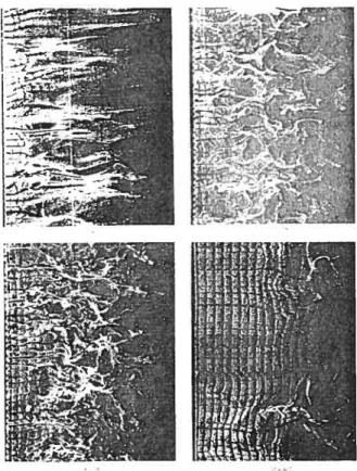
[Heiideeson, 1966]. Ground-breaking work in the 1960s pcmianently changed this vicw. KIIne et cii. [1 967] were the first to demonstrate the occurrence of cohcrent evcnts in the form of streaks and intermittent bursts above a smooth boundary (figure 2.7). Corino anci

Broclkey [1969] subsequently identified a sweep-ejection sequence and conHmied that these evcnts were responsible for the significant part of the momentum exchange betwecn the inner and outer flow regions. Coherent structures are not rcstricted to srnooth wall boundaries. Grass [1971] and Grass andMaiisotw-TeÏwani [1996] found that the sweep ejcction model could be applied to flow over rough boundariesin spitc of the disruption to the boundarv layer. Kfrkbride [1993] demonstrated that the cjections may derive from the separation zones hehind sediment clasts in gravet bed. Coherent structures also occur in the outer region. FaÏco [1977] used the controlled injection ofa fog ofoil droplets to identify cohercnt structures occurring at two scales (Figtire 2.8) At lowReynolds numbers the structure tvas dominated by three-dimensional vortices he called 1typical cddies’. As thc

u,/u* Vlu.

2 1 2