A new proposal for reliable unicast and multicast transport in Delay Tolerant Networks

(1)

HAL Id: hal-00726799

https://hal.archives-ouvertes.fr/hal-00726799

Submitted on 31 Aug 2012

HAL is a multi-disciplinary open access

archive for the deposit and dissemination of

sci-entific research documents, whether they are

pub-lished or not. The documents may come from

teaching and research institutions in France or

abroad, or from public or private research centers.

L’archive ouverte pluridisciplinaire HAL, est

destinée au dépôt et à la diffusion de documents

scientifiques de niveau recherche, publiés ou non,

émanant des établissements d’enseignement et de

recherche français ou étrangers, des laboratoires

publics ou privés.

A new proposal for reliable unicast and multicast

transport in Delay Tolerant Networks

Arshad Ali, Tijani Chahed, Eitan Altman, Manoj Kumar Panda, Lucile

Sassatelli

To cite this version:

Arshad Ali, Tijani Chahed, Eitan Altman, Manoj Kumar Panda, Lucile Sassatelli. A new proposal

for reliable unicast and multicast transport in Delay Tolerant Networks. IEEE International

Sympo-sium on Personal Indoor and Mobile Radio Communications (PIMRC), Sep 2011, Toronto, Canada.

pp.1129-1134, �10.1109/PIMRC.2011.6139673�. �hal-00726799�

(2)

A New Proposal for Reliable Unicast and Multicast

Transport in Delay Tolerant Networks

Arshad Ali, Tijani Chahed

{arshad.ali, tijani.chahed}@it-sudparis.eu Institute Telecom, Telecom SudParis,

UMR CNRS 5157, 9 rue C. Fourier 91011 Evry Cedex, France

Eitan Altman, Manoj Panda

{eitan.altman, manoj.panda}@sophia.inria.fr INRIA, 2004 Route des Lucioles 06902 Sophia-Antipolis, France

Lucile Sassatelli

sassatelli@i3s.unice.fr I3S, University Nice Sophia Antipolis-CNRS UMR 6070

06903 Sophia Antipolis, France

Abstract—We propose a new scheme for reliable transport, both for unicast and multicast flows, in Delay Tolerant Networks (DTNs). Reliability is ensured through the use of Global Selective ACKnowledgements (G-SACKs) which contain detailed (and potentially global) information about the receipt of packets at all the destinations. The motivation for using G-SACKs comes from the observation that one should take the maximum advantage of the contact opportunities which occur quite infrequently in DTNs. We also propose sharing of “packet header space” with G-SACK information and allow for random linear coding at the relay nodes. Our results from extensive simulations of the proposed scheme quantify the gains due to each new feature.

Index Terms—Delay Tolerant Networks (DTNs), reliable trans-port, multicast, network coding

I. INTRODUCTION

Delay Tolerant Networks (DTNs) are Mobile Ad hoc NET-works (MANETs) where the number of mobile nodes per unit area is so small that the connectivity between the nodes is highly intermittent. In a DTN, two nodes can communicate only when they come into contact with each other due to their mobility. Hence, the transport of packets in DTNs is very much dependent on the mobility of the nodes and the packet replication method [1]. TCP turns out to be extremely inefficient for reliable transport in MANETs because it misin-terprets losses due to link failures as losses due to congestion [2]. The situation is even worse in the case of DTNs since connectivity in DTNs is highly intermittent [3].

In this paper, we propose a new reliable transport mech-anism for DTNs which is based on a novel Global Selec-tive ACKnowledgement (G-SACK) scheme. A G-SACK can potentially contain global information about the receipt of packets at each destination in the network. We further propose to put the G-SACK information in the “packet header space” – an enhancement akin to piggybacking. We also allow the use of random linear coding [4] of packets from different sources so as to share the “packet payload space” between packets of different flows in the network.

Literature Survey: Much of the existing literature on DTNs focuses on the routing aspect and few works consider reliable transport. The literature on transport in DTNs is primarily concerned with deep-space communication.

The DTN Bundle Protocol [5] describes the end-to-end exchange of messages (bundles) in DTNs. It specifies a

framework rather than a concrete protocol implementation. The “Saratoga” protocol [6] provides an IP-based convergence layer in DTNs supporting store-and-forward of bundles. It performs UDP-based transfer of IP packets with Selective Negative Acknowledgements (SNACKs). It is more flexible than TCP, although it may not always be reliable. The Licklider Transmission Protocol (LTP) [7] is designed to serve as a DTN convergence layer protocol over long and/or often disconnected links, such as those encountered in the interplanetary networking. It provides retransmission-based reliable transfers over single-hop connections and supports both reliable and unreliable data transmission.

The CFDP protocol [8] provides file copy services over a single link and require all parts of a file to follow the same path to the destination. The Deep-Space Transport Protocol (DS-TP) [9] is based on double automatic retransmission to provide proactive protection against link errors. The level of redundancy introduced by DS-TP affects both the storage space requirement of intermediate DTN nodes and the end-to-end delivery delay of data to its destination. The TP-Planet protocol [10] employs additive increase multiplicative decrease control mechanism and uses time-delayed SACKs to deal with asymmetric bandwidth. The SCPS-TP protocol [11] adopts TCP’s main functionalities and extends them in order to deal with some of the unique characteristics of deep-space links. The open loop rate control part of SCPS-TP makes also use of SNACKs. In [12], four different acknowledgment strategies are considered, namely, hop-by-hop, active receipt, passive receipt and network-bridged receipt. The Delay-Tolerant Transport Protocol (DTTP) is proposed in [13] in order to increase relia-bility and efficiency (in terms of resource utilization) in DTNs. DTTP provides both reliable and unreliable communication with trade-off between reliability and end-to-end delivery delay. Full reliability requires extensive retransmissions, which obviously extends overall transfer time.

In this paper, we ensure reliable transport in DTNs through the use of acknowledgements and coding. Our reliable trans-port mechanism focuses primarily on the ACK mechanism and takes the maximum advantage of intermittent contacts. Organization of the Paper: In Section II, we describe our network setting and the mobility model. In Section III, we propose our reliable transport scheme. In Section IV, we

(3)

explain the different scenarios we consider so as to exhibit the gains brought by each feature of our scheme. In Section V, we provide simulation results with insightful observations. Section VI concludes the paper.

II. NETWORKSETTING

The network consists of N + S mobile nodes. There are S source/sink nodes that act as sources, or destinations or both. There are N relay nodes which do not have any traffic of their own (during the period of time under consideration), but are otherwise identical to the source/sink nodes. In fact, a source/sink node can act as relay for another source/sink node. We allow for both unicast (one source to one destination) and multicast (one source to multiple destinations) sessions. Also, a node can be a destination for multiple sources.

Each source intends to send one packet to its destination(s). Each source-destination pair defines a flow. A multicast flow consists of multiple flows. The source/sink nodes are indexed by 1, . . . , S. The flow matrix A = [aij] is an S × S matrix,

where, ∀i, j = 1, . . . , S, the entry aij= 1if node i intends to

send a packet to node j; otherwise, aij= 0.

Two nodes “meet” when they come within the communi-cation range of each other. We assume that the successive inter-meeting times between any two specific nodes, say i and j 6= i, are i.i.d. exponential random variables with mean 1/β. Our assumption of i.i.d. exponential inter-meeting times is motivated by [14], [15], [16], wherein it was shown via sim-ulations that, for “random waypoint” and “random direction” mobility models, the assumption of i.i.d. exponential inter-meeting times provides extremely accurate approximations for actual inter-meeting times provided that the communication range r L, where L × L denotes the area of the network.

III. OURPROPOSEDRELIABLETRANSPORTSCHEME

Our reliable transport proposal consists of four features: 1) SACKs: Upon receipt of a packet, a destination

gen-erates a Selective ACK (SACK) indicating the set of sources from which it has already received the packet. This is in contrast with an ACK scheme in which only the currently received packet is acknowledged. A SACK can acknowledge multiple sources about the receipt of packets at a specific destination.

2) Updating SACKs to form G-SACKs: As a node carrying the SACK information generated by a des-tination meets with other nodes which possibly carry packet receipt information from other destinations, the information contained in the SACKs is then updated to form G-SACKs. This is in contrast with a SACK scheme in which the SACKs generated by the destinations reach the sources without being updated inside the network. A G-SACK can acknowledge multiple sources about the receipt of packets at multiple destinations.

3) Sharing of the packet header space: The G-SACK information is put in the (transport layer) header. This alleviates the competition between ACK and packet

traffic to get access to relay buffers, and we derive benefits akin to piggybacking.

4) Random linear coding at the relays: Packets are combined to form random linear combinations. This allows packets from different destinations to share the packet payload space, and we derive the benefits of network coding especially with multicast flows. In practice, with time-varying sets of source/sink nodes and with multiple packets flowing between source-destination pairs, each entry for G-SACK information could be im-plemented by the tuple {sourceID, destinationID, packetID, receiptFlag}. The entries could be maintained as a list with an upper limit L to the number of such entries that can be kept in the (transport layer) headers. Clearly, L need not be larger than Lmax := S × S × M, where S denotes the number of

source/sink nodes and M denotes the number of packets per flow. The parameter L can be appropriately chosen to match the average number of flows in the network times the average number of packets per flow.

IV. NETWORKSCENARIOS ANDPERFORMANCEMETRICS

In the following, we consider three example networks each consisting of 4 source/sink nodes:

• Unicast: Each source unicasts its packet to one of the

other S − 1 nodes. The corresponding flow matrix is AU =     0 1 0 0 0 0 1 0 0 0 0 1 1 0 0 0     (UnicastFlowMatrix)

with an average source/destination-degree equal to 1.

• Multicast: Each source multicasts its packet to all the

remaining S − 1 nodes. The flow matrix is given by AM =     0 1 1 1 1 0 1 1 1 1 0 1 1 1 1 0     (MulticastFlowMatrix)

with an average source/destination-degree equal to 3.

• Mixed: Half of the nodes have unicast sessions and the

other half have multicast sessions. The flow matrix is AX=     0 1 1 1 0 0 1 0 1 1 0 1 1 0 0 0     (MixFlowMatrix)

with an average source/destination-degree equal to 2. It is useful to view the G-SACK information as a matrix. The (true) G-SACK matrix B = [bij] is an S × S matrix,

where, ∀i, j = 1, . . . , S, the entry bij = 1if node i has already

received the packet from node j; otherwise, bij= 0. However,

the G-SACK information at a particular relay node might differ from the true G-SACK matrix. For example, even after the packet from node j has already been received at node i (and a corresponding acknowledgment has already been generated), the entry bij of the (local) G-SACK matrix BR at some relay

(4)

node ‘R’ may still be equal to 0 if ‘R’ has not yet come in contact with a node having this information.

When all the packets have been received by their intended destinations, and sufficient mixing has occurred inside the network, the packet receipt information at all the destinations is contained in the G-SACKs. Then, the G-SACK matrix BR

at a relay node ‘R’ is given by AT _{– the transpose of the}

flow matrix A. For example, for the network corresponding to the UnicastFlowMatrix AU, BR = ATU indicates that all the

packets have been received by their destinations, and BR=     0 0 0 0 1 0 0 0 0 1 0 0 0 0 1 0    

indicates that all the packets, except that the packet from 4 to 1, have been received by their destinations. This may happen for two reasons: (i) either 1 has not yet received the packet from 4, (ii) or the acknowledgment for the said packet has not yet been mixed with the above G-SACK inside the network. Clearly, different G-SACKs may contain different information. We set the buffer capacity at the relays to 1 which means that a relay can store at most one packet and/or G-SACK at any time. In reality, a relay could store multiple packets and/or G-SACKs. However, one must also devise an appropriate buffer management policy to: (i) ensure fair access of the buffer space to packets from different flows, and (ii) keep proper balance between “combining packets by coding” and “keeping the packets separate using more buffer space”. Evaluation of such advanced issues is part of our ongoing work. In fact, the buffer capacity (in packets) of any relay would be typically smaller than the number of ongoing flows. Thus, for our example networks with 4 source/sink nodes, a buffer capacity of 1 packet/G-SACK is a reasonable choice.

To quantify the gain due to each individual feature of our proposal, as well as due to the overall scheme, we study the following scenarios:

• Scenario A: The destinations generate plain ACKs.

Pack-ets and ACKs are separate so that a relay can store either an ACK or a packet. There is no coding at the relays.

• Scenario B: The destinations generate SACKs instead of

plain ACKs. Packets and SACKs are separate, as before. There is no coding at the relays.

• Scenario C: The destinations generate SACKs and the

SACKs are updated inside the network to form G-SACKs. Packets and G-SACKs are separate, as before. There is no coding at the relays.

• Scenario D: G-SACKs are put in the packet headers.

There is no coding at the relays.

• Scenario E: G-SACKs are put in the packet headers.

Packet are combined by coding at relays. We next detail the dynamics of each scenario. Scenario A:

1) When relay i, which is empty (i.e., relay i has neither a packet nor an ACK), meets with a source, relay i gets a copy of the packet from the source.

2) When relay i, which is empty, meets with another relay j, j 6= i, which has a packet, relay i gets the packet. 3) When relay j, which has a packet, meets with a

destina-tion (of the packet), the destinadestina-tion gets the packet and the packet in relay j is replaced with an ACK.

4) When relay i, which is empty, meets with another relay j, j 6= i, which has an ACK, relay i gets the ACK. 5) When relay j, which has an ACK, meets with a source

(which needs the ACK), the source receives the ACK. Scenario B: This scenario differs from Scenario A in only one aspect, namely, the destination generates a SACK (instead of an ACK) indicating the set of packets it has successfully received so far.

Scenario C: The destinations generate SACKs upon receiv-ing packets, as in Scenario B. The SACKs are updated with latest information about the receipt of packets each time a relay meets with a destination or with another relay to form G-SACKs.

Scenario D: In this scenario, the G-SACKs share the packet header space. Thus, upon receiving a packet from a relay i, a destination puts its latest packet receipt information into the header of the packet in relay i. Whenever two nodes meet, they update their G-SACK parts. If one of the nodes is empty, the empty node just copies the entire packet (including the G-SACK part) from the other node.

Scenario E: This scenario is similar to scenario D, except that packet payload parts are combined by Random Linear Combination (RLC) over Galois field Fq. When relay j, which

has a pure or a coded packet, meets with a source or with another relay that has a pure or a coded packet, relay j replaces its content with a new coded packet.

Upon receiving a coded packet, a destination checks (using the encoding vector in the coded packet) whether the coded packet is useful for it. A destination accumulates all useful coded packets and tries to extract the pure packet(s) for which it is a destination. When enough independent linear combina-tions have been gathered, a pure packet can be extracted, and the packet receipt information at the destination gets updated and shared with other nodes as in Scenario D.

A. Performance Metrics

We quantify the gain due to each feature in our scheme through the following performance metrics:

• Forward delay: For a unicast (resp. multicast) flow it

refers to the delay between the sending of the first copy of the packet from the source and its receipt at the destination (resp. at all the destinations). For the whole network, it refers to the average of the per-flow delays.

• Round trip delay: For a unicast (resp. multicast) flow

it refers to the delay between the sending of the first copy of the packet from the source and the receipt of the corresponding acknowledgement (resp. acknowledge-ments from all destinations). For the whole network, it refers to the average of the per-flow delays.

• Overall success probability: It refers to the fraction

(5)

0 100 200 300 400 500 0 0.2 0.4 0.6 0.8 1 Time t

Round Trip Delay CDF

All Unicast Sessions

Scenario A Scenario B

Fig. 1. Comparison of round trip delay CDF of scenario A versus scenario B: unicast sessions for all source/destination pairs.

1000 200 300 400 500 0.2 0.4 0.6 0.8 1 Time t

All Multicast Sessions

Fig. 2. Comparison of round trip delay CDF of scenario A versus scenario B: multicast sessions for all source/destination pairs.

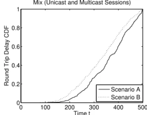
0 100 200 300 400 500 0 0.2 0.4 0.6 0.8 1 Time t

Mix (Unicast and Multicast Sessions)

Fig. 3. Comparison of round trip delay CDF of scenario A versus scenario B: mix of 50% unicast and 50% multicast sessions.

reach(es) the source within the simulation time t. Its computation is similar to that of round trip delays.

V. SIMULATIONRESULTS ANDOBSERVATIONS

We developed a customized simulator in Matlab (codes can be provided on request) for DTNs of the type discussed in Section II. Given the flow matrix, our simulator can simulate any such DTN with options to enable/disable the four features listed in Section III. At present, our simulator simulates an error-free link layer, but it can be adopted to capture the link layer errors (via the variable forwardingProbability available in our simulator).

The simulation setting is as follows: number of relays N = 100, Galois field size q = 2, and mean inter-meeting intensity β = 0.005. We simulate each scenario 1000 times, each run for a duration t = 500 units of time.

A. Benefit of SACK over ACK

In Figures 1, 2 and 3, we compare the Cumulative Distri-bution Functions (CDFs) of the the round trip delay (random variable) in Scenarios A and B for unicast, multicast and 50% mix of unicast and multicast, respectively. We observe that, in Figure 1, the delays in Scenarios A and B are stochastically identical. However, in Figures 2 and 3, the delay CDF with SACKs stays above the delay CDF with ACKs implying that the delay with SACKs is stochastically smaller than the delay with plain ACKs (which is a stronger result than ordering of the mean delays). This is due to the fact a single SACK provides packet receipt information at a specific destination to multiple sources. In our unicast example, each destination is connected with exactly 1 source in the flow matrix, and hence, SACKs are identical to ACKs and there is no improvement. This also explains why the gain due to SACKs increases as the average “source-degree” of the destinations, i.e., the average number of source(s) from which destinations are receiving packet(s), increases from 1 for all unicast sessions (Figure 1) to 2 for 50% mix of unicast and multicast sessions (Figure 3) to 3 for all multicast sessions (Figure 2).

B. Benefit of G-SACK over SACK

In Figures 4, 5 and 6, we compare the round trip delay CDFs in Scenarios B and C for unicast, multicast and 50%

mix of unicast and multicast, respectively. We observe that the delay with G-SACK is stochastically smaller than with SACKs, even for the unicast example. This is due to the fact that, unlike a SACK which carries information from a single destination that generates it, a G-SACK initially generated by a destination gathers packet receipt information from multiple destinations on its way back to the sources. Thus, the number of relays carrying packet receipt information from any specific destination increases inside the network. The improvement in delay performance due to G-SACKs over SACKs increases as the fraction of multicast sessions increases because a multicast session must continue until acknowledgements from all the destinations are received, and the G-SACKs help in this regard. C. Benefit of putting G-SACK in packet headers

In Figures 7, 8 and 9, we compare the round trip delay CDFs in Scenarios C and D for unicast, multicast and 50% mix of unicast and multicast, respectively. We observe that the delay with G-SACKs put in packet headers is stochastically smaller than with use of separate G-SACKs and packets. The observed gain in this case is akin to “piggybacking” which eliminates the competition between the packet and ACK traffic to get access to relay buffers. It is important to observe that the gain in this case decreases as the fraction of multicast sessions increases because piggybacking, which amounts to increase in capacity in our setting, is less beneficial to multicast flows that have more stringent requirements to be considered successful. D. Benefit of coding at relays

In Figures 10, 11 and 12, we compare the forward delay CDFs in Scenarios D and E for unicast, multicast and 50% mix of unicast and multicast, respectively. We choose to quantify the gains based on delays in the forward path because this is where packets are being coded (and the return delays are identical). The benefit of coding indeed shows up in the forward path (Figures 10, 11 and 12). This gain is due to two reasons: (1) the destination need not wait for a specific packet, and (2) packets from different sources share the limited buffer space available at the relays.

(6)

0 100 200 300 400 500 0 0.2 0.4 0.6 0.8 1 Time t

Scenario B Scenario C

Fig. 4. Comparison of round trip delay CDF of scenario B versus scenario C: unicast sessions for all source/destination pairs.

0 100 200 300 400 500 0 0.2 0.4 0.6 0.8 1 Time t

Fig. 5. Comparison of round trip delay CDF of scenario B versus scenario C: multicast sessions for all source/destination pairs.

0 100 200 300 400 500 0 0.2 0.4 0.6 0.8 1 Time t

Fig. 6. Comparison of round trip delay CDF of scenario B versus scenario C: mix of 50% unicast and 50% multicast sessions.

0 100 200 300 400 500 0 0.2 0.4 0.6 0.8 1 Time t

Scenario C Scenario D

Fig. 7. Comparison of round trip delay CDF of scenario C versus scenario D: unicast sessions for all source/destination pairs.

0 100 200 300 400 500 0 0.2 0.4 0.6 0.8 1 Time t

Fig. 8. Comparison of round trip delay CDF of scenario C versus scenario D: multicast sessions for all source/destination pairs.

0 100 200 300 400 500 0 0.2 0.4 0.6 0.8 1 Time t

Fig. 9. Comparison of round trip delay CDF of scenario C versus scenario D: mix of 50% unicast and 50% multicast sessions.

0 50 100 150 200 250 300 0 0.2 0.4 0.6 0.8 1 Time t Forward Delay CDF

Scenario D Scenario E

Fig. 10. Comparison of forward delay CDF of scenario D versus scenario E: unicast sessions for all source/destination pairs.

0 100 200 300 400 500 0 0.2 0.4 0.6 0.8 1 Time t Forward Delay CDF

Fig. 11. Comparison of forward delay CDF of scenario D versus scenario E: multicast sessions for all source/destination pairs.

0 100 200 300 400 500 0 0.2 0.4 0.6 0.8 1 Time t Forward Delay CDF

Fig. 12. Comparison of forward delay CDF of scenario D versus scenario E: mix of 50% unicast and 50% multicast sessions.

E. Overall gain Vs. number of relays

We obtain and compare additional simulation results with N = 125, 150, 200. But, as suggested in [16], we keep the product Nβ as constant. In Figures 13 to 15 and Figures 16 to 18, we compare the average round trip delay and the overall success probability, respectively, in Scenarios A and E for unicast, multicast and 50% mix of unicast and multicast, respectively, by varying the number of relays N. In Figures 13 to 15, each point is calculated by averaging over only those runs in which the acknowledgments have reached within the simulation time (respective success probabilities are shown in

Figures 16 to 18). We also show the 95% confidence intervals (with 1000 runs). Note that the 95% confidence intervals for Scenario E are too narrow to be visible.

The decrease in the mean round trip delay with our over-all scheme as compared to the basic scheme A is indeed remarkable for all values of N = 100, 125, 150, 200. It is also worth noticing that the overall success probability with our proposed scheme is equal to 1 for all values of N = 100, 125, 150, 200. In our simulation experiments (not reported here), we have observed that our proposed scheme can achieve an overall success probability of 1 even when the

(7)

100 120 140 160 180 200 0 50 100 150 200 250 300 350

Number of Relay Nodes (N)

Mean Round Trip Delay

ScenarioA ScenarioE

Fig. 13. Comparing round trip delay of Sce-nario E with SceSce-nario A: unicast sessions for all source/destination pairs. 100 120 140 160 180 200 0 100 200 300 400 500

ScenarioA Scenario E

Fig. 14. Comparing round trip delay of Sce-nario E with SceSce-nario A: multicast sessions for all source/destination pairs.

100 120 140 160 180 200 0 50 100 150 200 250 300 350 400

ScenarioA Scenario E

Fig. 15. Comparing round trip delay of Sce-nario E with SceSce-nario A: mix of 50% unicast and 50% multicast sessions.

100 120 140 160 180 200 0.65 0.7 0.75 0.8 0.85 0.9 0.95 1

Success Probability

Scenario A Scenario E

Fig. 16. Comparing Overall Success probability of Scenario E with Scenario A: unicast sessions for all source/destination pairs.

100 120 140 160 180 200 0.2 0.3 0.4 0.5 0.6 0.7 0.8 0.9 1

Success Probability

Fig. 17. Comparing Overall Success proba-bility of Scenario E with Scenario A: multicast sessions for all source/destination pairs.

100 120 140 160 180 200 0.4 0.5 0.6 0.7 0.8 0.9 1

Success Probability

Fig. 18. Comparing Overall Success probability of Scenario E with Scenario A: mix of 50% unicast and 50% multicast sessions.

number of source/destination nodes is as high as 20 and the number of relays as low as 100.

VI. CONCLUSION

In this paper, we proposed and studied via extensive simu-lations a new proposal for reliable transport in DTNs covering both unicast and multicast flows. Reliability is based on the use of so-called G-SACKs that can potentially contain global information on receipt of packets at all destinations.

We further allowed for the sharing of the packet header space with G-SACKs to alleviate the competition between ACK and packet traffic and derive benifits akin to piggyback-ing. We also enabled random linear coding at relays so that packets can reach the destination faster. We quantified the gains achieved due to each feature of our proposal as well as the overall gain achieved by all of them.

A more complete evaluation with multiple packet buffers and multiple packet transfers between source-destination pairs is part of our ongoing work.

REFERENCES

[1] S. Biswas and R. Morris, “ExOR: Opportunistic Multi-Hop Routing for Wireless Networks,” in Sigcomm, 2005.

[2] G. Holland and N. Vaidya, “Analysis of TCP Performance Over Mobile Ad Hoc Networks,” ACM Wireless Networks, vol. 8, no. 2, pp. 275–288, March 2002.

[3] M. Ramadas, S. Burleigh, and S. Farrell, “Licklider Transmission Protocol - Motivation,” in RFC-5325, September 2008.

[4] D. Lucani, M. Stojanovic, and M. M´edard, “Random Linear Network Coding for Time Division Duplexing: When to Stop Talking and Start Listening,” in Infocom, April 2009.

[5] K. Scott and S. Burleigh, “Bundle Protocol Specification,” in RFC-5050, November 2007.

[6] L. Wood, J. McKim, W. Eddy, W. Ivancic, and C. Jackson, “Saratoga: A Scalable File Transfer Protocol,” November 13, 2009.

[7] M. Ramadas, S. Burleigh, and S. Farrell, “Licklider Transmission Protocol Specification,” in RFC-5326, September 2008.

[8] CCSDS, “CCSDS File Delivery Protocol (CFDP),” in CCSDS

727.0-B-4, Blue Book, January 2007.

[9] G. Papastergiou, I. Psaras, and V. Tsaoussidis, “Deep-Space Transport Protocol: A Novel Transport Scheme for Space DTNs,” Computer

Communications, Special Issue of Computer Communicationson Delay and Disruption Tolerant Networking, vol. 32, no. 16, p. 17571767,

October 2009.

[10] O. B. Akan, J. Fang, and I. F. Akyildiz, “TP-Planet: A Reliable Transport Protocol for InterPlanetary Internet,” IEEE Journal on Selected Areas

in Communications(JSAC), vol. 22, no. 2, pp. 348–361, 2004.

[11] C. C. for Space Data Systems, “Space Communications Protocol Stan-dards (SCPS) - Transport Protocol (SCPS-TP),” in CCSDS 714.0-B-2,

Blue Book, October 2006.

[12] K. A. Harras and K. C. Almeroth, “Transport Layer Issues in Delay Tolerant Mobile Networks,” in IFIP NETWORKING, 2006.

[13] C. Samaras and V. Tsaoussidis, “DTTP: A Delay-Tolerant Transport Protocol for Space Internetworks,” in ERCIM, 2008.

[14] R. Groenvelt, P. Nain, and G. Koole, “The Message Delay in Mobile Ad Hoc Networks,” Performance Evaluation, vol. 62, pp. 210–228, 2005. [15] M. Ibrahim, A. A. Hanbali, and P. Nain, “Delay and Resource Analysis

in MANETs in Presence of Throwboxes,” Performance Evaluation, vol. 24, no. 9–12, pp. 933–945, October 2007.

[16] X. Zhang, G. Neglia, J. Kurose, and D. Towsley, “Performance Modeling of Epidemic Routing,” Computer Networks, vol. 51, pp. 2867–2891, 2007.