HAL Id: hal-01620034
https://hal.archives-ouvertes.fr/hal-01620034
Submitted on 25 Oct 2017
HAL is a multi-disciplinary open access
archive for the deposit and dissemination of
sci-entific research documents, whether they are
pub-lished or not. The documents may come from
teaching and research institutions in France or
abroad, or from public or private research centers.
L’archive ouverte pluridisciplinaire HAL, est
destinée au dépôt et à la diffusion de documents
scientifiques de niveau recherche, publiés ou non,
émanant des établissements d’enseignement et de
recherche français ou étrangers, des laboratoires
publics ou privés.
Shortcut in DIC error assessment induced by image
interpolation used for subpixel shifting
Michel Bornert, Pascal Doumalin, Jean-Christophe Dupré, Christophe
Poilâne, Laurent Robert, Evelyne Toussaint, Bertrand Wattrisse
To cite this version:
Michel Bornert, Pascal Doumalin, Jean-Christophe Dupré, Christophe Poilâne, Laurent Robert, et
al.. Shortcut in DIC error assessment induced by image interpolation used for subpixel shifting.
Optics and Lasers in Engineering, Elsevier, 2017, 91, pp.124-133. �10.1016/j.optlaseng.2016.11.014�.
�hal-01620034�
Shortcut
in DIC error assessment induced by image interpolation used for
subpixel
shifting
☆
Michel
Bornert
a,
Pascal Doumalin
b,⁎,
Jean-Christophe Dupré
b,
Christophe Poilane
c,
Laurent
Robert
d,
Evelyne Toussaint
e,
Bertrand Wattrisse
fa Laboratoire Navier, UMR 8205, École des Ponts, IFSTTAR, CNRS, Université Paris-Est, Champs-sur-Marne, France b Institut P’, UPR 3346 CNRS, Université de Poitiers, SP2MI, Futuroscope Chasseneuil, France
c CIMAP, UMR 6252, CNRS, CEA, Université de Caen Basse-Normandie, ENSICAEN, Caen, France
d Université de Toulouse; Mines Albi, INSA, UPS, ISAE; ICA (Institut Clément Ader), Campus Jarlard, F-81013 Albi Cedex 09, France eInstitut Pascal, UMR6602, CNRS, Université Blaise Pascal – IFMA, Aubière, France
fLaboratoire de Mécanique et Génie Civil, UMR CNRS 5508, Université Montpellier 2, Montpellier, France
Keywords:
Digital Image Correlation; Uncertainty quantification; Synthetic images; Interpolation; Error assessment
In order to characterize errors of Digital Image Correlation (DIC) algorithms, sets of virtual images are often generated from a reference image by in-plane sub-pixel translations. This leads to the determination of the well-known S-shaped bias error curves and their corresponding random error curves. As images are usually shifted by using interpolation schemes similar to those used in DIC algorithms, the question of the possible bias in the quantification of measurement uncertainties of DIC softwares is raised and constitutes the main problematic of this paper. In this collaborative work, synthetic numerically shifted images are built from two methods: one based on interpolations of the reference image and the other based on the transformation of an analytic texture function. Images are analyzed using an in-house subset-based DIC software and results are compared and discussed. The effect of image noise is also highlighted. The main result is that the a priori choices to numerically shift the reference image modify DIC results and may lead to wrong conclusions in terms of DIC error assessment.
1. Introduction
Digital Image Correlation (DIC) is an advanced experimental full-field measurement technique, which was first proposed in solid mechanics in the 80 s by Peters and Ranson[1]. The basic principle of DIC consists in matching speckle patterns in grey level images of a sample in some reference configuration and several deformed states, assuming convection of the grey level distribution during the transfor-mation. The metrological assessment of such pattern matching proce-dures remains of high interest, as there is still no normalization or adapted procedure validated by the community of users.
One way to characterize, at least partly, metrological performances of DIC is to experimentally generate displacementfields with precisely prescribed displacements or strains[2–8]. In practice, this approach is difficult (or even impossible) to implement because the actual value of the prescribed displacement field to be used as a reference for DIC measurements is often difficult to reach or to control precisely. In addition, it is often complex to separate the various error sources. Even for the simplest case of in-plane uniform sub-pixel image shifting, large
difficulties arise with the classical translation experiment because of positioning errors, optical aberrations, stage imperfections, encoder errors, misalignments, motion drift, etc[6,9]. Obviously the associated errors can alter the DIC error evaluation.
An alternative way is to test DIC in situations for which displace-mentfields are numerically imposed between a reference and some transformed images. Thefirst question is to get a digital un-deformed image that best reflects an image obtained in real imaging conditions, i.e. obtained with classical spray painting, for instance. The most natural way is undoubtedly to capture a real speckle pattern of a given specimen using a digital camera[4,10–16]or using an imaging device dedicated to the sample observation (scanning electron microscope for instance) whose accuracy has to be assessed [15–20]. The main advantage of this approach is to allow the characterization of the measurement errors using the most realistic images with exact speckle characteristics in terms of size, grey level histograms and gradients, as induced by the actual imaging conditions of the experiment: actual contrast on the sample, lighting conditions, actual performance of the used optics. However, this image may also include some unquantified
☆On behalf of the Workgroup“Metrology” of the French CNRS research network 2519 “Mesures de champs et identification en mécanique des solides/Full-field measurements and
identification in solid mechanics”. URL: http://www.gdr2519.cnrs.fr.
⁎Corresponding author.
results are then analyzed in relation to the considered input images (interpolation scheme used to shift the images, direction of displace-ment searched by DIC). In the third part, results are discussed for several image shifting schemes and for noisy images.
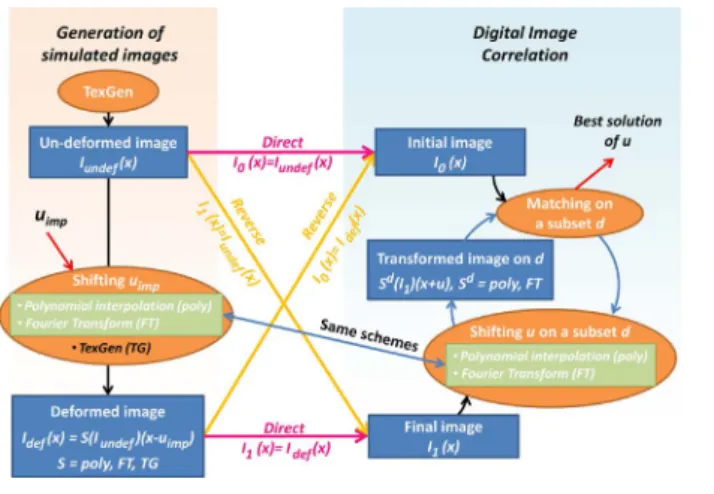
2. Methodology
This section presents the methodology and the tools used for this work (Fig. 1). TexGen software[23]which mimics a texture function is used to generate an un-deformed image. Several sets of shifted images are built from the un-deformed image by using three shifting schemes: polynomial interpolation, Fourier transform and TexGen software, which makes use of the third shifting method. The DIC errors obtained with the set obtained by TexGen software will be compared to those obtained with the other sets obtained with either polynomial interpola-tion or Fourier transform.
2.1. Undeformed image generation
The un-deformed synthetic image, named Iundef, is obtained using
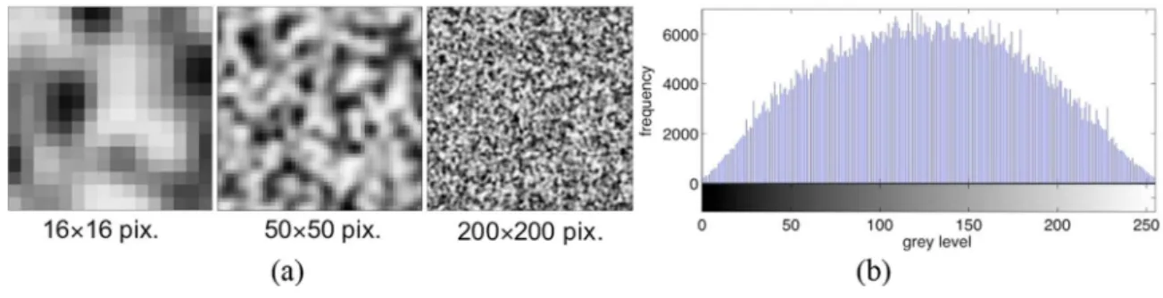
TexGen software[23], as for results presented in[24,25]. This software was designed to be a virtual imaging system that imitates a camera: it implements photometric mapping and digitization of a continuous speckle function based on a modified Perlin noise in the real space, assuming here a 100% fill factor. The integration of each pixel is performed by an oversampling technique. A Gaussian noise with zero-mean and prescribed standard deviation Sncan be added to images,
with an intensityfixed to Sn=2, 4, 8 or 16 grey levels, in order to
account for the effect of image noise. When no noise is superimposed to images, the only image noise to be considered corresponds to the quantization errors, images being coded on 8 bits. In this work, Iundef
image has a size equal to 1024×1024 pixels. Fig. 2 shows several zooms of this image and its grey level histogram.
2.2. Shifted image generation
From the Iundefimage, shifted images, named Idef, are obtained by
three different ways symbolized by a shifting function named S (Fig. 1): (i) Interpolation of Iundefusing several schemes: bilinear or bicubic
interpolation, cubic spline interpolation (S=poly);
(ii) Transformation of the un-deformed image by shifting the signal in Fourier space as shown in[11](S=FT);
(iii) Use of TexGen software, based on an analytically known speckle texture function corresponding to the un-deformed image. This function can be translated, then mapped and sampled to give the translated images that are referred to as“TexGen images” in the following (S=TG).
Fig. 1. Methodology.
or random features which will be hard to reproduce in a realistic way; these ones include image noise (digitization, read-out noise, black current noise, photon noise), under or over sampling because of an imperfect CCD fill factor of the camera sensor, as well as optical imperfections such as distortion. Another solution is to numerically generate the image. This way, most of the image characteristics can be prescribed by the user (e.g. image noise, speckle size, but possibly also image imperfections, etc.) [7,17,21–29]. To generate speckle painting representative contrasts, methods based on the construction of a continuous speckle pattern in 2D space from the random spatial distribution of individual Gaussian marks or from the definition of a continuous luminance field based on a modified Perlin noise function have been proposed. The speckle image is then generated by a photometric mapping and the luminance function defining the marks is digitized on a regular grid corresponding to each pixel of the image, with integration procedures designed to mimic a real image sensor.
The second question is to shift the un-deformed image by a specified displacement field. The generation of the transformed images is usually realized by considering one of the three methods described hereafter. The first method consists in interpolating the un-deformed image. It allows us to create numerically shifted images for any type of image (real or computer-generated). It can be performed in direct space using polynomial, spline or other interpolation schemes [14,15,30,31] or in Fourier space [10,12,32,33]. If interpolation in direct space is used, any
kind of strain field can be produced while with the Fourier method only limited image transformations are possible (translation, dilation, mod-ulation). The second shifting method is based on oversampling of the undeformed image and on generation of reference and deformed image by pixel averaging (binning process). An integer-pixel displacement in oversampled images corresponds to a subpixel displacement after binning. This method can be applied to real and synthetic images. For example, it has been applied by Doumalin et al. [17] for synthetic images of grids tracked by DIC, or more recently by Reu [9] and by Barranger et al. [7]. The third method applies only to speckle fields
generated from a continuous luminance field. As the texture is a mathematical function expressed in real space, any transformation can be applied assuming convection of image intensity [23] and the deformed texture is digitized with exactly the same principles as the reference one.
The different methods presented here allow us to obtain sets of images and to assess DIC displacement field measurement accuracy. For that purpose, the most common analysis consists in considering uniform in-plane sub-pixel image translations. This allows constructing the so-called S-shaped bias error curve and their associated random error curve [11,21,25,32,33], whose characteristics and amplitude depend
on image properties and on both chosen DIC formulation and para-meters. It has been shown in Bornert et al. [24] that this error regime only corresponds to the “ultimate error regime” reached when the chosen subset shape function best fits the actual displacement field. This ultimate error regime has recently been studied through a collaborative benchmark, using synthetic images for which uniform in-plane sub-pixel translations were imposed [25].
To assess DIC performances, the metrological properties of the image matching should not depend on the chosen algorithm to obtain the sets of images, but only on the image characteristics and on the DIC algorithm under use (formulation and associated parameters). The objective of the collaborative work presented in this paper is to study whether image shifting by interpolation introduces some biases in the assessment of errors, in particular when the same interpolation scheme is used in the DIC analysis. The paper is composed of three parts. The first one presents the methodology developed to achieve the goal: description of the way to generate the un-deformed image and the sets of shifted images, of the features of used DIC algorithms, and of the process to determine bias and random errors. The second part deals with results in DIC errors analysis when the same scheme is used to obtain shifted images and to shift the subsets in the DIC process. These
For the three cases, the imposed displacement, named uimp, varies
from 0 to 1 pixel with a step of 0.02 pixel. Note that Iundef(x) and
Idef(x) are the grey levels of the un-deformed image and the shifted
image at integer positions x respectively. As Idef is the Iundefimage
shifted by uimp, the grey level Idef(x) is equal to the grey level
calculated by S at non-integer position (x-uimp) (Idef(x) = S(Iundef)
(x-uimp)). The shifted images are obtained from the un-deformed image
without noise. For the analysis of the effect of noise, the latter is added to each shifted image and to the un-deformed image before application of DIC algorithms.
2.3. DIC algorithms
Sets of images are then analyzed using an ad hoc homemade subset-based DIC software. It allows us to select, if wanted, exactly the same interpolation scheme as the one used to generate the shifted images Idef
(Fig. 1) A new shifting function named Sd which corresponds to
polynomial interpolation (Sd=poly) or Fourier schemes (Sd=FT) on a DIC subset with a size d, is introduced. The software is based on a Newton-scheme minimization of the classical Sum of Squared Difference (SSD) criterion with a zero-order subset shape function (Eq.(1)):
∫
u I x S I x u dS SSD( ) = ( ( ) − ( )( + )) d d 0 1 2 (1) I0(x) and I1(x) are respectively the grey levels of the initial andfinal images used for the DIC computation at integer positions x and
Sd( )( + )I x u
1 the grey levels interpolated for non-integer positions (x
+u).
Subset size d is set to 16×16 pixels. Polynomial interpolation of grey levels is obtained by bilinear or bi-cubic interpolation, bi-cubic spline interpolation. All cases are studied in the paper.
2.4. Error calculation
The methodology to evaluate DIC errors is based on a statistical analysis of n subsets. Measured displacements uiare evaluated for all
positions of a regular square grid in the initial image I0, with a pitch of
16 pixels such that subsets at adjacent positions do not overlap, ensuring the statistical independence of the corresponding errors. The subsets near to image edges are excluded to eliminate measurement artifacts linked to boundaries (n=3844). The displacement error for a subset i is defined by:
Δui=ui−uimp (2)
whereuimpis the imposed displacement.
The standard deviationσu(random error) and the arithmetic mean
(bias error) are calculated with the n subsets[24,25]. 2.5. Studied cases
Table 1summarizes the cases studied with the different shifting methods (polynomial interpolation, Fourier or TexGen), the added
noise level and the“direction” of the material transformation searched for DIC. For this latter parameter, we studied both the direct transfor-mation (from I0=Iundefto I1=Idef) and the reverse one (from I0=Idef
to I1=Iundef). These combinations are studied to evaluate their level of
influence on the evolution of the bias and random errors. It is noted that in most papers on DIC errors assessment based on virtual image shifting, the sole“direct” method is considered.
3. Results
This section is devoted to the presentation of results corresponding to the use of the same scheme to obtain both shifted images and shifted subsets in the DIC process, i. e. studied cases presented in the fourfirst lines ofTable 1(grey area).
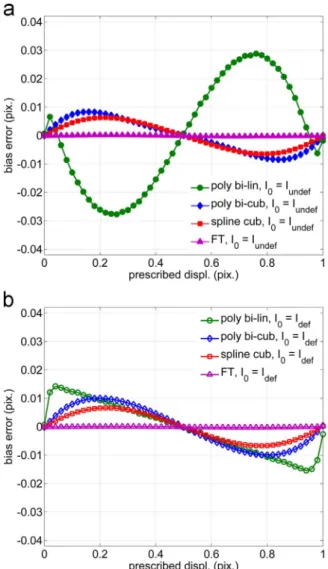
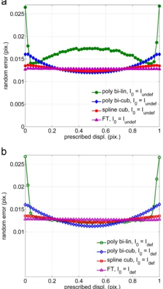
Fig. 3a and b present the bias errors and the random errors versus prescribed displacements, respectively, for various interpolation schemes and for the direct transformation.Fig. 4a and b present the same results considering the reverse transformation. Thumbnails in
Fig. 2. Synthetic un-deformed image: (a) Sub-images, (b) grey level histogram.
Table 1
Studied cases, direct transformation =(I0= Iundef, I1= Idef) and reverse
transforma-tion =(I0= Idef, I1= Iundef).
Iundef S: Shifting Methods for Idef Added Noise (grey levels) Sd: DIC Shifting Methods Transformation
TexGen Bi-linear 0, 2, 4, 8 or 16 Bi-linear Direct Reverse Bi-cubic 0, 2, 4, 8 or 16 Bi-cubic Direct
Reverse Bi-cubic spline 0, 2, 4, 8 or 16 Bi-cubic spline Direct
Reverse Fourier 0, 2, 4, 8 or 16 Fourier Direct
Reverse
Fourier 0 Bi-linear Direct
Reverse
Fourier 0 Bi-cubic Direct
Reverse
Fourier 0 Bi-cubic spline Direct
Reverse TexGen 0, 2, 4, 8 or 16 Bi-linear Direct
Reverse TexGen 0, 2, 4, 8 or 16 Bi-cubic Direct
Reverse TexGen 0, 2, 4, 8 or 16 Bi-cubic spline Direct
Reverse TexGen 0, 2, 4, 8 or 16 Fourier Direct
plots of Fig. 4 present the same results in a scale similar to that of
Fig. 3a and b in order to facilitate comparisons.
As expected for an isotropic texture, all bias curves are central-symmetric with respect to the point (0.5, 0) and all random error curves are symmetric with respect to the vertical median axis corresponding to x=0.5. Indeed an image translation with a shift u smaller than 0.5 pixel and with an error Δu, is equivalent to the image translation with a shift –u, with an error −Δu, deduced by a central symmetry. Such a symmetric image is statistically equivalent to the initial image for such a texture. In addition, the translation –u is itself equivalent to the translation 1-u regarding the one-pixel periodicity of DIC errors
[11,25]. Bias errors for displacements u and 1-u are thus opposite and random errors are equal, provided the set of measurement points considered for the statistical analysis is representative. Because bias curves have an S-shape evolution, the amplitude AΔudefined as the gap
between maximum and minimum error over all imposed displacements allows us to compare bias errors for the different cases. Concerning the random error, evolutions can be very different. Studied cases are then compared using the highest values σmax of the standard deviation
curves. All these values are summarized inTable 2. 3.1. Direct and reverse transformation effect
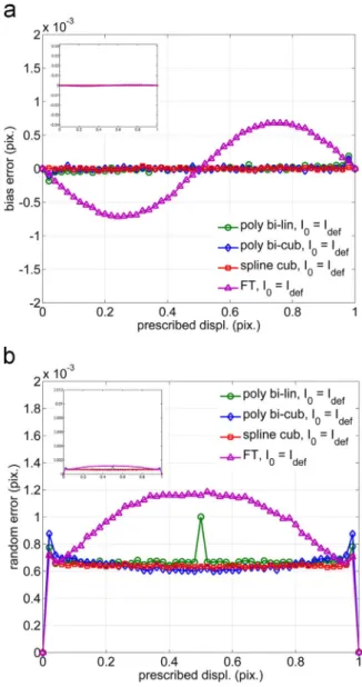
The well-known‘S-shape’ for bias error curves and ‘bell-shape’ for
random error curves presented inFig. 3a and b for direct transforma-tion are in accordance with literature. Different amplitudes depend on the interpolation scheme used to generate and process images. For the bias error (Fig. 3a), amplitudes range from 8.0×10−2pixel for bi-linear polynomial interpolation, 6.3×10−3 pixel for bi-cubic polynomial interpolation, 1.4×10−3 pixel for Fourier transform (noted TF in figures), to 1.1×10−3 pixel for bi-cubic spline interpolation (see
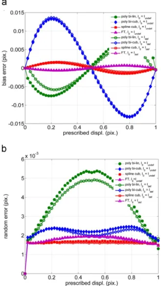
Table 2). For the random error (Fig. 3b), the maximal value also depends on the DIC interpolation scheme. The amplitude of the maxima evolves from about 1.1×10−2 pixel for bi-linear polynomial, 3.4×10−3pixel for bi-cubic polynomial, to about 2.0×10−3pixel for Fourier transform and for bi-cubic spline. Considering the reverse transformation (Fig. 4a and b), it appears that an almost null bias value is always observed, except for the Fourier interpolation (Fig. 4a). The possible observed gap around the null bias may result from computation errors in the correlation criterion minimization. This important observation shows that a misinterpretation can be done when one assesses DIC errors by such a way. The explanation is linked to the use of interpolation scheme. It is presented in next section.
Fig. 3. Bias (a) and random (b) errors for direct transformations, for various interpolation
schemes used for both DIC analysis and image shifting (non-noisy images). Fig. 4. Bias (a) and random (b) errors for reverse transformations, for various interpola-tion schemes used for both DIC analysis and image shifting. Thumbnails present the results in the same scale as in plots inFig. 3(non-noisy images).
3.2. Polynomial interpolation case
To explain the trends previously observed, we choose to show the calculation of SSD criterion from unidirectional grey level profiles and a bilinear polynomial scheme as plottedFigs. 5 and 6.Fig. 5a represents Iundef(x) the grey levels of pixels at integer positions x (blue diamonds)
and S(Iundef)(x) the interpolated grey level profile for real values of x
(blue curve). From these data, S(Iundef)(x-uimp) (red circles) is
calculated. It allows to determine Idef(x) the grey levels pixels at
integer positions x (red circles) inFig. 5b. Note thatFig. 5a and b are shifted by uimpin order to best compare both grey level profiles with
the naked eye.
Considering the reverse transformation (Fig. 5b and c), one has
I x0( ) =Idef( )x and I x1( )=Iundef( )x. Solving Eq. (1)needs to interpolate
grey levels of I1 (blue diamonds) on d (white zone). These values Sd( )( ) =I x Sd(I )( )x
undef
1 are represented inFig. 5c by a blue line. Values Sd( )( + ) =I x u Sd(I )( + )x u
undef
1 are deduced at non integer values x+u.
When interpolation scheme is the same for both transformed images and DIC computation (S=Sd), SSD difference writes as:
S I(undef)( −x uimp) −S I(undef)( + )x u. The optimum of the SSD criterion
also corresponds to u= −uimp and therefore leads to a null error.
Indeed, Fig. 5c shows that grey levels I x0( ) (red circles) and
Sd(I )( −x u )
undef imp (dark-blue dots) are equal. Note that the grey level
profile I x0( ), shifted by uimp, is plotted inFig. 5c (red dashed line) and
superimposed on I x1( ).
Fig. 4shows weak errors different from zero due to quantification
noise, which is not taken into account in the previous reasoning, and that acts in DIC optimization process and does not allow achieving the theoretical optimal displacement. The explanation presented here in a particular case of linear interpolation stays valid for other polynomial
interpolation schemes.
In the case of the direct transformation (Fig. 6a and b), Fig. 6a represents I x0( ) =Iundef( )x the grey levels of pixels at integer positions x
(blue diamonds) and S(Iundef)(x) the interpolated grey level profile for
real values of x (blue curve). From these data and as inFig. 5a, S(Iundef)
(x-uimp) (red circles) can be calculated. It allows to calculate Idef(x)
(red circles) in Fig. 6b. Then I1(x)= Idef(x) is also interpolated to
calculate S Id( )( + ) =x u Sd(I )( + )x u
def
1 at the non-integer positions x+u. Consequently, the both shifting functions S and Sdaccount to evaluate S Id( )( + )x u
1 and grey level differences between Iundef( )x (blue
diamonds) and S S Id( ( )( −x u ))( + )x u
undef imp (red diamonds) appear, as
illustrated in grey level profiles presented inFig. 6b for the optimal of the SSD criterion which corresponds tou=uimp. As inFig. 5c, the grey
level profile I x0( ), shifted by -uimp, is superimposed on the profile I x1( )
(blue dashed line) inFig. 6b. These differences also exist with the other
polynomial interpolation schemes but they are smaller because they introduce curvatures that lead to closer profiles.
Considering the random error curves for reverse transformation for all interpolation schemes (see Fig. 4b and Table 2 except Fourier transform), the main observation is that the maximum of random error is generally smaller than for direct transformation and is almost independent of the prescribed sub-pixel displacement. A mean value of about 0.7×10−3pixel is observed. Following the work by Roux and Hild[13], this value can be linked to the standard deviation of the actual image noise Sn, the average of the squared grey level gradient
I
∇2 of the image, and the subset size d considered in this work,
according to: σ S d I ∝ ∇ u th n 2 (3)
Iundef S: Shifting Methods for
Idef
Added Noise (grey levels)
Sd: DIC Shifting
Methods
Transformation Bias amplitudeAΔu×10−3 Random error maximum
σmax×10−3
TexGen Bi-linear 0 Bi-linear Direct 80 11
Reverse ≈ 0 1
Bi-cubic 0 Bi-cubic Direct 6.3 3.4
Reverse ≈ 0 0.9
Bi-cubic spline 0 Bi-cubic spline Direct 1.1 2
Reverse ≈ 0 0.7
Fourier 0 Fourier Direct 1.4 2
Reverse 1.3 1.2
Fourier 0 Bi-linear Direct 15 5.4
Reverse 12 4.9
Fourier 0 Bi-cubic Direct 26 2.5
Reverse 27 2.4
Fourier 0 Bi- cubic spline Direct 3.0 1.7
Reverse 2.7 1.6
Fourier 0 Fourier Direct 1.4 2
Deverse 1.3 2
TexGen 0 Bi-linear Direct 16 4.6
Reverse 17 5.6
TexGen 0 Bi-cubic Direct 26 2.7
Reverse 24 3
TexGen 0 Bi-cubic spline Direct 2.9 1.8
Reverse 0.9 2
TexGen 0 Fourier Direct 2.5 2.2
Reverse 2.9 2.1
Table 2
I
∇ 2can be evaluated from these images to be 30 grey levels per pixel.
With d =16 pixels, a value of σu th
=0.7×10−3 pixel is found for Sn
=0.35 grey levels (in the case of quantification noise), which gives a good order of magnitude of the image noise due to image quantization
[25].
3.3. Fourier transform case
Concerning Fourier transform (S=FT and Sd=FT), curves are almost the same for both directions of the transformation (see
Table 2, Figs. 3 and 4). Indeed, if the signal, Iundef( )x
R
for x real, is well discretized (regarding Shannon's criterion), the shifting by Fourier transform does not change the signal. In that case, one can consider
S I(undefR )( ) =x IundefR ( )x for each x and for Sd as well. Then the SSD
difference can be expressed as IundefR ( )−x IundefR ( +x u−uimp) and
IundefR ( −x uimp)−IundefR ( + )x u for both direct and reverse transformations,
respectively. At the optimum of the SSD criterion for both ways (i.e.u≈uimp (direct) and u≈ −uimp (reverse)), the difference has the
same expression Iundef( )−X I ( )X
R
undef R
with X≈x (direct) or X≈x−uimp
(reverse). Consequently, in this specific case, bias and standard devia-tion results should in principle be null and not be influenced by the direction of transformation. A slight effect is however observed as a consequence of two facts described hereafter. First, the generated un-deformed images are not periodic, so that the shifting theorem does not rigorously apply for the generation of the deformed image (high
frequencies associated with discontinuities at image boundaries are not well reproduced). Second, Fourier shifting in the DIC algorithms is applied on subsets (which by the way also are non-periodic) much smaller than the whole image so that the resulting interpolation differs from the one used to generate the deformed image. This leads to errors slightly higher for the Fourier approach when analyzing the reverse transformation than for the other interpolation schemes, which are more local and work in exactly the same manner in the DIC and the image generation processes. Note that the presented FT results are obtained with Fourier transform shifting in the DIC process performed with twice the subset size d to limit edge effect and frequency filtering due to small size d. True FT based DIC algorithms, in which interpola-tion is implicitly performed on windows with size d, would probably have led to slightly larger errors.
4. Discussion
The preceding results show that it is possible to conclude in a wrong way about error assessment in DIC. We suppose that it occurs when image polynomial interpolation scheme used for DIC is exactly the same as the one used to generate the shifted images (S=Sd=poly). To discuss
these results, we analyze the DIC errors when shifted images are obtained without interpolation scheme (S‡poly). Two methods are tested in this section: TexGen software (seeSection 2.1) (S=TG), and Fourier transform (S=FT) which is a method usually used for DIC studies in literature [11,13,32]. The discussion will lead first from noiseless images then from noisy images.
4.1. TexGen shifted images
Wefirst focus on quantifications of DIC errors obtained when both Idef and (obviously) Iundef are non-noisy TexGen images (S=TG).
Fig. 7a and b present the curves corresponding to bias and random errors versus the prescribed sub-pixel displacement, for various inter-polation strategies of the DIC software (same symbols as inFigs. 3 and 4
are used), respectively. Both direct and reverse transformations are
Fig. 5. Matching example of 1D grey level profiles for linear interpolation, reverse transform and u= −uimp= −0. 3pixel: (a) Iundef(b) I0and (c) I1,I0: dark-blue dots in red
circles. (For interpretation of the references to color in thisfigure legend, the reader is referred to the web version of this article.)
Fig. 6. Matching example of 1D grey level profiles for linear interpolation, direct transform and u=uimp= 0. 3pixel: (a) I0(b) I1,I0: gaps between blue diamonds and
red diamonds. (For interpretation of the references to color in thisfigure legend, the reader is referred to the web version of this article.)
considered in thesefigures. The error amplitudes are summarized, for all studied situations, in Table 2 (last four lines). Bias and random errors are always present and curves are similar for both transforma-tions. For a given DIC interpolation scheme Sd, the small differences between both transformations can be attributed to statistical conver-gence effects.
Bias error amplitude depends on the interpolation scheme (Sd=poly, FT) used in the DIC software (see Fig. 7a). As already reported in[11], spline interpolation diminishes this bias amplitude in comparison to other polynomial interpolation schemes and gives the same order as for Fourier transform: it is about 2.6×10−2pixel for bi-cubic polynomial, 1.6×10−2pixel for bi-linear polynomial, 2.9×10−3 pixel for bi-cubic spline interpolations and 2.5×10−3pixel for Fourier transform. The sign of this bias error depends on the interpolation used. In contrast to curves obtained inSection 3, bias error curves for direct transformation are similar but amplitudes are smaller. Indeed, when using TexGen shifting (S=TG), polynomial interpolation is used once only in DIC process contrary to interpolation shifting process for which interpolation is also used to create shifted images (S=Sd=poly).
When reverse transform is considered, errors are higher with TexGen (S=TG, Sd=poly) than with polynomial interpolation shifting (S=Sd=poly).
Let us now focus on random errors obtained in the same conditions. They are presented inFig. 7b. These errors versus prescribed displace-ment present‘bell-shaped’ curves with one or two maxima depending on the DIC interpolation scheme. The amplitude of the maxima
Fig. 7. Bias (a) and random (b) errors evaluated when considering pairs of TexGen images, for both direct (-•-) and reverse (-○-) transformations (non-noisy images).
Fig. 8. Bias (a) and random (b) errors evaluated when considering pairs of Fourier-shifted images, for both direct (-•-) and reverse (-○-) transformations (non-noisy images).
diminishes from about 4.6×10−3 pixel for bi-linear polynomial,
2.7×10−3 pixel for bi-cubic polynomial, 2.2×10−3 pixel for Fourier transform, to 1.8×10−3 pixel for bi-cubic spline, for direct
transforma-tion. As previously observed for bias curves, random error curves slightly depend on the choice of direct or reverse transformation. Differences between these results and those obtained with S=Sd=poly,
FT and direct transformation (see Section 3) are relatively small excepted for the bi-linear polynomial interpolation (for direct transfor-mation 11×10−3 pixel versus 4.6×10−3 pixel).
Consequently, using TexGen shifting (S=TG), both bias and random errors are typically due to image features (grey level, speckle sizes and distributions, grey level gradients, etc.) and obviously to image proces-sing algorithms implemented in DIC software, but not to the method used to shift images. The almost-zero bias observed in Section 3, when image polynomial interpolation scheme used for DIC is exactly the same as the one used to generate the shifted images (S=Sd=poly), is then a
trap to be avoided. 4.2. Fourier-shifted images
In this section, we study DIC errors for a shifting of images by Fourier transform (S=FT). Both ways of transformation are considered.
Fig. 8a and b present the curves corresponding to bias and random errors versus the prescribed sub-pixel displacement, for various inter-polation strategies of the DIC software (symbols having the same
meaning as in Figs. 3, 4 and 7), respectively. Error amplitudes are summarized, for all studied situations, inTable 2(lines 5–8).
The comparison between TexGen and Fourier results (S=TG or FT) shows that error amplitudes are similar. We can conclude that both shifting approaches S are equivalent in terms of bias and random errors and do not introduce any additional artifact contrary to polynomial interpolation schemes. However, the principle of TexGen is more relevant: the calculation of grey levels betterfits the real physical laws. Furthermore, good results obtained with Fourier transform (Sd=FT) are
hardly linked to conditions of Shannon theorem: the physical signal must be sufficiently well sampled. This hypothesis is not always verified in real cases. Shifting by Fourier transform has a last drawback contrary to TexGen shifting: only a translation can be considered while TexGen is compatible with any transformation like a heterogeneous strain. 4.3. Influence of image noise
To complete the analysis, noisy images are studied.Fig. 9a and b present bias error curves for direct and reverse transformations respectively and for Sn=4 GL. Only the cases (S=Sd=poly, FT) and
(S=TG, Sd=poly, FT) are studied because Fourier and TexGen schemes
give similar error trends as shown Section 4.2. All the results are summarized inTable 3.
Fig. 9b shows that for polynomial interpolations, a bias is now present when considering the reverse transformation, compared to noiseless images presented inFig. 3b. This can be explained by the fact that initial andfinal images contain different added noises. This induces bias errors whatever the way of transformation. For spline cubic interpolation and Fourier transform, bias curves are insensitive to the direction of the transformation (compare Fig. 9a and b, and see
Table 3). Considering reverse transformation, values are lower for the bi-linear interpolation (3.0×10−2pixel) and almost identical for the bi-cubic interpolation (2.0×10−2pixel).
These results are also illustrated inFig. 10that presents amplitudes of bias errors versus values of image noise for both direct and reverse transformations,Fig. 10a corresponding to images shifted using TexGen andFig. 10b corresponding to images shifted by interpolation of the un-deformed image. As well as it has been previously reported for Sn=0
(Fig. 7a), bias curves for S=TG are almost independent of the direction of the transformation (Fig. 10a).Fig. 10b clearly shows the same trend,
Fig. 9. Bias errors for both direct (a) and reverse (b) transformations for various interpolation schemes used for both DIC analysis and image shifting, with image noise of Sn=4 GL.
Table 3
Summarize of the bias and random error values for all situations in the case of noisy images (Sn=4 GL).
Iundef S : Shifting Methods for
Idef
Added Noise (grey levels)
Sd: DIC Shifting
Methods
Transformation Bias amplitudeAΔu×10−3 Random error maximum
σmax×10−3
TexGen Bi-linear 4 Bi-linear Direct 57 27
Reverse 30 27
Bi-cubic 4 Bi-cubic Direct 17 16
Reverse 20 16
Bi-cubic spline 4 Bi-cubic spline Direct 13 14
Reverse 14 14
Fourier 4 Fourier Direct 0.7 13
Reverse 0.7 13
TexGen 4 Bi-linear Direct 24 27
Reverse 24 27
TexGen 4 Bi-cubic Direct 46 16
Reverse 44 16
TexGen 4 Bi-cubic spline Direct 16 14
Reverse 14 14
TexGen 4 Fourier Direct 0.9 13
except for the bi-linear polynomial interpolation. In this case, for small values Sn< 8 and for direct transformation, the bias error due to this
interpolation is higher than the one due to the noise. Results given by Fourier transform interpolation (Sd=FT) are less sensitive to the noise; this transformation acts as afiltering of the high-frequency content of the image[9].
Lastly, the influence of image noise on random errors is presented in
Fig. 11a and b for direct and reverse transformations, respectively, with images having a 4 GL noise level (see also Table 3). For a given interpolation scheme Sd, all curves are almost superimposed according to the direction of the transformation, except for the bi-linear poly-nomial interpolation. The classical bell-shape of the random curve is not recovered (except for the bi-linear polynomial and direct transfor-mation), and the random error gets larger for displacements close to 0 and 1 for all schemes. This observation has recently been highlighted in
[25]. However, for moderate noise level as it is the case inFig. 11, this phenomenon is still inconspicuous. The constant value of about 0.7×10−3 pixel reported for noiseless images in Section 3 and in
Fig. 4b is now about 1.2×10−2pixel (value of the random error for a prescribed displacement of 0.5 pixel) for noisy images. This result is a direct consequence of the increase of the image noise level according to Eq.(3).
To summarize, one can say that the more the presence of noise in
the image, the less the effect of the way of transformation on bias and random errors.
5. Conclusion
This work deals with the DIC“ultimate error regime” reached when the chosen subset shape functionfits well with the actual displacement field. In this context, the evaluation of this ultimate error regime is generally performed using real or synthetic images that are numerically shifted with sub-pixel rigid body motions. To this end, a speckle pattern image has been generated from an adapted analytic texture function. It has then been shifted by the same methods used in DIC (classical image polynomial interpolations in space domain or shifting in Fourier space) and by transforming the analytic texture function (TexGen images). Considering image polynomial interpolations for shifting and DIC, and direct transformation (I0= Iundef), classical tendencies are recovered
with different amplitudes depending on the interpolation scheme. If reverse transformation is imposed (I0= Idef), an almost zero bias and a
random error independent of the prescribed sub-pixel displacement are observed. When the analytic texture function is transformed to shift images (TexGen images), bias and random errors are due to the image characteristics (grey level, speckle sizes and distributions, grey level gradients, etc.) and the chosen interpolation scheme implemented in the DIC software. Fourier transformation scheme as an alternative to
Fig. 10. Amplitude of the bias errors function of image noise for both direct (-•-) and reverse (-○-) transformations and (a) for images shifted using TexGen or (b) by interpolation of Iundef.
Fig. 11. Random errors for both direct (a) and reverse (b) transformations, for various interpolation schemes used for both DIC analysis and image shifting, with image noise of Sn= 4 GL.
6. Dedication to Laurent Robert
The authors wish to dedicate this work to Dr. Laurent Robert who passed away on April 15, 2015, at the age of 43 after a long fight against myeloma cancer. Since 2002, Laurent Robert was Associate Professor at Ecole des Mines d′Albi in France, in the research group on Metrology, Identification, Control and Monitoring at the Clément Ader Institute. He was a worldwide expert in Digital Image Correlation. Since 2007, Dr. Laurent Robert was the co-leader of a working group on “Metrology” within the French GDR2519 research network. Laurent maintained his work and continued his investment in spite of heavy medical treatments. Laurent was the initiator of this study and contributed to a great part of its results.
Acknowledgment
The authors gratefully acknowledge the French CNRS (National Centre for Scientific Research) for supporting this research through the GDR2519 research network “Mesures de Champs et Identification en Mécanique des Solides”.
References
[1] Peters WH, Ranson WF. Digital image techniques in experimental stress analysis. Opt Eng 1982;21:427–32.
[2] Sutton MA, Wolters WJ, Peters WH, McNeil SR. Determination of displacements using an improved digital correlation method. Image Vis Comput 1983;1:133–9. [3] Chu TC, Ranson WF, Sutton MA, Peters WH. Applications of
digital-image-correlation techniques to experimental mechanics. Exp Mech 1985;25(3):232–44. [4] Choi S, Shah S. Measurement of deformations on concrete subjected to compression
using image correlation. Exp Mech 1997;37(3):307–13.
[5] Patterson EA, Hack E, Brailly P, Burguete RL, Saleem Q, Siebert T, Tomlinson RA, Whelan MP. Calibration and evaluation of optical systems for full-field strain measurement. Opt Laser Eng 2007;45(5):550–64.
[6] Haddadi H, Belhabib S. Use of rigid-body motion for the investigation and estimation of the measurement errors related to digital image correlation technique. Opt Laser Eng 2008;46(2):185–96.
[7] Barranger Y, Doumalin P, Dupre JC, Germaneau A. Strain measurement by digital image correlation: Influence of two types of speckle patterns made from rigid or deformable marks. Strain 2012;48(5):357–65.
[8] Gao Z, Xu X, Su Y, Zhang Q. Experimental analysis of image noise and interpolation bias in digital image correlation. Opt Laser Eng 2016;81:46–53.
[9] Reu PL. Experimental and numerical methods for exact subpixel shifting. Exp Mech 2011;51(4):443–52.
[10] Sutton MA, McNeill SR, Jang J, Babai M. Effects of sub-pixel image restoration on digital correlation error. Opt Eng 1988;27(10):870–7.
[11] Schreier H, Braasch J, Sutton M. Systematic errors in digital image correlation caused by intensity interpolation. Opt Eng 2000;39(11):2915–21.
[12] Lecompte D, Smits A, Bossuyt S, Sol H, Vantomme J, Van Hemelrijck D, Habraken AM. Quality assessment of speckle patterns for digital image correlation. Opt Laser Eng 2006;44:1132–45.
[13] Roux S, Hild F. Stress intensity factor measurements from digital image correlation: post-processing and integrated approaches. Int J Fract 2006;140:141–57. [14] Koljonen J, Alander JT. Deformation image generation for testing a strain
measurement algorithm. Opt Eng 2008;47(10):107202–13.
[15] Lava P, Cooreman S, Coppieters S, De Strycker M, Debruyne D. Assessment of measuring errors in DIC using deformationfields generated by plastic FEA. Opt Las Eng 2009;47:747–53.
[16] Pan B, Wang B, Lubineau G. Comparison of subset-based local and FE-based global digital image correlation: Theoretical error analysis and validation. Opt Las Eng 2016;82:148–58.
[17] Doumalin P, Bornert M, Caldemaison D. Microextensometry by image correlation applied to micromechanical studies using the scanning electron microscopy. in: Proceedings of the international conference on advanced technology in experi-mental mechanics, Japan Soc Exp Eng, Ube City, Japan, p. 81–86; 1999. [18] Sutton MA, Li N, Garcia D, Cornille N, Orteu JJ, Schreier HW, Li X. Metrology in a
scanning electron microscope: theoretical developments and experimental valida-tion. Meas Sci Technol 2006;17:2613–22.
[19] Jin H, Bruck AB. A new method for characterizing nonlinearity in scanning probe microscopes using digital image correlation. Nanotechnology 2005;16:1849–55. [20] Vendroux G, Knauss WG. Submicron deformationfield measurements: part1.
developing a digital scanning tunneling microscope. Exp Mech 1998;38(1):18–23. [21] Wattrisse B, Chrysochoos A, Muracciole JM, Némoz-Gaillard M. Analysis of strain
localization during tensile tests by digital image correlation. Exp Mech 2001;41:29–39.
[22] Zhou P, Goodson KE. Subpixel displacement and deformation gradient measure-ment using digital image/speckle correlation (DISC). Opt Eng, 2001
2001;40:1613–20.
[23] Orteu JJ, Garcia D, Robert L, Bugarin F. A Speckle Texture Images Generator [06]. In: Slangen P, Cerruti C, editors. Speckle. SPIE; 2006. p. 6341.
[24] Bornert M, Brémand F, Doumalin P, Dupré JC, Fazzini M, Grédiac M, Hild F, Mistou S, Molimard J, Orteu JJ, Robert L, Surrel Y, Vacher P, Wattrisse B. Assessment of digital image correlation measurement errors: methodology and result. Exp Mech 2009;49:353–70.
[25] Amiot F, Bornert M, Doumalin P, Dupré JC, Fazzini M, Orteu JJ, Poilâne C, Robert L, Rotinat R, Toussaint E, Wattrisse B, Wienin JS. Assessment of Digital Image Correlation measurement accuracy in the ultimate error regime: main results of a collaborative benchmark. Strain 2013;49:483–96.
[26] Baldi A, Bertolino F. A posteriori compensation of the systematic error due to polynomial interpolation in digital image correlation. Opt Eng 2013;52(10), [101913-1].
[27] Mazzoleni P, Matta F, Zappa E, Sutton MA, Cigada A. Gaussian pre-filtering for uncertainty minimization in digital image correlation using numerically-designed speckle patterns. Opt Laser Eng 2015;66:19–33.
[28] Wang D, Diazdelao FA, Wang W, Lin X, Patterson EA, Mottershead JE. Uncertainty quantification in DIC with Kriging regression. Opt Laser Eng 2016;78:182–95. [29] Xu X, Su Y, Zhang Q. Theoretical estimation of systematic errors in local
deformation measurements using digital image correlation. Opt Laser Eng 2017;88:265–79.
[30] Cofaru C, Philips W, Van Paepegem W. Evaluation of digital image correlation techniques using realistic ground truth speckle images. Meas Sci Technol 2010;21:055102.
[31] Liu XY, Tan QC, Xiong L, Liu GD, Liu JY, Yang X, Wang CY. Performance of iterative gradient-based algorithms with different intensity change models in digital image correlation. Opt Laser Eng 2012;44:1060–7.
[32] Pan B, Lu Z, Xie H. Mean intensity gradient: an effective global parameter for quality assessment of the speckle patterns used in digital image correlation. Opt Laser Eng 2010;48:469–77.
[33] Su Y, Zhang Q, Xu X, Gao Z. Quality assessment of speckle patterns for DIC by consideration of both systematic errors and random errors. Opt Laser Eng 2016;86:132–42.
shift images (without polynomial interpolation) gives the same error tendencies and shows that no bias is introduced by using Fourier or TexGen shifting.
Accordingly, these results illustrate the fact that an evaluation of DIC error can be directly linked to the assumptions taken to generate the synthetic shifted images, and thus may be not representative of the actual behavior of the DIC software. These choices may corrupt the result of the DIC algorithm error assessment, in particular when the same polynomial interpolation scheme is used to shift images and subsets in DIC for a reverse formulation (I0 = Idef). This effect