HAL Id: hal-01613388
https://hal.archives-ouvertes.fr/hal-01613388
Submitted on 30 Nov 2020
HAL is a multi-disciplinary open access
archive for the deposit and dissemination of
sci-entific research documents, whether they are
pub-lished or not. The documents may come from
teaching and research institutions in France or
L’archive ouverte pluridisciplinaire HAL, est
destinée au dépôt et à la diffusion de documents
scientifiques de niveau recherche, publiés ou non,
émanant des établissements d’enseignement et de
recherche français ou étrangers, des laboratoires
Complexity of Unique (Optimal) Solutions in Graphs:
Vertex Cover and Domination
Olivier Hudry, Antoine Lobstein
To cite this version:
Olivier Hudry, Antoine Lobstein. Complexity of Unique (Optimal) Solutions in Graphs: Vertex Cover
and Domination. Journal of Combinatorial Mathematics and Combinatorial Computing, Charles
Babbage Research Centre, 2019, 110, pp.217-240. �hal-01613388�
Complexity of Unique (Optimal) Solutions
in Graphs: Vertex Cover and Domination
Olivier Hudry
LTCI, T´
el´
ecom ParisTech, Universit´
e Paris-Saclay
46 rue Barrault, 75634 Paris Cedex 13 - France
& Antoine Lobstein
Centre National de la Recherche Scientifique
Laboratoire de Recherche en Informatique, UMR 8623,
Universit´
e Paris-Sud, Universit´
e Paris-Saclay
Bˆ
atiment 650 Ada Lovelace, 91405 Orsay Cedex - France
[email protected], [email protected]
Abstract
We study the complexity of four decision problems dealing with the uniquenessof a solution in a graph: “Uniqueness of a Vertex Cover with bounded size”(U-VC) and “Uniqueness of an Optimal Vertex Cover”(U-OVC), and for any fixed integer r ≥ 1, “Uniqueness of an r-Dominating Code with bounded size” (U-DCr) and “Uniqueness
of an Optimal r-Dominating Code” (U-ODCr). In particular, we
give a polynomial reduction from “Unique Satisfiability of a Boolean formula” (U-SAT) to U-OVC, and from U-SAT to U-ODCr. We
prove that U-VC and U-DCr have complexity equivalent to that of
U-SAT (up to polynomials); consequently, these problems are all NP-hard, and U-VC and U-DCr belong to the class DP.
Key Words: Graph Theory, Complexity Theory, NP-Hardness, Decision Problems, Polynomial Reduction, Uniqueness of (Optimal) Solution, Dom-ination, Dominating Codes, Vertex Covers, Boolean Satisfiability Problems
1
Introduction
1.1
The Vertex Cover and Domination Problems
For the vast topic of 1-domination in graphs, see [10].
We shall denote by G = (V, E) a finite, simple, undirected graph with vertex set V and edge set E, where an edge between x ∈ V and y ∈ V is indifferently denoted by xy or yx. The order of the graph is its number of vertices, |V |. In a connected graph G, we can define the distance between any two vertices x and y, denoted by dG(x, y), as the length of any shortest path between x and y. This definition can be extended to disconnected graphs, using the convention that dG(x, y) = +∞ if no path exists between x and y. The subscript G can be dropped when there is no ambiguity.
Given a graph G = (V, E), an independent set, or stable set, is a subset V∗ ⊆ V such that for all u ∈ V∗, v ∈ V∗, we have uv /∈ E. A clique, or complete graph, is any subgraph (V− ⊆ V, E− ⊆ E) such that for all u ∈ V−, v ∈ V−, u 6= v, we have uv ∈ E−. For an integer r ≥ 1, the r-th power of G is the graph Gr = (V, Er), with Er = {uv : u ∈ V, v ∈ V, dG(u, v) ≤ r}.
A vertex cover of G (VC for short) is a subset of vertices V∗⊆ V such that for every edge e = uv ∈ E, V∗∩ {u, v} 6= ∅. We denote by φ(G) the smallest cardinality of a VC of G, and call it the vertex cover number of G; any VC V∗ with |V∗| = φ(G) is said to be optimal.
For any vertex v ∈ V , the open neighbourhood N (v) of v consists of the set of vertices adjacent to v, i.e., N (v) = {u ∈ V : uv ∈ E}; the closed neighbourhood of v is B1(v) = N [v] = N (v) ∪ {v}. This notation can be generalized to any integer r ≥ 0 by setting
Br(v) = {x ∈ V : d(x, v) ≤ r}.
For X ⊆ V , we denote by Br(X) the set of vertices within distance r from X:
Br(X) = ∪x∈XBr(x).
Whenever two vertices x and y are such that x ∈ Br(y) (which is equivalent to y ∈ Br(x)), we say that x and y r-dominate each other; note that every vertex r-dominates itself. A set W is said to r-dominate a set Z if every vertex in Z is r-dominated by at least one vertex of W , or equivalently: Z ⊆ Br(W ).
A code C is simply a subset of V , and its elements are called codewords. We say that C is an r-dominating code in G if all the sets Br(v) ∩ C, v ∈ V , are nonempty; in other words, every vertex is r-dominated by C, or V = Br(C). We denote by γr(G) the smallest cardinality of an r-dominating code in G, and call it the r-domination number of G; any
r-dominating code C with |C| = γr(G) is said to be optimal. The following result needs no proof.
Lemma 1 For all r ≥ 1, the code C is r-dominating in G if and only if it is 1-dominating in the r-th power of G. ♦ The following two problems are well known in graph theory as well as in complexity theory, specially when r = 1 for the second problem, stated here for any fixed integer r ≥ 1.
Problem VC (Vertex Cover with bounded size): Instance: A graph G and an integer k.
Question: Does G admit a vertex cover of size at most k? Problem DCr (r-Dominating Code with bounded size): Instance: A graph G and an integer k.
Question: Does G admit an r-dominating code of size at most k?
As we shall see, these problems are NP-complete (Propositions 7 from [19], [8] and 17 from [8], [14]). In this paper, we wish to locate, in the hierarchy of complexity classes, the following four problems, dealing with the uniqueness of solutions, optimal or not.
Problem U-VC (Unique Vertex Cover with bounded size): Instance: A graph G and an integer k.
Question: Does G admit a unique vertex cover of size at most k? Problem U-OVC (Unique Optimal Vertex Cover):
Instance: A graph G.
Question: Does G admit a unique optimal vertex cover?
Problem U-DCr(Unique r-Dominating Code with bounded size): Instance: A graph G and an integer k.
Question: Does G admit a unique r-dominating code of size at most k? Problem U-ODCr (Unique Optimal r-Dominating Code):
Instance: A graph G.
Question: Does G admit a unique optimal r-dominating code?
In Sections 2 and 3, we establish our results on vertex covers and dominat-ing codes, respectively; we prove in particular that there is a polynomial reduction from “Unique Satisfiability of a Boolean formula” (U-SAT) to U-OVC, and from U-SAT to U-ODCr; and that U-VC and U-DCr are equivalent to U-SAT (up to polynomials). This implies that:
– U-VC, U-OVC, UDCrand U-ODCr (r ≥ 1) are NP-hard; – U-VC and UDCr (r ≥ 1) belong to the class DP.
In forthcoming papers, we likewise investigate the issue of the uniqueness of solutions for (a) Boolean satisfiability and graph colouring [15], of which we shall use some of the results in the present paper; (b) Hamiltonian Cycle [16]; (c) r-Identifying Code and r-Locating-Dominating Code [17].
In [14], we already investigated the complexity of the existence of, and of the search for, optimal r-dominating codes, as well as optimal r-dominating codes containing a given subset of vertices; some results will be re-used here, see, e.g., Lemma 16.
For other works in this area, see [11] for vertex covers, and [7], [13], [20] and [21] for some problems related to domination in the binary hypercube. In the sequel, we shall also need the following tools, which constitute classi-cal definitions and decision problems, related to Boolean satisfiability. We consider a set X of n Boolean variables xi and a set C of m clauses (C is also called a Boolean formula); each clause cj contains κj literals, a literal being a variable xior its complement xi. A truth assignment for X sets the variable xi to TRUE, also denoted by T, and its complement to FALSE (or F), or vice-versa. A truth assignment is said to satisfy the clause cj if cj contains at least one true literal, and to satisfy the set of clauses C if every clause contains at least one true literal. The following decision prob-lems, for which the size of the instance is polynomially linked to n + m, are classical problems in complexity.
Problem SAT (Satisfiability):
Instance: A set X of variables, a collection C of clauses over X , each clause containing at least two different literals.
Question: Is there a truth assignment for X that satisfies C? The following problem is stated for any fixed integer k ≥ 2. Problem k-SAT (k-Satisfiability):
Instance: A set X of variables, a collection C of clauses over X , each clause containing exactly k different literals.
Question: Is there a truth assignment for X that satisfies C? Problem 1-3-SAT (One-in-Three Satisfiability):
Instance: A set X of variables, a collection C of clauses over X , each clause containing exactly three different literals.
Question: Is there a truth assignment for X such that each clause of C contains exactly one true literal?
We shall say that a clause (respectively, a set of clauses) is 1-3-satisfied by an assignment if this clause (respectively, every clause in the set) contains exactly one true literal. We shall also consider the following variants of the above problems:
U-k-SAT (Unique k-Satisfiability),
U-1-3-SAT (Unique One-in-Three Satisfiability).
They have the same instances as SAT, k-SAT and 1-3-SAT respectively, but now the question is “Is there a unique truth assignment. . .?”.
We shall give in Proposition 3 and Corollary 4 what we need to know about the complexities of these problems. We now provide the necessary definitions and notation for complexity.
1.2
Necessary Notions in Complexity
We expound here, not too formally, the notions of complexity that will be needed in the sequel. We refer the reader to, e.g., [1], [8], [18] or [22] for more on this topic.
A decision problem is of the type “Given an instance I and a prop-erty PR on I, is PR true for I?”, and has only two solutions, “yes” or “no”. The class P will denote the set of problems which can be solved by a polynomial (time) algorithm, and the class NP the set of problems which can be solved by a nondeterministic polynomial algorithm. A polynomial reduction from a decision problem π1 to a decision problem π2 is a poly-nomial transformation that maps any instance of π1 into an “equivalent” instance of π2, that is, an instance of π2admitting the same answer as the instance of π1; in this case, we shall write π1→pπ2. Cook [4] proved that there is one problem in NP, namely SAT, to which every other problem in NP can be polynomially reduced. Thus, in a sense, SAT is the “hard-est” problem inside NP. Other problems share this property in NP and are called NP-complete problems; their class is denoted by NP-C. The way to show that a decision problem π is NP-complete is, once it is proved to be in NP, to choose some NP-complete problem π1 and to polynomially reduce it to π. From a practical viewpoint, the NP-completeness of a problem π implies that we do not know any polynomial algorithm solving π, and that, under the assumption P 6= NP, which is widely believed to be true, no such algorithm exists: the time required can grow exponentially with the size of the instance (when the instance is a graph, its size is polynomially linked to the order of the graph).
The complement of a decision problem, “Given I and PR, is PR true for I?”, is “Given I and PR, is PR false for I?”. The class co-NP (respec-tively, co-NP-C) is the class of the problems which are the complement of a problem in NP (respectively, NP-C).
For problems which are not necessarily decision problems, a Turing re-duction from a problem π1to a problem π2is an algorithm A that solves π1 using a (hypothetical) subprogram S solving π2such that, if S were a poly-nomial algorithm for π2, then A would be a polypoly-nomial algorithm for π1. Thus, in this sense, π2 is “at least as hard” as π1. A problem π is
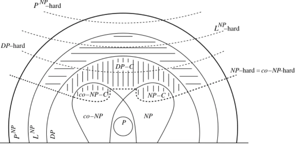
NP-NP −hard L −hard DP NP −hard P L NP P NP co−NP NP NP−C P DP−C
NP−hard = co−NP−hard
co−NP−C
DP
Figure 1: Some classes of complexity.
hard (respectively, co-NP-hard) if there is a Turing reduction from some NP-complete (respectively, co-NP-complete) problem to π [8, p. 113]. Remark 2 Note that with these definitions, NP-hard and NP-hard co-incide [8, p. 114].
The notions of completeness and hardness can of course be extended to classes other than NP or co-NP. NP-hardness is defined differently in [5] and [12]: there, a problem π is NP-hard if there is a polynomial reduction from some NP-complete problem to π; this may lead to confusion (see Section 4).
We also introduce the classes PN P (also known as ∆2in the class hier-archy) and LN P (also denoted by PN P[O(log n)] or Θ2), which contain the decision problems which can be solved by applying, with a number of calls which is polynomial (respectively, logarithmic) with respect to the size of the instance, a subprogram able to solve an appropriate problem in NP (usually, an NP-complete problem); and the class DP [23] (or DIFP [2] or BH2[18], [25], . . .) as the class of languages (or problems) L such that there are two languages L1 ∈ NP and L2∈ co-NP satisfying L = L1∩ L2. This class is not to be confused with NP ∩ co-NP (see the warning in, e.g., [22, p. 412]); actually, DP contains NP ∪ co-NP and is contained in LN P. See Figure 1.
Membership to P, NP, co-NP, DP, LN P or PN P gives an upper bound on the complexity of a problem (this problem is not more difficult than . . .), whereas a hardness result gives a lower bound (this problem is at least as difficult as . . .). Still, such results are conditional in some sense; if
for example P=NP, they would lose their interest. But we do not know whether or where the classes of complexity collapse.
We now consider the satisfiability problems defined in Section 1.1. The problems SAT and 3-SAT are two of the basic and most well-known NP-complete problems [4], [8, p. 39, p. 46 and p. 259]. More generally, k-SAT is NP-complete for k ≥ 3 and polynomial for k = 2. The problem 1-3-SAT, which is obvioulsy in NP, is also NP-complete [24, Lemma 3.5], [8, p. 259], [15, Rem. 3].
In [15] we proved the following.
Proposition 3 [15, Th. 10] For every integer k ≥ 3, the problems U-SAT, U-k-SAT and U-1-3-SAT are equivalent, up to polynomials. ♦ Using results from [2] and [22, p. 415], it is then rather simple to obtain the following result.
Corollary 4 For every integer k ≥ 3,
(a) the decision problems U-SAT, U-k-SAT and U-1-3-SAT are NP-hard (and co-NP-hard by Remark 2);
(b) the decision problems U-SAT, U-k-SAT and U-1-3-SAT belong to
the class DP. ♦
Remark 5 It is not known whether these problems are DP-complete. In [22, p. 415], it is said that “U-SAT is not believed to be DP-complete”.
We are now ready to investigate the problems of Vertex Cover and Domi-nation.
2
Vertex Covers
In this section, we are going to describe three polynomial reductions: U-1-3-SAT →p U-VC and U-1-3-SAT →p U-OVC (Theorem 8),
U-VC →p U-SAT (Theorem 11).
The consequence of these reductions is that U-SAT and U-VC have equiv-alent complexity, that U-VC and U-OVC are NP-hard, and that U-VC belongs to DP. We shall also show that U-OVC belongs to the class LN P.
2.1
Preliminary Results
The following result characterizes the vertices belonging to at least one optimal VC, through the comparison of two vertex cover numbers, and will be used in the (constructive) proof of Proposition 13.
Lemma 6 Let G = (V, E) be a graph. For a given vertex α ∈ V , we consider the following graph: Gα= (Vα, Eα), with
Vα= V ∪ {β1, β2}, Eα= E ∪ {αβ1, αβ2},
where, for 1 ≤ i ≤ 2, βi∈ V . Then α belongs to at least one optimal vertex/ cover in G if and only if φ(G) = φ(Gα).
Proof. (a) Let α be a vertex belonging to at least one optimal vertex cover C in G; then C is a VC in Gα as well, and φ(Gα) ≤ |C| = φ(G).
On the other hand, let C∗ be an optimal VC in Gα. Then obviously α ∈ C∗ and none of the βi’s belongs to C∗. Consequently, C∗ ⊆ V , C∗ is a VC in G, and φ(G) ≤ |C∗| = φ(Gα).
Therefore, with this assumption on α, we have: φ(G) = φ(Gα). (b) Conversely, assume that φ(G) = φ(Gα) for a vertex α ∈ V . Let C∗ be an optimal VC in Gα; again, α ∈ C∗, and none of the βi’s belongs to C∗. Then C∗is a VC in G, it has size φ(Gα) = φ(G), and it contains α. ♦ Proposition 7 [19], [8, p. 46 and p. 190] The decision problem VC is
NP-complete. ♦
Actually, we shall only use the fact that the problem VC belongs to NP, in the proofs of Propositions 13 and 14.
2.2
Uniqueness of Vertex Cover
2.2.1 From U-1-3-SAT to U-VC and U-OVC
Theorem 8 There exists a polynomial reduction from U-1-3-SAT to U-VC and to U-OVC: U-1-3-SAT →p U-VC and U-1-3-SAT →p U-OVC. Proof. Going deeper into the proof of the NP-completeness of the problem Vertex Cover (see [19], [8, pp. 54–56]), which uses a polynomial reduction from 3-SAT and obviously does not convey the uniqueness of the solution, we describe a polynomial reduction from the problem U-1-3-SAT to U-VC and U-OVC, see Figure 2. If the instance of U-1-3-SAT consists of a set C of m clauses over n variables, we construct
– one vertex denoted by X;
– for each clause cj, a triangle Tj= {aj, bj, dj};
– for each variable xi, a component Gi = (Vi = {xi, xi}, Ei = {xixi}) and an auxiliary triangle Ti∗ = {a∗i, b∗i, d∗i} whose vertices are linked to xi, xi and X by the three edges xia∗
i, xid∗i and b∗iX, called “auxiliary membership edges”.
Then we link the components Gi on the one hand, and the triangles Tj on the other hand, according to which literals appear in which clauses
a1 d2 1 b 1 d 1 G x1 b1* d4* a1* x4
G
VC X 1 Tauxiliary membership edges membership edges auxiliary
triangles
Figure 2: Illustration of the graph constructed for the reduction from U-1-3-SAT to U-OVC, with four variables and two clauses, c1= {x1, x2, x3}, c2= {x2, x3, x4}. The sixteen black vertices form the (not unique) optimal vertex cover V∗ corresponding to the (not unique) truth assignment x1= T, x2 = F, x3 = F, x4 = F 1-3-satisfying the clauses. As soon as we set V∗∩ (V1∪ V2∪ V3∪ V4) = {x1, x2, x3, x4}, the other vertices in V∗ are forced.
(“membership edges”): for each clause cj = {ℓ1, ℓ2, ℓ3}, we link ℓ1and aj, ℓ2 and bj, and ℓ3 and dj. We also add the triangular set of edges E′
j = {ℓ1ℓ2, ℓ1ℓ3, ℓ2ℓ3}.
The graph G thus constructed constitutes the instance of U-OVC, and, together with the integer k = 2m + 3n, the instance of U-VC. The order of G is 1 + 3m + 5n.
Note that if V∗is a VC, then each triangle Tj and each auxiliary trian-gle T∗
i contain at least two vertices, each component Giat least one vertex, and |V∗| ≥ 2(m + n) + n = 2m + 3n = k; if |V∗| = k, then V∗ is optimal, and each triangle contains exactly two vertices, each component Giexactly one vertex. We can also observe that, because of the edge sets E′
j, at least two vertices among ℓ1, ℓ2, ℓ3 belong to any VC.
(a) Let us first assume that the answer to U-1-3-SAT is YES: there is a unique truth assignment 1-3-satisfying the clauses of C. Then, by taking, in each Gi, the vertex corresponding to the literal which is TRUE, in every triangle Tj, the two vertices which are linked to the two false literals of cj, and in every auxiliary triangle the vertex linked to X and the one linked to the false literal, we obtain a VC V∗whose size is equal to k = 2m + 3n, which is optimal. Note that X /∈ V∗; in fact, once we have put the n vertices corresponding to the true literals in the VC V∗in construction, we have no choice for the optimal (up to k) completion of V∗: when we take two vertices in Tj, we must take the two vertices which cover the membership edges linked to the two false literals (in Figure 2, the vertices b1, d1 and b2, d2); similarly, we have no choice either for the auxiliary triangles. So, if another
optimal VC V+(of size k) exists, it must have a different distribution of its vertices over the components Gi, still with exactly one vertex in each Gi; this in turn defines a valid truth assignment, by setting xi= T if xi∈ V+, xi= F if xi∈ V+. Now this assignment 1-3-satisfies C, thanks in particular to our observation on the covering of the edges in E′
j. So we have two truth assignments 1-3-satisfying C, contradicting the YES answer to U-1-3-SAT; therefore, V∗ is the only optimal VC (with size k). So we have a YES answer to both U-VC and U-OVC.
(b) Assume next that the answer to U-1-3-SAT is NO: this may be either because no truth assignment 1-3-satisfies the instance, or because at least two assignments do; in the latter case, this would lead, using the same argument as in the previous paragraph, to at least two optimal VC (of size k = 2m + 3n), and a NO answer to both U-VC and U-OVC. So we are left with the case when the set of clauses C cannot be 1-3-satisfied. As seen previously when discussing V+, this implies that no VC of size k exists; this is sufficient to show that the answer is also NO for U-VC.
Assume then that V∗is an optimal VC, of unknown size |V∗| > 2m+3n. Then (i) at least one triangle contains three vertices of V∗, or (ii) at least one component Gi contains two vertices of V∗, or (iii) X ∈ V∗. Assume first that one triangle Tj or one auxiliary triangle T∗
i contains three vertices belonging to V∗; this can happen only if the three membership edges, aux-iliary or not, starting from this triangle are not covered by their other ends (otherwise, we could save one vertex in the triangle). But then, exchanging in V∗one vertex of this triangle with the other end of its membership edge gives another optimal VC, and a NO answer to U-OVC. So we may assume from now on that all the triangles have exactly two vertices in V∗. Assume next that a component Gi has two vertices belonging to V∗; then inside its auxiliary triangle T∗
i, we have at least two possibilities for choosing the two vertices belonging to V∗, and, once again, a NO answer to U-OVC. So we are left with the case when X ∈ V∗, but again, using the same type of argument, there is choice inside the auxiliary triangles. So in all cases, we have a NO answer to U-OVC. ♦ Corollary 9 The decision problems UVC and U-OVC are NP-hard. Proof. Use Theorem 8 and Corollary 4(a). ♦ 2.2.2 An Upper Bound for the Complexity of U-VC
Remark 10 The method carried out in the proof of the following theorem is quite general and can be used with other types of problems, e.g., those involving the existence of a vertex set with bounded size in a graph: roughly speaking, the clauses constructed below in (a) “describe” the problem, those in (b) deal with the size of the set, and finally the clauses in (c) rule out
multiple solutions obtained by permutations, symmetries, . . ., and guarantee the uniqueness. See also the proof of Theorem 24 below.
Theorem 11 There exists a polynomial reduction from U-VC to U-SAT: U-VC →p U-SAT.
Proof. We start from an instance of U-VC, a graph G = (V, E) and an integer k, with V = {x1, . . . , x|V |}; we assume that |V | ≥ 3. We create the set of variables X = {xh
i : 1 ≤ h ≤ |V |, 1 ≤ i ≤ k} and the following clauses:
(a) for each edge xhxℓ∈ E, clauses of size 2k: {xh
1, xh2, . . . , xhk, x ℓ
1, . . . , xℓk}; (b1) for 1 ≤ i ≤ k and 1 ≤ h < ℓ ≤ |V |, clauses of size two: {xh
i, xℓi}; (b2) for 1 ≤ i < j ≤ k and 1 ≤ h ≤ |V |, clauses of size two: {xh
i, xhj}; (c) for 1 ≤ i < k and 1 < ℓ ≤ |V |, for 1 ≤ h < ℓ and i < j ≤ k, clauses of size two: {xℓi, xh
j}.
Note that the number of variables and clauses is polynomial with respect to the order of G, since we may assume that k ≤ |V |.
Assume that we have a unique VC of size k in G, V∗ = {xp1, xp2,
. . . , xpk}, with p1< p2< . . . < pk. Observe that V∗ is optimal (otherwise,
any optimal VC destroys the uniqueness assumption). Define the assign-ment A1 by A1(xpq
q ) = T for 1 ≤ q ≤ k, and all the other variables are set FALSE by A1. This assignment satisfies all the clauses; indeed:
(a) at least one of xh, xℓ belongs to V∗; if, say, xh= xpq ∈ V∗, then by
definition xh
q is set TRUE by A1, and satisfies the clause; (b1) if {xh
i, x ℓ
i} is not satisfied for some h, i, ℓ, then A1(xhi) = A1(xℓi) = T, which would mean that two different vertices are the i-th element in V∗;
(b2) if {xh i, x
h
j} is not satisfied, this means that x
h appears more than once in V∗;
(c) if {xℓ
i, xhj} is not satisfied for some i, ℓ, with h < ℓ and i < j, then A1(xℓ
i) = A1(x h
j) = T. This means that x
ℓ= xpi and xh = xpj; so ℓ = pi,
h = pj. Now h < ℓ implies that pj < pi, but i < j implies that pi < pj, a contradiction.
Is A1 unique? Assume on the contrary that another assignment, A2, also satisfies the constructed instance of U-SAT. By (a), at least one variable xh i or xℓ
j is set TRUE by A2, for every h, ℓ corresponding to an edge xhxℓ, and for some i or j; so if V+is a vertex set which contains the vertex xhas soon as some variable xh
i is set TRUE by A2, then V+is a vertex cover. By (b1), for each i ∈ {1, . . . , k} there is at most one variable with subscript i set TRUE by A2; this tells us that we have constructed a VC with (at most) k elements. Since such a VC is unique by assumption, we can see that A1 and A2have “selected” the same k vertices, i.e., for each pq∈ {p1, . . . , pk},
there is exactly one variable, xpq
q , set TRUE by A1, and, thanks to (b2), exactly one variable, say xpq
s , set TRUE by A2. All the other variables with superscript pq are FALSE by A1 or A2. Then, using (c), we can see that necessarily q = s for every pq, and that A1and A2 must coincide: indeed, assume on the contrary that for some q ∈ {1, . . . , k}, we have q 6= s; we treat the case 1 ≤ q < s ≤ k, the case 1 ≤ s < q ≤ k being similar. Then if we consider the subscripts smaller than s, there must be one, say v, such that there is a superscript pu > pq verifying A2(xpu
v ) = T. Now the clause from (c) {xpu
v , x pq
s } is not satisfied by A2, a contradiction.
So a YES answer for U-VC leads to a YES answer for U-SAT. Assume now that the answer to U-VC is negative. If it is negative because there are at least two VC of size k, then we have at least two assignments satisfying the instance of U-SAT: we have seen above how to construct a suitable assignment from a VC, and different VC obviously lead to different assign-ments. If there is no VC of size k, then there is no assignment satisfying U-SAT, because such an assignment would give a VC of size k, as we have seen above with A2. So in both cases, a NO answer to U-VC implies a NO
answer to U-SAT. ♦
Theorem 12 For every integer k ≥ 3, the problems U-SAT, U-1-3-SAT, U-k-SAT and U-VC have equivalent complexity, up to polynomials.
As a consequence, U-VC belongs to the class DP.
Proof. Simply gather Proposition 3, Theorems 8 and 11, and
Corol-lary 4(b). ♦
Note that it could have been shown directly that U-VC belongs to DP. 2.2.3 Two Upper Bounds for the Complexity of U-OVC
We give a first upper bound on the complexity of U-OVC, because the proof is interesting in itself, because it uses a constructive argument (if there is a unique optimal vertex cover, the algorithm can output it), and because for some problems it is sometimes the only available method and result. In the case of Vertex Cover however, we can improve on Proposition 13, and instead of calling a polynomial number of times an algorithm solving a problem in NP, we need to call it only a logarithmic number of times, see Proposition 14.
Proposition 13 The decision problem U-OVC belongs to the class PN P. In case of a YES answer, one can give the only optimal vertex cover within the same complexity.
Proof. Let A1 be an algorithm solving the problem VC, which is in NP, cf. Proposition 7; using a standard dichotomous process, we obtain an
algorithm A2outputting φ(G) for any graph G, with a logarithmic number of calls to A1.
Let G = (V, E) be any instance of U-OVC, with n vertices. Run A2 for G, then, for each vertex v ∈ V , run A2 for Gv, the graph defined in Lemma 6. By the same lemma, we know, by comparing φ(G) and φ(Gv), whether v belongs to at least one optimal VC in G or not. Let Y = {v1, . . . , vℓ} be the set of vertices with a positive answer; then necessarily ℓ ∈ {φ(G), φ(G) + 1, . . . , n}. Now if ℓ > φ(G), there is more than one optimal VC in G, whereas if ℓ = φ(G), there is only one, namely, Y .
This shows that we can obtain the answer to U-OVC with n + 1 calls to A2, which leads to a polynomial number of calls to an algorithm solving the problem VC, together with negligible operations such as construct-ing Gv. Moreover, we can construct the optimal VC when there is one. ♦ Proposition 14 The decision problem U-OVC belongs to the class LN P. Proof. We use the same algorithm A2 as in the proof of the previous proposition, for any graph G. Then, once we have φ(G), we run an al-gorithm solving U-VC, for the instance consisting of G and φ(G). The answer is YES if and only if there is a unique optimal VC in G. Since the problem VC is in NP and U-VC is in DP (but actually, membership to LN P would suffice), this amounts to a logarithmic number of calls to an algorithm solving a problem in NP, plus one call for a problem in DP. Because DP ⊆LN P, we are done. ♦ Note that using an algorithm for U-VC without knowing φ(G) would lead nowhere, because a NO answer cannot be interpreted: either k < φ(G) and there is no VC, or k ≥ φ(G), but there is more than one VC.
2.3
Related Results: Cliques and Independent Sets
Let G = (V, E) be a graph, and Gc = (V, Ec) be its complement: Ec = {uv : u ∈ V, v ∈ V, u 6= v, uv /∈ E}. Then the following three statements are equivalent: (a) V∗ is a vertex cover in G; (b) V \ V∗ is an independent set in G; (c) V \ V∗ induces a clique in Gc. These relationships are simple enough to make it trivial to polynomially transform the problem VC to any one of the following two problems, and vice-versa:
Instance: A graph G and an integer k. Question: Does G admit
(1) an independent set of size at least k? (2) a clique of size at least k? It follows that
– the problems of a unique clique (with bounded size or optimal) and of a unique independent set (with bounded size or optimal) have the same complexity as U-VC and U-OVC, respectively.
3
Dominating Codes
The approach for dominating codes is quite similar to the one for vertex covers, but slightly more complicated because we shall have to study suc-cessively 1-domination, then r-domination for general r.
After some necessary preliminary results, we are going to prove, for r ≥ 1, the polynomial reductions
U-3-SAT →p U-DC1and U-3-SAT →p U-ODC1(Theorem 18), U-DC1 →p U-DCr and U-ODC1 →p U-ODCr(Theorem 20),
U-DCr→p U-DC1and U-ODCr →p U-ODC1 (Proposition 22), U-DC1 →p U-SAT (Theorem 24).
The consequence of these reductions is that U-DCr and U-ODCr are NP-hard. Also, U-SAT and U-DCr have equivalent complexity; as a result, U-DCr belongs to DP. We shall also show that U-ODCr belongs to the class LN P.
3.1
Preliminary Results
The following lemma will be used in the proof of Theorem 20. Lemma 15 Let r ≥ 1 be any integer and let G∗
uv = (Vuv∗, Euv∗ ) be the graph defined as follows:
Vuv∗ = {u, v} ∪ {αi: 1 ≤ i ≤ r − 1} ∪ {βi,j: 1 ≤ i ≤ r − 1, 1 ≤ j ≤ 3r}, Euv∗ = {uα1, α1α2, . . . , αr−1v} ∪
∪ {αiβi,1, βi,1βi,2, . . . , βi,rβi,r+1, . . . , βi,2r−1βi,2r : 1 ≤ i ≤ r − 1} ∪ ∪ {βi,rβi,2r+1, βi,2r+1βi,2r+2, . . . , βi,3r−1βi,3r : 1 ≤ i ≤ r − 1}, see Figure 4 further down. Then γr(G∗
uv) = r, C1 = {u} ∪ {βi,r : 1 ≤ i ≤ r − 1} and C2= {v} ∪ {βi,r : 1 ≤ i ≤ r − 1} are two optimal r-dominating codes in G∗
uv, and any optimal r-dominating codes in G∗uv contains W = {βi,r : 1 ≤ i ≤ r − 1}.
Proof. Because the r − 1 vertices βi,2r must be r-dominated by some codeword, at least r − 1 codewords are necessary. But no vertex can simul-taneously r-dominate βi,2r and u or v, so at least one more codeword is required, and γr(G∗
uv) ≥ r. On the other hand, it is quite straightforward to check that C1 and C2 are r-dominating codes, of size r, so that they
are optimal, and γr(G∗uv) = r. Finally, for a given i ∈ {1, . . . , r − 1}, only βi,rcan r-dominate both βi,2r and βi,3r, and so βi,rbelongs to any optimal
r-dominating code. ♦
Also note that, for any given i with 1 ≤ i ≤ r−1, the vertex βi,rr-dominates exactly αi and βi,j, for 1 ≤ j ≤ 3r.
The following lemma, which characterizes the vertices belonging to at least one optimal dominating code, through the comparison of two r-domination numbers, is very similar to Lemma 6 for vertex covers; it will be used for Proposition 26. It is a simplified version of [14, Cor. 2]. Lemma 16 Let G = (V, E) be a graph, and let r ≥ 1 be any integer. For a given vertex α ∈ V , we consider the following graph: Gα= (Vα, Eα), with
Vα= V ∪ {βi: 1 ≤ i ≤ r}, Eα= E ∪ {αβ1} ∪ {βiβi+1: 1 ≤ i ≤ r − 1}, where for i ∈ {1, . . . , r}, βi ∈ V . Then α belongs to at least one optimal/ r-dominating code in G if and only if γr(G) = γr(Gα). ♦ Proposition 17 [8, p. 75 and p. 190, for r = 1], [14, Prop. 9] Let r ≥ 1 be any integer. The decision problem DCris NP-complete. ♦ Actually, we shall only use the fact that DCr belongs to NP, for Proposi-tions 26 and 27. Note that the proofs of Proposition 17 do not deal with the problem of the uniqueness of a solution.
3.2
Uniqueness of Dominating Code
3.2.1 From U-3-SAT to U-DC1 and U-ODC1
Theorem 18 There exists a polynomial reduction from U-3-SAT to U-DC1 and to U-ODC1: U-3-SAT →p U-DC1 and U-3-SAT →p U-ODC1. Proof. The construction of a graph is common to the two reductions, then we add an integer k for U-DC1. We start from an instance of U-3-SAT, a collection C of m clauses over a set X of n variables. For each variable xi ∈ X , 1 ≤ i ≤ n, we construct the graph Gi = (Vi, Ei) as follows (see Figure 3):
Vi= {xi, xi, ai, bi} ∪ {αi,ℓ: 1 ≤ ℓ ≤ 3}, Ei = {xiai, xiai, aibi} ∪ {xiαi,ℓ, xiαi,ℓ: 1 ≤ ℓ ≤ 3}.
Then for each clause cj, 1 ≤ j ≤ m, containing three literals, we create one vertex, Aj, and link it to the three vertices corresponding, in the graphs Gi, to the literals of cj. This is our graph G; its order is 7n + m. Additionally, we set k = 2n for U-DC1.
a
iA
jx
ix
ib
i i,1α
Figure 3: The graph G constructed in the proof of Theorem 18.
Note already that, because of the vertices bi and αi,ℓ, any optimal 1-dominating code in G contains xi or xi, and ai or bi, for all i ∈ {1, . . . , n}. Consequently, γ1(G) ≥ 2n = k.
We claim that there is a unique solution to 3-SAT if and only if there is a unique optimal 1-dominating code, and if and only if there is a unique 1-dominating code of size (at most) k, in G.
(1) Assume first that there is a unique truth assignment satisfying all the clauses. We construct the following code C: for i ∈ {1, . . . , n}, among the vertices xi ∈ Vi, xi ∈ Vi, we put in C the vertex xi if the literal xi has been set TRUE, the vertex xiif the literal xi is FALSE, and we add ai. Then C is a 1-dominating code; in particular, every vertex Aj is 1-dominated by at least one codeword since every clause contains at least one true literal. The code C has size k = 2n and is optimal. Moreover, once xi or xi is a codeword, the only way to complete the code with not more than n additional codewords is to take ai, so that xi or xi is 1-dominated by C, since no Aj is a codeword. The code C is unique: suppose on the contrary that C∗ is another 1-dominating code of size 2n in G. Then |C∗ ∩ Vi| = 2 for all i ∈ {1, . . . , n}, no Aj is a codeword, and exactly one of xi and xi is in C∗. This defines a valid truth assignment for X , by setting xi = T if xi ∈ C∗, xi = F if xi ∈ C∗. Since C 6= C∗, this assignment is different from the assignment used to build C. But the fact that C∗ 1-dominates Aj for all j shows that there is a codeword xi or xi 1-dominating Aj, which means that the clause cj is satisfied. Therefore, we have a second assignment satisfying the instance of 3-SAT, a contradiction. We can conclude that both problems, U-DC1 and U-ODC1, also have a YES answer.
(2) Assume next that the answer to U-3-SAT is NO: this may be either because no truth assignment satisfies the instance, or because at least two assignments do; in the latter case, this would lead, using the same argument as previously, to at least two optimal 1-dominating codes of size k = 2n, and a NO answer to U-DC1 and to U-ODC1. So we are left with the case when the set of clauses C cannot be satisfied. This implies that no 1-dominating code of size k = 2n exists, as seen with C∗; this is sufficient
to end the proof for U-DC1, but we have to go on for U-ODC1: assume then that C is an optimal 1-dominating code of unknown size |C| > 2n. We know that each Vi contains at least two codewords. Where can the extra codeword(s) be?
Suppose that a vertex Aj0is a codeword. If the three vertices in {xi, xi:
1 ≤ i ≤ n} to which Aj0 is linked are codewords, then Aj0 could have been
saved. So there is at least one neighbour of Aj0, say xi0, which does not
belong to C. Now xi0 ∈ C, xi0 is 1-dominated by Aj0 ∈ C, and either
C ∩ Vi0 = {xi0, ai0} or C ∩ Vi0 = {xi0, bi0} may be part of an optimal
solution, i.e., we have a NO answer for U-ODC1.
So we can assume from now on that no Ajis a codeword, and that there is at least one set Vi0containing at least three codewords. If it is more than
three, then codewords can be spared. If it is exactly three, then xi0and xi0
are codewords, so that some vertices Aj linked to them are 1-dominated by C thanks to xi0 and xi0: otherwise, two codewords inside Vi0 would
have been sufficient. Now we have a choice for the third codeword in Vi0:
it can be either ai0 or bi0.
In all cases, we have proved that there can be several optimal 1-domina-ting codes, i.e., we have a NO answer for G, the constructed instance of
U-ODC1. ♦
Remark 19 The fact that all the clauses have degree three has no im-portance whatsoever, and the proof could also work using any problem U-k-SAT, k ≥ 3, or U-SAT. Only the degrees of the vertices Aj would be affected.
3.2.2 Extension to r ≥ 2
Theorem 20 Let r ≥ 2 be any integer. There is a polynomial reduction from U-ODC1 to U-ODCr and from U-DC1 to U-DCr: U-ODC1 →p U-ODCr and U-DC1 →p U-DCr.
Proof. This proof is inspired by the proof of Proposition 9 in [14]. We start from a graph G = (V, E) and an integer k for U-DC1, and the same graph G for U-ODC1.
The graph G∗= (V∗, E∗) is common to the reduction to U-DCrand to U-ODCr(see Figure 4), and is defined by setting, for each edge e = uv ∈ E,
Ve∗ = {αe,i : 1 ≤ i ≤ r − 1} ∪ {βe,i,j : 1 ≤ i ≤ r − 1, 1 ≤ j ≤ 3r}, E∗
e = {uαe,1, αe,1αe,2, . . . , αe,r−2αe,r−1, αe,r−1v} ∪
{αe,iβe,i,1, βe,i,1βe,i,2, . . . , βe,i,rβe,i,r+1, . . . , βe,i,2r−1βe,i,2r : 1 ≤ i ≤ r − 1} ∪ {βe,i,rβe,i,2r+1, βe,i,2r+1βe,i,2r+2, . . . , βe,i,3r−1βe,i,3r: 1 ≤ i ≤ r − 1}.
vertices r v u vertices r r − 1 vertices
Figure 4: How the edge e = uv ∈ E gives V∗
e and Ee∗. The black vertices on the branches are the vertices βe,i,r.
Then we set
V∗= V ∪ (∪e∈EVe∗), E∗= ∪e∈EEe.∗
Finally, for U-DCr, we put k∗= k + (r − 1)|E|. The order of G∗ is |E|(r − 1)(3r + 1).
(1) We claim that an instance of U-ODC1 is positive if and only if the corresponding instance of U-ODCr is.
(a) First, we assume that there is a YES answer in G for U-ODC1: there is a unique optimal 1-dominating code C in G. Let W be the set consisting of the (r − 1)|E| vertices βe,i,r, e ∈ E, 1 ≤ i ≤ r − 1. Note that W r-dominates exactly V∗\ V , and that, by Lemma 15, any optimal r-dominating code in G∗ contains W . Because C is 1-dominating in G, clearly C∗ = C ∪ W is r-dominating in G∗. Note in particular that two vertices u and v at distance 1 in G are at distance r in G∗.
Because moreover C is optimal, the code C∗ is also optimal: assume on the contrary that C+ is an optimal r-dominating code in G∗, with |C+| < |C∗|. We proceed as in the proof of Proposition 9 in [14]: the subcode C+\ W must r-dominate all the vertices in V , and if a codeword in V∗\ V performs part of this task, it can be replaced by a vertex in V . After such replacements have possibly been made, we have a code C×such that C×∩ V r-dominates, in G∗, all the vertices in V ; this implies that in G, C×∩ V 1-dominates all the vertices. But |C×∩ V | ≤ |C+\ W | < |C∗\ W | = |C| = γ1(G), i.e., |C×∩ V | < γ1(G), which is impossible.
Finally, because we assumed that C was the only optimal 1-dominating code in G, the code C∗ = C ∪ W is the only optimal r-dominating code in G∗. Suppose on the contrary that C+ is another optimal code in G∗: |C+| = |C∗| = |C| + |W |.
(i) C+∩ V = C+\ W , or, equivalently, (V∗\ V ) ∩ C+= W . Then, as we have already seen, C+∩V is 1-dominating in G, and either C+∩V = C∗∩V , which leads to C+ = C∗, or C+∩ V 6= C∗∩ V , in which case we have two
optimal 1-dominating codes in G, C+\ W and C∗\ W = C. In both cases, we have a contradiction.
(ii) C+∩ V 6= C+\ W . Then there is at least one codeword z ∈ C+ belonging to some V∗
e \ {βe,i,r: 1 ≤ i ≤ r − 1}, with e = uv ∈ E. Then z must r-dominate u or v or both; otherwise, z is useless and can be saved. For the same reason, u /∈ C+ and v /∈ C+; but then (C+\ {z}) ∪ {u} and (C+ \ {z}) ∪ {v} are also both r-dominating in G∗. By similarly replacing all the t codewords in (V∗\ W ) \ V , t ≥ 1, by codewords in V , we have 2t codes included in V ∪ W which are all r-dominating in G∗, which implies that their intersections with V all are 1-dominating in G; moreover, these intersections have size (at most) |C+| − |W | = |C|, i.e., are optimal. Finally, there are at least two of them, so at least one is different from C, contradicting its uniqueness.
This shows that a YES answer to U-ODC1 leads to a YES answer to U-ODCr.
(b) And a NO answer to U-ODC1 leads to a NO answer to U-ODCr, since two optimal 1-dominating codes in G, C1 and C2, give two optimal r-dominating codes in G∗, C1∪ W and C2∪ W .
This ends the part for U-ODCr.
(2) We claim that an instance of U-DC1 is positive if and only if the corresponding instance of U-DCris.
(a) First, we assume that there is a YES answer for U-DC1: there is a unique 1-dominating code C with size at most k in G. Obviously, C is optimal, otherwise any optimal 1-dominating code in G would contradict the uniqueness of C. Consider the code C∗ = C ∪ W in G∗, of size k + (r − 1)|E| = k∗. Exactly as in Step (1) of this proof, C∗ is r-dominating, is optimal, and is the only r-dominating code of size at most k∗ in G∗. So the answer to U-DCr is also positive.
(b) Next, we assume that the answer to U-DC1 is NO: either there is no 1-dominating code with size at most k in G, or there is more than one. In the latter case, we have more than one r-dominating code with size at most k∗in G∗: simply add the set W to the codes in G. So we assume that we are in the first case. This implies in particular that γ1(G) > k; using the same argument as in Step (1), we can see that γr(G∗) > k +(r −1)|E| = k∗, and there is no r-dominating code with size at most k∗ in G∗. In all cases, the answer to U-DCr is NO. ♦ Corollary 21 Let r ≥ 1 be any integer. The decision problems U-DCr and U-ODCr are NP-hard. ♦ Proposition 22 Let r ≥ 2 be any integer. There is a polynomial reduction from U-DCrto U-DC1 and from U-ODCr to U-ODC1: U-DCr →p U-DC1 and U-ODCr →p U-ODC1.
Proof. Let (G, k) be an instance of U-DCr and G be an instance of U-ODCr, for r ≥ 2. The instance for U-DC1 is simply (Gr, k), and Gr for U-ODC1, where Gris the r-th power of G: obviously, by Lemma 1, there is a unique 1-dominating code of size k in Grif and only if there is a unique r-dominating code of size k in G, and there is a unique optimal 1-r-dominating code in Grif and only if there is a unique optimal r-dominating code in G. ♦ Corollary 23 Let r1≥ 1 and r2≥ 1 be any integers.
(a) The decision problems U-DCr1 and U-DCr2 are equivalent, up to
polynomials.
(b) The decision problems U-ODCr1 and U-ODCr2 are equivalent, up
to polynomials. ♦
3.2.3 An Upper Bound for the Complexity of U-DCr
Theorem 24 There exists a polynomial reduction from U-DC1to U-SAT: U-DC1 →p U-SAT.
Proof. We fully use Remark 10: we start from an instance of U-DC1, a graph G = (V, E) and an integer k, with V = {x1, . . . , x|V |}; we assume that |V | ≥ 3. We create the set of variables X = {xh
i : 1 ≤ h ≤ |V |, 1 ≤ i ≤ k} and the following clauses:
(a) for each vertex xh ∈ V with neighbours xh1, . . . , xhs, clauses of
size (s + 1)k: {xh 1, xh2, . . . , xhk, x h1 1 , . . . , x h1 k , . . . , x hs 1 , . . . , x hs k }; (b1) for 1 ≤ i ≤ k and 1 ≤ h < ℓ ≤ |V |, clauses of size two: {xh
i, xℓi}; (b2) for 1 ≤ i < j ≤ k and 1 ≤ h ≤ |V |, clauses of size two: {xh
i, xhj}; (c) for 1 ≤ i < k and 1 < ℓ ≤ |V |, for 1 ≤ h < ℓ and i < j ≤ k, clauses of size two: {xℓ
i, xhj}.
Compared to the proof of Theorem 11, only the clauses in (a) are different: they convey the fact that among the vertices xh, xh1, . . . , xhs, at least one
must be put in a 1-dominating code. The proof then goes exactly as for
Theorem 11. ♦
By Proposition 22 or its corollary, this immediately implies that there is a polynomial reduction from U-DCrto U-SAT.
Theorem 25 Let r ≥ 1 and k ≥ 3 be any integers. The problem U-DCr has complexity equivalent to that of U-SAT, U-k-SAT and U-1-3-SAT.
As a consequence, U-DCr belongs to the class DP. ♦ Note that it could have been shown directly that U-DCrbelongs to DP.
3.2.4 Two Upper Bounds for the Complexity of U-ODCr The (constructive) membership of U-ODCrto the class PN P and the mem-bership to LN P can be proved in exactly the same way as in Section 2.2.3 for U-OVC. This time, it is the characterizing Lemma 16 which must be used, together with Proposition 17.
Proposition 26 For r ≥ 1, the decision problem U-ODCr belongs to the class PN P. In case of a YES answer, one can give the only optimal r-dominating code within the same complexity. ♦ Proposition 27 For r ≥ 1, the decision problem U-ODCrbelongs to LN P. ♦
4
Conclusion
Corollary 4 states that the three problems, U-SAT, U-1-3-SAT and U-k-SAT (k ≥ 3), are equivalent and lie somewhere in the vertically hatched area of Figure 5, but probably not in DP-C, cf. Remark 5.
Theorems 12 and 25 state that U-VC and U-DCr, r ≥ 1, have the same complexity as the above three problems, and consequently are located in the same hatched area.
We have also established that the decision problems OVC and U-ODCr, r ≥ 1, belong to the class LN P, see Propositions 14 and 27, and that they are NP-hard, see Corollaries 9 and 21. This means that they lie within the areas that are hatched horizontally or vertically. Moreover, all the problems U-ODCr are equivalent between each other, by Corollary 23(b).
We have the same conclusions for Cliques and Independent Sets (see Section 2.3).
In [2], the authors wonder whether
(A) U-SAT is NP-hard, but here we believe that what they mean is: does there exist a polynomial reduction from an NP-complete problem to U-SAT ? i.e., they use the second definition of NP-hardness;
finally, they show that (A) is true if and only if (B) U-SAT is DP-complete.
So, if one is careless and considers that U-SAT is NP-hard without checking according to which definition, one might easily jump too hastily to the conclusion that U-SAT is DP-complete, which, to our knowledge, is not known to be true or not. As for U-3-SAT, we do not know where to locate it more precisely either; in [3] the problems U-k-SAT and more particularly U-3-SAT are studied, but it appears that they are versions where the given set of clauses has zero or one solution, which makes quite a difference with our problem.
NP −hard L −hard DP NP −hard P L NP P NP co−NP NP DP−C P
NP−hard = co−NP−hard
NP−C co−NP−C
DP
Figure 5: Some classes of complexity: Figure 1 re-visited.
Open problem 1 (general). For k ≥ 3 and r ≥ 1, improve the location of U-SAT, U-k-SAT, U-1-3-SAT, U-VC, U-OVC, U-DCrand U-ODCr, within the classes of complexity.
Open problem 2. It is easy to establish that U-OVC →p U-ODC1 (and U-OVC →pU-ODCr, r ≥ 2). What more can be said about the relationship between U-OVC and U-ODC1 (and U-ODCr)?
Open problem 3 (conjecture). Under the assumption P6=NP, U-OVC is not equivalent to U-VC, and U-ODCris not equivalent to U-DCr, r ≥ 1. Finally, in [6] (respectively, [9]), characterizations of the trees (respectively, the block graphs, which are a class of graphs including the trees) admitting a unique optimal 1-dominating code are given. This result, together with a linear algorithm determining optimal 1-dominating codes in block graphs, then allows to show that the sub-problem of U-ODC1 where the instance is any block graph is linear.
Open problem 4. Is it possible to extend this kind of result to any integer r ≥ 1? to other classes of graphs?
References
[1] J.-P. BARTH´ELEMY, G. D. COHEN and A. C. LOBSTEIN: Algo-rithmic Complexity and Communication Problems, London: Univer-sity College of London, 1996.
[2] A. BLASS and Y. GUREVICH: On the unique satisfiability problem, Information and Control, Vol. 55, pp. 80-88, 1982.
[3] C. CALABRO, R. IMPAGLIAZZO, V. KABANETS and R. PATURI: The complexity of Unique k-SAT: an isolation lemma for k-CNFs, Journal of Computer and System Sciences, Vol. 74, pp. 386–393, 2008. [4] S. A. COOK: The complexity of theorem-proving procedures, Pro-ceedings of 3rd Annual ACM Symposium on Theory of Computing, pp. 151–158, 1971.
[5] T. CORMEN: Algorithmic complexity, in: K. H. Rosen (ed.) Hand-book of Discrete and Combinatorial Mathematics, pp. 1077–1085, Boca Raton: CRC Press, 2000.
[6] M. FISCHERMANN: Block graphs with unique minimum dominating sets, Discrete Mathematics, Vol. 240, pp. 247–251, 2001.
[7] M. FRANCES and A. LITMAN: On covering problems of codes, The-ory of Computing Systems, Vol. 30, No. 2, pp. 113–119, 1997.
[8] M. R. GAREY and D. S. JOHNSON: Computers and Intractability, a Guide to the Theory of NP-Completeness, New York: Freeman, 1979. [9] G. GUNTHER, B. HARTNELL, L. R. MARKUS and D. RALL: Graphs with unique minimum dominating sets, Congressus Numer-antium, Vol. 101, pp. 55–63, 1994.
[10] T. W. HAYNES, S. T. HEDETNIEMI and P. J. SLATER: Fundamen-tals of Domination in Graphs, New York: Marcel Dekker, 1998. [11] E. HEMASPAANDRA, H. SPAKOWSKI and J. VOGEL: The
com-plexity of Kemeny elections, Theoretical Computer Science, Vol. 349, pp. 382–391, 2005.
[12] L. HEMASPAANDRA: Complexity classes, in: K. H. Rosen (ed.) Handbook of Discrete and Combinatorial Mathematics, pp. 1085–1090, Boca Raton: CRC Press, 2000.
[13] I. S. HONKALA and A. C. LOBSTEIN: On the complexity of calcu-lating the minimum norm of a binary code, Proc. Workshop on Coding and Cryptography ’99, pp. 21–27, Paris, 1999.
[14] O. HUDRY and A. LOBSTEIN: More results on the complexity of domination problems in graphs, International Journal of Information and Coding Theory, to appear.
[15] O. HUDRY and A. LOBSTEIN: Some complexity considerations on the uniqueness of solutions for satisfiability and colouring problems, submitted.
[16] O. HUDRY and A. LOBSTEIN: On the complexity of determining whether there is a unique Hamiltonian cycle in a graph, submitted. [17] O. HUDRY and A. LOBSTEIN: Unique (optimal) solutions:
complex-ity results for identifying and locating-dominating codes, submitted. [18] D. S. JOHNSON: A catalog of complexity classes, in: Handbook of
Theoretical Computer Science, Vol. A: Algorithms and Complexity, van Leeuwen, Ed., Chapter 2, Elsevier, 1990.
[19] R. M. KARP: Reducibility among combinatorial problems, in: R. E. Miller and J. W. Thatcher (eds.) Complexity of Computer Computa-tions, pp. 85–103, New York: Plenum Press, 1972.
[20] A. McLOUGHLIN: The complexity of computing the covering radius of a code, IEEE Trans. Inform. Th., Vol. 30, pp. 800–804, 1984. [21] A. MERTZ: On the complexity of multicovering radii, IEEE Trans.
Inform. Th., Vol. 50, pp. 1804–1808, 2004.
[22] C. H. PAPADIMITRIOU: Computational Complexity, Reading: Addison-Wesley, 1994.
[23] C. H. PAPADIMITRIOU and M. YANNAKAKIS: The complexity of facets (and some facets of complexity), Journal of Computer and System Sciences, Vol. 28, pp. 244–259, 1984.
[24] T. J. SCHAEFER: The complexity of satisfiability problems, Proceed-ings of 10th Annual ACM Symposium on Theory of Computing, pp. 216–226, 1978.