Mécanismes contrôlant les anomalies de température de surface de la mer et de précipitation au cours de deux années contrastées 2010 et 2012 dans l'Atlantique tropical

THÈSE

THÈSE

En vue de l’obtention du

DOCTORAT DE L’UNIVERSITÉ DE

TOULOUSE

Délivré par : l’Université Toulouse 3 Paul Sabatier (UT3 Paul Sabatier)

Présentée et soutenue le 06 Mars 2019 par :

Antonio VASCONCELOS NOGUEIRA NETO

Mécanismes contrôlant les anomalies de température de

surface de la mer et de précipitation au cours de deux

années contrastées 2010 et 2012 dans l’Atlantique tropical

JURY

Jean-Pierre CHABOUREAU

LA Président du Jury

Pierre CAMBERLIN CRC Rapporteur

Christophe MAES LOPS Rapporteur

Pierrick PENVEN LOPS Examinateur

Julien JOUANNO LEGOS Examinateur

Gaelle De COETLOGON

LATMOS Examinatrice

École doctorale et spécialité :

SDU2E : Océan, Atmosphère, Climat Unité de Recherche :

Météo-France

Centre National de Recherches Météorologiques (CNRM, UMR 3589) Directeur(s) de Thèse :

Hervé GIORDANI et Philippe PEYRILLE Rapporteurs :

Peu d’études ont été consacrées à la documentation des processus pilotant l’évolu-tion de l’ITCZ maritime sur l’Atlantique (AMI). La présente étude fournit une analyse de l’évolution de l’océan et de l’atmosphère de l’Atlantique tropicale pour deux années contrastées en Température de Surface de la Mer (TSM), 2010 et 2012, qui ont été respec-tivement les années les plus chaudes et les plus froides observées au cours de la période 1982-2015.

Les mécanismes à l’origine des anomalies interannuelles et saisonnières de la TSM sont d’abord explorés via un bilan thermique dans la couche de mélange océanique (CMO) ef-fectué à partir de flotteurs Argo, de données satellitaires et des réanalyses atmosphériques ERA-Interim pour la période 2007-2012. Le flux de chaleur latente en surface s’est avéré être sous-estimé de 20 W.m−2 conduisant à un mélange vertical erroné dans l’ensemble du domaine. La correction de ce flux de surface a permis d’assimiler le résidu à un mélange vertical turbulent à la base de la couche de mélange d’intensité réaliste. Une fois corrigé, le bilan de la CMO montre que les anomalies de TSM observées en 2010 et 2012 ont été générées par une anomalie de vent liée à une anomalie de flux de chaleur latente sur l’Atlantique nord en hiver. L’advection horizontale induite par le vent joue cependant un rôle fondamental pour équilibrer les flux de surface dans l’Atlantique Sud en 2012. Ces résultats montrent que l’Atlantique tropical nord est une région clé pour la génération des anomalies de TSM observées en 2010 et 2012.

La deuxième partie de l’étude étudie la mise en place des anomalies pluviométriques de 2010 et 2012 et les mécanismes associés. En moyenne saisonnière, les précipitations de 2010 ont été plus intenses sur une grande partie du bassin tandis que celles de 2012 présentaient un dipôle méridien avec un maximum de précipitations décalé de 5◦ au nord par rapport à la climatologie. Un bilan d’eau intégré verticalement a montré que l’advec-tion d’humidité est la principale contribul’advec-tion à l’anomalie de précipital’advec-tion pour les deux années, notamment via l’anomalie de vent horizontal.

À l’échelle intrasaisonnière, une analyse des régimes de pluie révèle que les pluies fortes étaient plus fréquentes en 2010 alors que en 2012 les pluies faibles étaient plus fréquentes. La relation entre les précipitations et certains facteurs clés tels que la TSM et l’eau précipitable dans la zone de l’AMI montrent qu’en 2010, le seuil de TSM pour le déclenchement des pluies est supérieur à celui de 2012. La relation eau précipitable -pluie montre également l’existence d’un seuil d’eau précipitable pour le déclenchement des pluies différent selon les années et selon la température de la troposphère. On montre ainsi que les conditions atmosphériques plus chaudes de 2010 ont contribué à «atténuer» l’effet de l’anomalie de TSM via le mécanisme de Clausius-Clapeyron. La pluie est également modulée par le tourbillon vertical qui est plus faible en 2010 qu’en 2012 à régimes de pluie équivalents, ce que souligne le rôle des perturbations atmosphériques. Une analyse spectrale des précipitations montre que les ondes d’Est Africaines, dans la gamme 2 - 10 jours, expliquent l’essentiel des différences observées dans la variabilité des pluies entre 2010 et 2012.

Enfin, un ensemble de simulations réalisées avec le modèle atmosphérique à aire limitée Méso-NH a été utilisé pour comprendre les contributions de l’océan et de l’atmosphère aux anomalies de pluies de 2010 et 2012. Les pluies simulées en changeant la TSM de 2010 par celle de 2012 et en gardant les conditions latérales de 2010 sont très proches de

Abstract

The Atlantic Marine ITCZ (AMI) is a regional manifestation of the ITCZ over the warm water of the tropical Atlantic oceans. Few studies have been devoted to document the processes driving the evolution of the SST and precipitation, most of which were centered on the eastern side of the basin.

The present study provides an analysis of the evolution of the ocean and the at-mosphere over the Western part of the Atlantic for two contrasted years in Sea Surface Temperature (SST), 2010 and 2012, that were respectively the warmest and coldest years observed during the 1982-2015 period.

The causes of interannual and seasonal anomalies of SST are first explored via an ocea-nic mixed-layer (ML) heat budget performed from Argo floats, satellite-based data and ERAI-Interim atmospheric reanalysis for the period 2007-2012. The surface latent heat flux was found to be under-estimated by 20 W/m2 and conducted to erroneous vertical mixing in the whole domain. Correction of these surface fluxes yielded to residuals which were assimilated to vertical turbulent mixing at the mixed-layer base, which fell into rea-listic range. Once corrected, the ML budget shows that the observed SST anomalies in 2010 and 2012 were generated by anomalous wind stress and, consequently, anomalous latent heat flux in the north Atlantic during winter. The wind-induced horizontal advec-tion plays a fundamental role in balancing the surface flux in the south Atlantic in 2012. The north tropical Atlantic appears as a key region for the generation of the SSTs pattern observed in 2010 and 2012.

The second part of the study analyses the building of the 2010 and 2012 rainfall anomalies and the underlying mechanisms. On seasonal average, 2010 shows a more intense rainfall over the basin while 2012 exhibits a meridional dipole of precipitation with a rainfall maximum shifted 5 degrees north of its climatological location. An analysis of the water budget integrated vertically indicates that the anomalous vertical advection of moisture is the leading term that contributed to the precipitation anomalies for both years and that anomalous horizontal wind has the greatest contribution to this term.

At the intraseasonal scale, an analysis of the precipitation regimes reveal that 2010 favoured more frequent heavy rainfall than 2012 while 2012 was characterised by more frequent lighter rain. The relationships between the precipitation and some key factors such as SST and precipitable water (PW) are analysed within the AMI to understand how deep convection was altered under different SST conditions. The main results is that the 2010 shows a higher SST threshold than 2012 for strong rainfall to occur. The precipitation - PW relationships shows the existence of a threshold of precipitable water too, which depends on the years and the tropospheric temperature. It is underlined that the atmospheric warmer conditions in 2010 vs 2012 acted to "damp" the SST anomaly via Clausius-Clapeyron mechanism, i.e. by increasing the water vapour saturation threshold of the atmosphere. A spectral analysis of precipitation revealed that African Easterly Waves at periods of 2-10 days explain most of the difference in the variability of precipitation between both years.

Finally a set of simulation realised with the limited-area atmospheric model Meso-Nh was used to understand the contribution of the ocean and the atmosphere to the anomalous precipitation for 2010. Sensitivity experiments to the SST and initial/lateral boundary conditions were performed. The rainfall simulated by Meso-NH when forcing the model with the SST from 2012 and keeping the lateral boundary conditions to those of 2010 are very close to the rainfall obtained for 2010. It shows that the key factor to determine the 2010 rainfall anomaly is not the SST but the atmospheric properties provided by the lateral boundary conditions i.e. the anomalous horizontal wind and the tropospheric temperature.

Summary

Résumé . . . . i

Abstract . . . . iii

List of tables . . . . vi

List of figures . . . vii

0.1 Introduction (Français) . . . xii

. . . xii

I Introduction . . . . 1

1.1 The tropics and the general circulation . . . . 2

1.1.1 Defining the tropical region . . . 2

1.1.2 The tropical troposphere and the large scale circulation . . . 3

1.1.3 Upper ocean circulation . . . 7

1.1.4 The Intertropical Convergence Zone (ITCZ) . . . 10

1.1.5 Mechanisms of ocean-atmosphere interactions . . . 11

1.2 The tropical Atlantic and Atlantic Marine ITCZ (AMI) . . . 14

1.2.1 First view of the AMI . . . 14

1.2.2 Multi-scale variability of the AMI - Rainfall and SST . . . 16

1.2.3 Ocean mixed layer processes . . . 16

1.2.4 Convection over the tropical oceans . . . 24

1.3 Main objectives . . . 29

II Main Data Set . . . 31

2.1 Argo profiles . . . 32

2.2 OSCAR and GEKCO currents. . . 32

2.3 OISST . . . 33

2.4 Precipitation TRMM . . . 33

2.5 ERA-Interim reanalyses . . . 33

2.6 OAflux evaporation . . . 34

2.7 Meso-NH numemircal model . . . 34

III Heat budget in the oceanic mixed layer . . . 36

3.1 Mixed layer heat storage in the Tropical Atlantic from Argo observations 37 3.1.1 Summary of the article . . . 37

3.2 Article : Seasonal and interannual mixed layer heat budget in the western tropical Atlantic using Argo float (2007-2012) . . . 40

Abstract . . . 41

1. Introduction . . . 41

2. Materials and Methods . . . 43

IV Tropical Atlantic in contrasted years : comparisons between 2010 and

2012 . . . 66

4.1 Overview . . . 67

4.2 The AMI during 2010 and 2012 . . . 67

4.2.1 Large scale context . . . 67

4.2.2 Seasonal mean anomalies . . . 71

4.2.3 Dynamical patterns . . . 74

4.3 Water budget . . . 77

4.3.1 Spatial distribution of the anomalies . . . 77

4.3.2 Perturbed convergence term . . . 86

4.4 Distributions of the precipitation . . . 90

4.4.1 Rainfall regimes . . . 90

4.4.2 Factors controlling the precipitation . . . 93

4.4.3 Intraseasonal variability . . . 104

4.5 Conclusions . . . 110

V Meso-NH model . . . 112

5.1 Overview . . . 113

5.2 Model simulations . . . 113

5.3 Impact of SST resolution on precipitation . . . 114

5.4 Differences between 2010 and 2012 . . . 116

5.5 Effect of the MesoNH convection scheme . . . 118

5.6 Meridional distribution of Pr and water budget (20120-2012). . . . 120

5.7 Conclusions . . . 123

VI Conclusions and perspectives . . . 125

6.1 Conclusion . . . 125

6.2 Perspectives. . . 128

VII Conclusions et perspectives (Français) . . . 130

7.1 Conclusion . . . 130

7.2 Perspectives. . . 133

Liste des tableaux

3.1 Data Set of Satellite-Derived Products Used to Estimate the Mixed-Layer Heat Budget . . . . 43 3.2 Main Characteristics of the Seasonal Cycles of the SSTr, SSTargo, and T

Series in Each Box With Minimum, Maximum Values and Months, and Range of the Seasonal Cycle (◦C) . . . . 50 3.3 Mean Values of the Different Terms of the Budget Each Box (W m−2) . . . 51 3.4 Main Increment δx i Used to Estimate Errors in Each Heat Budget

Com-ponents . . . 51 3.5 Mean Errors on the Different Terms of the Budget Each Box (W m22)(W m−2) 52

4.1 Total and relative difference (mm) between 2010 and 2012 considering all regimes (total) ans for each regimes (R1, R2 and R3) . . . 93 5.1 Simulations performed with the Meso-NH model for the tropical

Atlan-tic. Shows the atmospheric boundary conditions, SST forcing, convective scheme and the nomenclature used. . . 114

List of figures

0.1 Série temporelle d’anomalies mensuelles de TSM Reynolds (◦C) dans

l’At-lantique Tropical [20◦S − 20◦S]. Les deux lignes horizontales tiretées

repré-sentent + − 2 écarts-types. . . xv 0.2 Série temporelle d’anomalies mensuelles de précipitation TRMM (mm.day−1)

dans l’Atlantique Tropical [20◦S − 20◦S]. . . xvi

1.1 Vertical structure of the zonal-averaged temperature (left) and specific hu-midity (right) during from June to August (top panels) and from December to February (bottom panel). Adpted from Beucher (2010) . . . 4 1.2 Schematic view of the Hadley circulation. Abbreviations : TTL – Tropical

tropopause layer, ITCZ – Intertropical convergence zone. . . 5 1.3 Schematic view of the east–west atmospheric circulation along the

longi-tude–height plane over the Equator. The cell over the Pacific Ocean is referred to as the Walker Circulation. From (Lau et Yang, 2015) . . . 7 1.4 Schematic view of the wind-driven currents which form the subtropical

gyres of each oceanic basin. . . 8 1.5 (left) Annual, boreal summer (JAS), and boreal winter (JFM) mean

pre-cipitation (mm.day−1). Orography is shown by black contours at 1-km intervals. (right) Zonal-mean precipitation. Data are taken from TRMM for 1998–2014. From Adam et al. (2016a) . . . 11 1.6 Annual-mean climatology of SST(◦C, colors), rain rate Pr (mm.day−1,contours)

greater than 5 mm.day−1 and surface winds (m.s−1) in the tropical Atlan-tic. SST and wind data are from ERA-Interim and Pr from TRMM. . . 15 1.7 [1998-2014] climatology of SST (colors), contours of rain rate (Pr) greater

than 5 mm.day−1 and winds (m.s−1) in the tropical Atlantic during March-April and July-August. SST and wind data are from ERA-Interim and Pr from TRMM. . . 16 1.8 SST and atmospheric circulation anomaly composites during the peak

phase of the Atlantic Niño. (a) SST anomalies (K) ; (b) 200 mb poten-tial velocity anomalies (106_m2_.s−1_{) and divergent wind anomalies (m.s}−1_{) ;}

(c) 500 mb vertical velocity anomalies (10−4mb.s−1, contours) ; (d) Atlan-tic Walker circulation anomalies indicated by the [2.5◦S and 2.5◦N ] mean

divergent wind and vertical velocity ; and (e) Atlantic Hadley circulation anomalies depicted as the [40◦W and 0◦] divergent wind and vertical velo-city anomalies. Positive values are shaded. From Wang (2004) . . . 19 1.9 SST and atmospheric circulation anomalies for positive-negative phase of

the meridional gradient mode. (a) SST anomalies (K) ; (b) 200 mb velo-city potential (106_m2_.s−1_{) and divergent wind anomalies (m.s}−1_{) ; (c) 500}

mb vertical velocity anomalies (10−4mb.s−1) ; and (d) Hadley circulation anomalies indicated by the mean [50◦W and 10◦W ] divergent wind and

vertical velocity anomalies. Positive phase period of 1966 − 70 and the ne-gative phase period of 1971 − 75. Positive values are shaded. From Wang (2004) . . . 21 1.10 SST–convection relation in monthly (a) and daily (b) data of the 1◦lat–long

bins of area 160◦E − 130◦W , 5◦S − 25◦N . (c) and (d) give the same for

130◦W − 100◦W , 5◦S − 25◦N . Vertical bars and number of observations are

as in Figure 2 (the linear correlation coefficient and number of observational pairs are marked at top left). From Sabin et al. (2013) . . . 25

1.11 (a) Pickup of ensemble average precipitation hPi, conditionally averaged by 0.3-mm bins of column water vapor w for 1-K bins of the vertically averaged tropospheric temperature ¯T , for the eastern Pacific. Lines show

power-law fits above the critical point of the form (2). (b) As in (a), but for 2 mm bins of the lower troposphere integrated saturation value ¯qsatLT

for the eastern Pacific. Inset : As in (a), but for 5 mm bins of the vertically

integrated saturation value ¯qsat. From Neelin et al. (2009) . . . 27

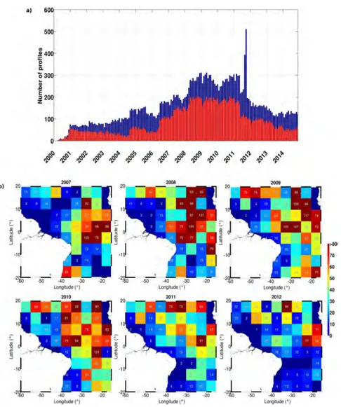
3.1 (a) Number of Argo float profiles from 2000 to 2014 (blue bars) and number of remained profiles after our quality control (red bars). (b) Number of Argo float profiles within 58 3 58 boxes for the years 2007–2012. . . . 44

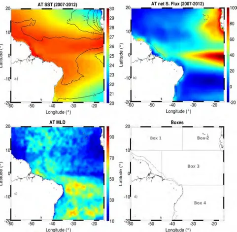
3.2 Comparison between mean (a) OSCAR and (b) GEKCO currents (arrows) during the 2007–2012 period. Current magnitude shaded (m s21). (c) Diffe-rence of magnitude of the currents OSCAR-GECKO during the same period. 45 3.3 General mean field of the main parameters considered to describe the regio-nal heterogeneities of the WTA. (a) SST (contours indicate the standard deviation), (b) net surface heat flux, (c) MLD obtained from Argo floats, and (d) the four regions chosen to describe the SST variability and the mixed-layer heat budget. Northern tropical Atlantic (boxes 1 and 2), wes-tern equatorial Atlantic (box 3), and south tropical Atlantic (box 4). . . . . 48

3.4 Seasonal cycles of T (red curve), SSTrargo (blue curve), and SSTr (black curve) during the period 2007–2012 for the five zones (temperature scale on the left in 8C). Standard errors are indicated by shaded colors. The number of profiles per box is also indicated with blue bars. . . . 49

3.5 Relative contributions (in W m22) of the various terms on the right-hand side of equation (1) obtained with advection and entrainment computed from OSCAR and GEKCO currents. Corrected S.Flux and RES are shown. . . . 53

3.6 Mean vertical turbulent mixing (blue) and standard deviation (red) obtained from Argo profiles in the WTA during 2007–2012. The star indicates the magnitude of the residual term at the mean observed MLD. . . . 54

3.7 Heat budget terms of equation (1) in box 1 (heat storage in black, surface fluxes in blue, horizontal advection in red, entrainment in green, and ho-rizontal advection and entrainment with OSCAR product in full line and dash with GEKCO). Top right figure shows the monthly mean shortwave radiation (red) and latent heat flux (blue) ; the middle right figure is the me-ridional (triangle) and zonal (square) components of the wind stress and in the bottom right figure the zonal (square) and meridional advection (triangle). 54 3.8 Same as Figure 3.7, but for box 2. . . . 55

3.9 Same as Figure 3.7, but for box 3. . . . 55

3.10 Same as Figure 3.7, but for box 4. . . . 56

3.11 Mean seasonal cycle of the residual term in each box. . . . 57

3.12 Monthly mean SST anomalies with respect to 1982–2012 reference period. The series of WTA averaged SSTs has been deseasonalized and detrended over the reference period. Read and blue shaded bars highlight the 2010 and 2012 years, respectively. Dotted lines represents 62r (standard deviation) of the series. . . . 57

3.13 Monthly zonal averaged SSTr (solid lines) and T (dots) between 2010 (red), 2012 (blue), and the mean for the 2007–2012 period (black). Data were averaged every 18 of latitude. . . . 58

3.15 Wind stress anomalies from ERA-Interim colocated to Argo float profiles for each year from 2007 to 2012 in (a) box 1, (b) box 2, and (c) box 5. . . . 60 3.16 Accumulated heat budget for the period October–March (a–d) 2009/2010

and (e–h) 2011/2012. Local heat storage (black), surface flux (blue), and sum of oceanic terms (red). Dotted lines represent the mean for the 2007–2012 period. . . . 61 4.1 Annual mean of SST (◦C) and Precipitation rate Pr (mm.day−1) and

res-pective anomalies in 2010 (a,c) and 2012 (b,d). The boxes in (a,b) indicate the AMI region considered between 2 − 10◦N in both years . . . . 68 4.2 First (a) and second (b) leading EOF modes of SST over the [1998-2014]

period. Corresponding standardized time series are shown in the bottom panel. The numbers on top of each panel show the percentage of variance explained by each EOF. The EOFs are performed on the year-average SST anomaly relative to the mean annual cycle. In (c,d) standardization is made using the interannual variance of each EOF time series. In (a,b) the EOF contours are every 0.1◦C . . . . 69 4.3 Monthly time series of SST (◦C ; a) and rain rate (mm.dat−1; b) during

MJJA 2010 (yellow), 2012 (blue) and climatology (black) averaged in the AMI box. . . 70 4.4 Anomalies of SST (◦C ; a-b), rain rate (Pr ; mm.day−1; c-d) and PW (mm ;

e-f) during MJJA 2010 and 2012 in the tropical Atlantic. . . 73 4.5 Anomalies of column-integrated temperature (Ta ; K) during MJJA 2010

(top) and 2012 (botton) in the tropical Atlantic. . . 74 4.6 Vertical structure of vertical velocity ( P a.s−1; colours) meridional wind

(m.s−1, contours) averaged between 20 − 30◦W in 2010 (a) and 2012 (b).

Black dashed and continuous lines represents negative and positive values, respectively. In (a,b) dashed green lines mark the position of the maximum of vertical velocity and position of the AMI of each year. . . 75 4.7 (a,b) Wind vectors and zonal wind anomalie (m.s−1 at 600 hP a for 2010

and 2012. (c,d) same as (a,b) except for zonal wind shear between 600 and 1000 hPa (m.s−1). . . 76 4.8 Spatial distribution of the moisture storage anomalies (∆[∂P W_∂t ] ; colors)

related to 1982-2014 period averaged over MJJA 2010 (a) and 2012 (b). Contour lines represent the ∆[P r] from TRMM. Continues and dotted lines represent positive and negative anomalies, respectively. The term is expressed in (mm.day−1). . . 78 4.9 spatial distribution of the total advection anomalies (∆[Adv] ; colors)

rela-ted to 1982-2014 period averaged over MJJA 2010 and 2012. Contour lines represent the ∆[P r] from TRMM. Continues and dotted lines represent positive and negative anomalies, respectively. The terms are expressed in (mm.day−1) . . . 79 4.10 Spatial distribution of Hadv and Vadv anomalies (colors) related to

1982-2014 period averaged over MJJA 2010 and 2012. Contour lines represent the ∆[P r] from TRMM. Continues and dotted lines represents positive and negative anomalies, respectively. The terms are expressed in (mm.day−1). . 80 4.11 Spatial distribution of evaporation anomalies (∆[E] ; colors) related to

1982-2014 period averaged over MJJA 2010 (a) and 2012 (b). Contour lines represent the ∆[P r] from TRMM. Continues and dotted lines repre-sents positive and negative anomalies, respectively. The term is expressed in (mm..day−1) . . . 81

4.12 Meridional profile of ∆[Adv] (orange), ∆[E] − [P ] (green) and residual (black) anomalies average between 20◦W − 30◦W in MJJA 2010 (a) and

2012 (b). The terms are expressed in (mm.day−1) . . . 82 4.13 Meridional profile of horizontal advection (∆[Hadv], blue), vertical

advec-tion (∆[V adv], red), evaporaadvec-tion (∆[E], gray) and precipitaadvec-tion (-∆[P r] ; pink) anomalies average between 20◦W −30◦W in MJJA 2010 (a) and 2012

(b). The terms are expressed in (mm.day−1). . . 83 4.14 Meridional profile of mean and [E] and ∆[E] from ERA-I (black) and

OAflux (green), average between 20◦W − 30◦W in MJJA 2010 and 2012.

The terms are expressed in (mm.day−1) . . . 84 4.15 the same as in figure 4.14, but for the precipitation rate Pr (mm.day−1)

from ERA-I and TRMM. . . 85 4.16 Spatial distribution of the column-integrated −div∆[ ~U q] and −div∆[ ~U ][¯q]

in 2010 (a, c) and 2012 (b, d). The terms are expressed in (mm.day−1). . . 87 4.17 Spatial distribution of the difference between 2010 and 2012 of the −div∆[ ~U q]

(a) and −div∆[ ~U ][¯q] (b) terms (mm.day−1). . . 88 4.18 Meridional section of each term of the the Eq 7 averaged between 20◦W and

30◦W in 2010 (right) and 2012 (left).The terms are expressed in mm.day−1. 89 4.19 Meridional section of the horizontal component of the decomposed

trans-port of humidity averaged between 20◦W and 30◦W in 2010 (right) and

2012 (left). The terms are expressed in mm.day−1. . . 90 4.20 PDF of daily precipitation rate (mm.day−1) in the AMI box during MJJA.

The climatology (1998-2014) is represented by the black line, the 2010 and 2012 years are represented by the yellow and blue lines, respectively. The gray lines are the PDFs for each year of the reference period. . . 91 4.21 Comparisons of the box-averaged number of days of precipitation rate in

each regime identified and for each month, during MJJA. . . 92 4.22 Box-averaged accumulated time series of daily Pr during MJJA. a) The

total precipitation range (all regimes). b-d) The same as (a), but for each regime identified. . . 94 4.23 Conditionally-average rain rate (Pr ; mm.day−1) by bins of SST (◦C) in the

AMI box during MJJA. The climatology, 2010 and 2012 are represented by black, yellow and blue lines, respectively. Gray lines represent the Pr-SST relationship for each year of the reference period (1998-2014). Bins of SST were defined by quantiles of 5%. . . 96 4.24 Conditionally-average rain rate (Pr ; mm.day−1) by bins of PW (mm) in

AMI box during MJJA. The climatology, 2010 and 2012 are represented by black, yellow and blue lines, respectively. Gray lines represent the Pr-PW relationship for each year of the reference period (1998-2014). Bins of PW were defined by quantiles of 2%. . . 97 4.25 Conditionaly average rain rate (Pr ; mm.day−1) by bins of the RP W in the

AMI box during MJJA. The climatology, 2010 and 2012 are represented by black, yellow and blue lines, respectively. Gray lines represent the Pr-RP W

relationship for each year of the reference period (1998-2014). Bins of RP W

4.27 Conditionaly-average rain rate (Pr ; mm.day−1) by bins of vertical velocity (ω ; P a.s−1) in AMI box during MJJA at 850 hP a (a) and 200 hP a (b). The climatology, 2010 and 2012 are represented by black, yellow and blue lines, respectively. Gray lines represent the Pr-ω relationship for each year of the reference period (1998-2014). Bins of ω were defined by quantiles of 2%. . . 102 4.28 Conditionaly-average rain rate (Pr ;mm.day−1) by bins of (a) zonal wind

shear (1000-600 hP a, m.s−1) and (b) vorticity (ζ) in the AMI box during MJJA. The climatology, 2010 and 2012 are represented by black, yellow and blue lines, respectively. Gray lines represent the Pr-shear and Pr-ζ relationship for each year of the reference period (1998-2014). Bins of wind shear and ζ were defined by quantiles of 2%. . . 103 4.29 Standard deviation difference between 2010-2012 of the total Pr std (mm2_;

a) and the 2-90 days filtered Pr (b) during MJJA. . . 105 4.30 Spectral analysis of Pr in 2010 and 2012. (a) spectrum normalized by the

variance and (b) the normalized spectrum multiplied by the frequency to highlight low frequencies. . . 106 4.31 AMI box-averaged time series of the deviation of Pr (mm.day−1) from

the mean MJJA ( ¯P r) and the spectral bands identified from the spectral

analysis. The dashed line indicate the standard deviation of total anomaly of Pr in each year. . . 108 4.32 Relative variance of Pr filtered at 2-10 days with respect to the total

va-riance during MJJA in 2010 (a) and 2012 (b) in the Tropical Atlantic. . . . 109 4.33 The composite of Pr (mm.day−1; colors) and zonal wind at 925 hPa based

on the box 31 − 36◦W and 2 − 7◦N . . . 110

5.1 Differences between simulations LBC10-sst-N10 and LBC10-sst-E10 for SST (◦ C ; a) and Pr (mm.day−1; b) in June 2010. These differences illus-trate the effect of high resolution SST on the precipitation pattern from the model. . . 115 5.2 Differences between simulations LBC10-sst-N10 and LBC12-sst-N12 for

SST (◦ C ; a) Pr (mm.day−1; c) in June 2010 and 2012. The difference between years is also shown for ERA-I SST (b) and TRMM Pr (b). It illus-trate the capability of the model to reproduce the differences of SST and Pr observed from reanalysis and observations (ERA-I and TRMM) between 2010 end 2012. . . 117 5.3 Differences between simulations LBC10-sst-N10 and LBC10-sst-N12 for

SST (◦ C ; a) Pr (mm.day−1; b) in June 2010. This comparison allow to evaluate the effect of the SST in 2012 on the atmospheric conditions of 2010.118 5.4 Comparison between Pr (mm.day−1) from simulations with different

convec-tion scheme of the Meso-NH model for June 2010. . . 119 5.5 Comparison between the Pr (mm.day−1) from the simulation

Expl.-LBC10-sst-N10 and TRMM in June 2010. . . 119 5.6 Meridional profile of precipitation Pr (mm.day−1) from each simulation

compared to precipitation from TRMM (mm.day−1) in June 2010 and 2012.121 5.7 Meridional profile of the difference of each term of the water budged (in

0.1

Introduction (Français)

L’océan et l’atmosphère sont les composantes les plus importantes du système Terre et jouent un rôle prépondérant sur le climat global. Le rayonnement solaire est le moteur principal des mouvements dans l’océan et l’atmosphère. Ils sont responsables de la redistribution de l’excédent d’énergie absorbée dans les tropiques vers les pôles.

L’énergie absorbée par l’océan dans la région équatoriale est reémise vers l’atmo-sphère sous la forme de flux de chaleur turbulent (sensible ou latent). Ces flux réchauffent la colonne atmosphérique par le bas, destabilisent l’atmosphère et génèrent un mouvement ascendant associé à de la divergence en haute troposphère. Cette circulation marque la branche ascendante de la circulation méridienne appelée circulation de Hadley qui corres-pond à la Zone de Convergence Intertropicale (ZCIT). Son principal rôle dans le système climatique est la redistribution méridienne de l’énergie accumulée à l’équateur.

La ZCIT est une des plus remarquables caractéristiques des régions tropicales. Elle est définie comme une bande zonale de fortes précipitations qui encercle tout le globe le long de l’équateur en moyenne annuelle. La présence de la ZCIT est associée à une zone de vents faibles et une forte convergence des alizés. La convection profonde associée à la ZCIT libère d’importantes quantités d’énergie dans l’atmosphère par libération de chaleur latente, qui est le principal moteur de la circulation globale (Back et Bretherton, 2009; Xie, 2009; Beucher, 2010).

La ZCIT est associée à une zone où les températures de surface de la mer (TSM) sont supérieures à 27◦C tout au long de l’année. Cette zone gouverne le déplacement

méridien saisonnier de la ZCIT, qui atteint les latitudes les plus basses entre janvier et avril, avant de migrer vers le nord jusqu’à 8◦N - 9◦N en août.

Les théories actuelles considèrent la ZCIT en moyenne globale et proposent des théories pour expliquer sa position, son déplacement ainsi que l’intensité des pluies asso-ciées. Elles mettent en avant le rôle du flux net d’énergie dans l’atmosphère, à savoir le bilan d’énergie entre le sommet de l’atmosphère et la surface terrestre (Schneider et al., 2014; Adam et al., 2016b), et soulignent le rôle des flux de chaleur latente et sensible à la surface. Il n’existe en revanche aucun cadre théorique pour expliquer les variations

régio-le Pacifique.

La ZCIT apparaît comme un phénomène couplé entre océan et atmosphère (Beu-cher, 2010). Dans les bassins Pacifique et Atlantique, la formation d’une langue d’eau froide (LEF) sous l’effet des vents de surface (Philander et al., 1984) impacte le dépla-cement de la ZCIT et le déclenchement des moussons africaine (Caniaux et al., 2011) et sud-américaine. Plus généralement la convection atmosphérique est alimentée par le contenu thermique océanique via les flux de surface. Une régulation s’établit lorsque le ré-servoir d’énergie est épuisé la convection meurt. Cette vision schématique est un exemple emblématique du couplage océan-atmosphère.

A grande échelle la TSM interagit avec la circulation de basses couches à travers les gradients de pression (Lindzen et Nigam, 1987; Small et al., 2008). Tomas et Webs-ter (1997) montrent une dynamique différente de la ZCIT selon l’intensité du gradient de pression de surface atravers l’Equator, qui est intimement relié à la TSM. Back et Bretherton (2009) ont en effet montré que la convergence de la surface et le mouvement vertical au-dessous de 850 hPa étaient fortement lié au gradient de pression en surface associé au gradient de température et donc directement lié au gradient de TSM. Les mo-difications de la circulation de la Couche Limite Atmosphérique (CLA) induites par la TSM affectent les régimes de précipitations en modulant la flottabilité dans la CLA et l’entraînement à son sommet. De fait les zones les plus documentées sur océan sont les zones de LEF, là où les gradients de TSM sont suffisamment forts pour agir comme un forçage de la circulation atmosphérique de basses couche (Small et al., 2008; de Coetlogon et al., 2014; Diakhaté et al., 2016) sur les océans Pacifique et Atlantique.

A l’échelle de la convection plusieurs études montrent que le déclenchement de la convection profonde est associé à un seuil de TSM (Graham et Barnett, 1987; Johnson et Xie, 2010; Sabin et al., 2013). On observe un seuil de TSM autour de 27.5◦C au-delà les

précipitations augmentent exponentiellement avec la TSM. Par contre au-delà de 29◦C les

pluies diminuent. Ce type de relation est facilement observée sur les régions avec un fort gradient de TSM, comme à l’est de l’Atlantique et du Pacifique équatorial (Sabin et al., 2013). En revanche il n’y a pas de seuil universel de TSM et on observe une dépendance géographique de ce seuil.

Neelin et al. (2009) proposent une théorie alternative au rôle direct de la SST et observent une variation exponentielle des précipitations avec l’eau précipitable qui est

plus indépendante de la région considérée que la TSM. Les deux approches ne sont pas for-cément contradictoires mais soulignent que le lien entre l’océan et les précipitations n’est pas direct, passant à la fois par les flux de surface, des effets thermiques et dynamiques sans doute régionaux qui au final rendent nécessaire l’étude de chaque bassin.

Dans ce cadre général, l’Atlantique tropical est également le lieu d’interactions entre océan et atmosphère à différentes échelles dont le bord est, avec la présence d’une LEF, a été relativement plus documenté que la région ouest. La LEF Atlantique a été décrite en termes de processus océaniques et atmosphériques (Caniaux et al., 2010; Wade et al., 2011; Giordani et al., 2013) comme résulat d’un forçage par les vent de surface mais aussi préconditionné par l’upwelling équatorial (Giordani et Caniaux, 2011).

À l’échelle interannuelle, deux principaux modes de variabilité affectent l’océan (TSM, contenu en chaleur) et l’atmosphère (position et intensité de la ZCIT) (Xie et Car-ton, 2004; Wang, 2004; Ruiz-Barradas et al., 2000). L’un est le mode équatorial, semblable au El Niño dans le Pacifique bien qu’indépendant et de plus faible amplitude que celui-ci, il se traduit par un réchauffement de l’Atlantique tropical et notamment par une varia-tion d’intensité de la LEF. L’autre mode de variabilité est un mode méridien traduisant un gradient marqué de TSM entre l’Atlantique tropical nord et sud. Au-delà de facteurs régionaux, la variabilité du climat de l’Atlantique tropical répond également à l’influence du phénomène El Niño Souther Oscillation (ENSO). Cette influence est observée quelques mois après le pic de la phase ENSO et affecte la position saisonnière moyenne de la ZCIT et l’intensification des périodes humides et de sécheresse sur l’Amérique du Sud tropicale.

Dans l’Atlantique tropical le déplacement méridien de la ZCIT représente la principale caractéristique de la variabilité saisonnière dans l’Atlantique tropical (Hasten-rath, 1984; Folland et al., 1986; Nobre et Shukla, 1996). Sur l’Atlantique tropical plusieurs études montrent que la ZCIT affecte le climat subcontinental, comme par exemple, le nord et le nord-est du Brésil, l’Afrique de l’Ouest et la mer des Caraïbes (Hastenrath, 1984; Nobre et Shukla, 1996; Folland et al., 1986; Parker, 1988; Parker et Folland, 1988).

Du côté océanique, la variabilité de la TSM est généralement analysée en considé-rant les processus en jeux dans la Couche de Mélange Océanique (CMO). De nombreuses étude ont été réalisées à partir d’observations (Foltz et al., 2003; Wade et al., 2011; Foltz

TSM dans différentes régions de l’Atlantique tropical. Yu et al. (2006) ont en particulier divisé l’Atlantique tropical en deux zones : la première, au nord de 10◦N et au sud de

5◦S, où les changements de TSM sont pilotés par les flux de surface et une deuxième

ré-gion dans la bande 10◦S − 5◦N , où les processus dynamiques océaniques dominent. C’est

dans la partie Est de cette région équatoriale que la plupart des études sur la CMO et le couplage océan-atmosphère se sont concentrés. Par contre sur la partie ouest du bassin, aussi bien la CMO et les causes de la variablité de la TSM (Cintra et al., 2015; Servain et Lazar, 2010) que la dynamique de la ZCIT sur l’océan ont été peu documentés.

L’objectif principal de cette thèse est de documenter l’ouest du bassin Atlantique Tropical en terme de variabilité de la TSM et des pluies. Pour cela deux années très contrastées en TSM ont été choisies, 2010 et 2012, qui ont été présentées dans les rapports climatiques et océanographiques comme deux années exceptionelles (Sodré, 2013; Marengo et al., 2013).

Figure 0.1: Série temporelle d’anomalies mensuelles de TSM Reynolds (◦C) dans l’At-lantique Tropical [20◦S − 20◦S]. Les deux lignes horizontales tiretées représentent + − 2

écarts-types.

La Figure 0.1 montre que l’anomalie de TSM en 2010 et 2012 atteint respective-ment +1.1◦C et −0.7◦C, ce qui représente des anomalies supérieures à deux écarts types

et confirme le caractère exceptionnel de ces deux années. Ces anomalies ont coïncidé avec un extrême de pluies au nord-est du Brésil et une forte activité cyclonique en 2010, et une sécheresse marquée au Brésil en 2012 avec l’apparition d’algues Sargasses à partir de 2011 (Sodré, 2013; Marengo et al., 2013; Marengo et Bernasconi, 2015; Lim et al., 2016;

Wang et Hu, 2016).

Les années 2010 et 2012 sont également contrastée en précipitation. La Figure 0.2 montre qu’en 2010 on observe des fortes anomalies positives de précipitation (> 1

mm.day−1) pendant l’été dans l’Atlantique tropical. En 2012 ces anomalies sont negatifs et relativement plus faibles (< 1mm.day−1).

Figure 0.2: Série temporelle d’anomalies mensuelles de précipitation TRMM (mm.day−1) dans l’Atlantique Tropical [20◦_{S − 20}◦_S].

Ces deux années exceptionnelles proposent un bon cadre de travail pour étudier les mécanismes de variabilité de la TSM et ses impacts sur la dynamique atmosphérique en se focalisant sur l’ouest de bassin tropical.

Dans un premier temps la partie océanique est traitée en présentant un bilan de chaleur dans la CMO à partir des flotteurs ARGO. L’objectif de cette partie est d’iden-tifier et quand’iden-tifier les processus dans la CMO et à l’interface air-mer responsables de la variabilité interannuelle et saisonnière de la TSM. Cette étude a fait l’objet d’un article publié dans le journal scientifique "Journal Geophysical Research". Dans cette étude on a pu documenter l’origine des anomalies de TSM sur l’Atlantique tropical en 2010 et 2012.

La deuxième partie de la thèse (chapitres 4 et 5) se concentre sur la description et l’analyse de la ZCIT et des précipitations en 2010 et 2012. A partir des réanalyses du Centre Européen à Moyen Terme (ERA Interim ,Dee et al. (2011)), une analyse des

Une analyse des années 2010 et 2012 à l’échelle intrasaisonnière est réalisée sous l’angle des relations TSM - pluie et eau précipitable - pluie, permettant une extension des travaux existant dans la littérature à d’autres régions et d’autres paramètres. Les contrastes entre ces deux années en termes de régimes de pluies et les échelles des varia-bilité intrasaisonnières sont également documentés.

La dernière partie de cette thèse exploite un jeu de simulations Méso-NH pour mettre en avant le rôle de la TSM dans la construction de l’anomalie de pluies et confirme les résultats obtenus précédement avec les réanalyses.

Les conclusions et les perpectives pour la suite de cette thèse cloturent le ma-nuscrit.

CHAPTER I

Introduction

1.1 The tropics and the general circulation . . . . 2

1.1.1 Defining the tropical region . . . 2

1.1.2 The tropical troposphere and the large scale circulation . . . 3

1.1.2.1 Meridional circulation - The Hadley cell . . . 4

1.1.2.2 Zonal circulation - The Walker cell . . . 6

1.1.3 Upper ocean circulation . . . 7

1.1.3.1 Wind-driven Surface currents . . . 7

1.1.3.2 Atlantic current system . . . 8

1.1.4 The Intertropical Convergence Zone (ITCZ) . . . 10

1.1.5 Mechanisms of ocean-atmosphere interactions . . . 11

1.2 The tropical Atlantic and Atlantic Marine ITCZ (AMI) . . . 14

1.2.1 First view of the AMI . . . 14

1.2.2 Multi-scale variability of the AMI - Rainfall and SST . . . 16

1.2.3 Ocean mixed layer processes . . . 16

1.2.3.1 Interannual modes of variability of the tropical Atlantic and AMI . 18 1.2.3.2 ENSO teleconnections . . . 21

1.2.3.3 Intraseasonal variability of convection . . . 22

1.2.4 Convection over the tropical oceans . . . 24

1.2.4.1 Link SST-convection . . . 24

1.2.4.2 Link precipitable water-convection . . . 26

1.2.4.3 link dynamic factors-convection . . . 28

1.1

The tropics and the general circulation

1.1.1 Defining the tropical region

Geographically the tropics are defined as the regions between the tropic of Cancer and the tropic of Capricorn. They mark the latitudinal band where the solar declination angle can reach 90◦ and the mean annual temperature is not less than 18◦C. In

oceano-graphy and meteorology the boundaries of the tropical region are usually related to the position of the high pressure zones. These zones are related to anticyclonic motion obser-ved over oceans in the north and south hemisphere. From this definition, the boundaries of tropical region can vary significantly at seasonal and interannual time scales following the variability of ocean and atmospheric circulation.

In terms of solar radiation this region is where the annual radiation budget is positive. So, the tropical region is characterized by an excess of energy, while at the poles the net radiation is negative due to a deficit of incoming energy. This imbalance of energy drives most of the ocean and atmospheric motion which are the main components of the Earth climate system.

The ocean and atmospheric circulations are responsible for the redistribution of the surplus of energy from the tropical regions to the poles. From the atmospheric point of view the tropics are characterized by the presence of the low surface pressure close to the Equator (pressure trough), persistent northeasterly and southearterly trade winds and net upward motion, which is associated with the surplus of heating in this region. These characteristics define the circulation pattern related to the Intertropical Convergence Zone (ITCZ). The latter is an important feature of tropical regions and represents the ascending branch of the main meridional atmospheric circulation known as the Hadley circulation.

From the oceanic point of view, the tropics are marked by a strong meridional SST gradient with annual mean maximum in a zonal band just north of the equator which is correlated to the mean position of the ITCZ. In terms of oceanic circulation this region presents a complex system of currents which encompass wind-driven surface currents, counter-currents and subsurface currents. They are fundamental to the transport of heat and mass between the hemispheres as part of the Meridional Overturning circulation (MOC).

The tropical region is the place of important components of the physical cycles of the Earth system. These cycles are maintained by the constant exchange of matter, energy and momentum between ocean and atmosphere which modulate the global climate.

1.1.2 The tropical troposphere and the large scale circulation

The troposphere is the lowest layer of the atmosphere which interacts with the surface and where the atmospheric circulation plays its role in controlling the weather and climate. In the tropics the troposphere has specific characteristics that differ from other regions. The vertical structure of the zonally-averaged temperature (Figure 1.1) shows that the meridional gradient in the tropical troposphere is weak. Because of that the troposphere in the tropics is "quasi-barotropic" (Beucher, 2010).

The temperature is maximal at lower levels and gradually decreases upward to the top of the troposphere (tropopause). That is because the troposphere is heated from the surface by turbulent heat flux (latent and sensible heat) and long waves. The latent heat released in higher levels by deep tropical convective clouds also contributes to warm the troposphere in this region (Schneider et Lindzen, 1977; Lindzen et Hou, 1988). As a result, the tropical troposphere expands and the tropopause height is about 7 km higher than at the poles.

Due to the excess of heating, the tropical troposphere has greater capacity to "hold" water vapour. Consequently the vertical distribution of the specific humidity in the troposphere is very correlated to that of temperature. Then, large amount of water vapour are observed close to the surface with significant decrease with height (Figure 1.1). The amount of water vapour in the tropical region is determinant for convection in the ITCZ. The low-troposphere maximum of temperature and specific humidity present seasonal changes which are associated with the seasonal displacement of the ITCZ.

Figure 1.1: Vertical structure of the zonal-averaged temperature (left) and specific hu-midity (right) during from June to August (top panels) and from December to February (bottom panel). Adpted from Beucher (2010)

.

In the tropical troposphere the large scale circulation is intimately linked to the intensity and position of the ITCZ. In the next sections we describe the main meridional and zonal circulation in the tropical region to contextualize the ITCZ into the atmospheric general dynamics .

1.1.2.1 Meridional circulation - The Hadley cell

The mean meridional atmospheric circulation is known as the Hadley cell. This name was done in honour of George Hadley who was one of the first to propose a convec-tion cells in the atmosphere that would transport heat from the Equator to the poles. Today, this circulation is recognized as the main atmospheric large scale mechanism of redistribution of the excess of heat from the Equator to subtropical regions. It is funda-mental to maintain the energetic equilibrium of the climate system.

Large-scale motion of air in the troposphere are related to the horizontal pressure gradient generated by the meridional differences on surface heating. Thus, the air flows from high to low pressure and is subject to the effect of Earth rotation which reduces the meridional component as it approaches the Equator. The ascending branch is located over the low pressure regions which marks the meteorological Equator (or ITCZ). It is

surrounded by two descending branches over the subtropical high pressure regions in each hemisphere (anticyclones).

Around low pressure regions, the warm and moist winds converge near the surface leading to an upward vertical motion which is associated with the increase of cloud cover. In the upper troposphere the winds diverge toward the poles and descend in high pressure regions which are associated with clean sky, despite the occurrence of low level clouds. In the Atlantic ocean the anticyclones of Azores and St. Helen mark the descending branches of the Hadley cell around 30◦ of latitude in both the north and south hemisphere. The divergence of near surface winds at each anticyclone are at the origin of the northeast and southeast trade winds. As these winds approach to the equatorial regions they warm and are charged by humidity which will feed the ITCZ and close the meridional overturning Hadley circulation.

The Hadley circulation is largely modulated by the seasonal cycle, thus it follows the meridional migration of the equatorial low pressure region which are related to the warmer SSTs and the ITCZ. During July-August the northward shift of the Hadley cell is related to a weak northeasterly trade and the intensification of southeasterly trade in the central and western part of the basin, which are generated by the St Helena high, located over the southeast Atlantic. March-April marks the period of the northeast trade wind intensification which is related to the southernmost position of the ITCZ and the weakening of southeast winds.

Figure 1.2: Schematic view of the Hadley circulation. Abbreviations : TTL – Tropical tropopause layer, ITCZ – Intertropical convergence zone.

1.1.2.2 Zonal circulation - The Walker cell

The Walker circulation refers to a zonal large scale circulation observed along the Equator. It was introduced by Bjerknes (1969) who describes the occurrence of a circulation generated by a strong zonal pressure gradient due to east-west differences of SST in the Equatorial Pacific. The low-level winds blow from east to west over the SST gradient and rises over the warm water in the western Pacific, it diverges in upper troposphere and descends over the cold waters in the eastern basin.

Today the Walker circulation refers to four convections cells at different lon-gitudinal sectors along the equatorial region, located over the Pacific, Atlantic, Africa and Indian oceans. The most prominent circulation cell is over the Pacific with a major ascending branch over the western basin and the Indonesia and strong descent close to the Ecuador coast. The other ascending branches are observed over America and Africa continents, while their associated downward motion are over eastern Atlantic and Indian ocean, respectively (Lau et Yang, 2015; Beucher, 2010).

The Walker circulation is strongly coupled to the ocean. For example, a streng-thening of the Walker cells in the Pacific and Atlantic (to a less extent) is associated with a shallower (deeper) thermocline in the eastern (western) basin. The easterly cools the SST eastward and contributes to intensify the coastal upwelling. The eastward SST cooling suppress precipitation and maintains the surface pressure gradient that drives the easterly winds.

Because of the coupled aspects, the Walker circulation is strongly affected by the El Niño South Oscillation phases. During El Niño the decrease of the zonal SST gradient is associated with a relaxation of the zonal winds leading to a weakening of the Pacific Walker cell. During La Niña the opposite conditions occur and the circulation is reinforced (Lau et Yang, 2015; Xie, 2009).

Figure 1.3: Schematic view of the east–west atmospheric circulation along the longi-tude–height plane over the Equator. The cell over the Pacific Ocean is referred to as the Walker Circulation. From (Lau et Yang, 2015)

.

1.1.3 Upper ocean circulation

1.1.3.1 Wind-driven Surface currents

The upper ocean circulation is largely driven by the surface winds generated in the Hadley cells. In the tropical Atlantic the major wind-driven currents forms the tropical gyres which are bounded by the north and south subtropical gyres which, in turn, are related to high pressure centres (Stramma et Schott, 1999).

The surface currents that form the oceanic subtropical gyres transport cold wa-ters from the poles to the Equator in the eastern boundary of oceanic basin. On the other hand, warm waters are transported from the equatorial region to the poles on the western boundary (Figure 1.4). At the Equator the mean South Equatorial Current (SEC) flows in the wind direction because the Coriolis effect is null. The mean westward flow of the SEC contributes to the zonal transport of heat and to the equatorial upwelling that maintains the eastern basin cool (Stramma et Schott, 1999; Xie, 2009).

The equatorial region of the Pacific and Atlantic oceans present the westward flow of their respective North and South Equatorial Currents which mark the limits of the tropical gyre and encompass the system of currents and counter-currents of the tropical gyre (Stramma et Schott, 1999). Due to the complexity of the equatorial current system

Figure 1.4: Schematic view of the wind-driven currents which form the subtropical gyres of each oceanic basin.

1.1.3.2 Atlantic current system

The tropical gyre is located north of the Equator including the westward flowing North Equatorial Current (NEC) and the eastward flowing North Equatorial Counter-Current (NECC). The equatorial gyre is delimited in the north by the NECC and by the westward flow of the South Equatorial Current (SEC) in the south. The late represents the main water source to the tropical Atlantic and is usually decomposed in three main flows : the North SEC (nSEC) in the latitudinal range of 0 − 5◦N , the central SEC

(cSEC) observed between the Equator and 5◦S and south branches (sSEC), south of 5◦S

(Molinari, 1982; Stramma et Schott, 1999).

The sSEc is fed by the Angola Current(AC) and crosses the south Atlantic basin reaching the eastern coast of Brazil where it bifurcates into a southward flux, feeding the Brazil Current (BC), and a northwestward flow at subsurface (150-200 m) named North Brazil Undercurrent (NBUC). Northward of 5◦S surface contributions of the cSEC and

nSEC forms the strong northwestward surface flow of the North Brazilian Current (NBC). The NBC and NBUC form the NBC system that flows over the Amazon continental shelf break (Bourles et al., 1999; Johns et al., 1998) and represents the western bordering of the equatorial and tropical gyre.

The tropical surface current system exhibits a remarkable seasonal variability which follows the surface wind variability and position of the ITCZ. For example, as the southeast trades intensify during boreal spring-summer and forces the ITCZ to move northard, the SEC also intensifies and its westward flow is increased and shifted to the north. The NEC also moves northward during the same period, but no significant changes in its intensity is observed (Stramma et Schott, 1999). At the same period, however, the NECC, which is absent or weak and confined in the eastern equatorial Atlantic, extends to the west with more intense eastward flow.

The NBC presents some important particularities in its seasonal variations. The NBC intensifies during boreal summer and is deflected eastward in subsurface close to the Equator into Equatorial Undercurrent (EU) and at the surface, north of 6◦N , feeding

the NECC. During boreal summer and fall a large number of vortices (NBC rings) are detached from the current and travel in the north Atlantic for weeks. It is also considered as a important pathway of the heat from the equatorial region to subtropics in the Atlantic ocean (Johns et al., 1998) (Emyfield et al. 2007).

The horizontal flow in the upper layers of the tropical Atlantic forms a complex system of current and counter currents that have an important role to the interhemispheric oceanic heat transport. The resulting transport is described as the main source of heat to the Atlantic western bordering and as part of the meridional overturning circulation (MOC)(Schott et al., 1995). Regionally, the heat advection by currents balance the heating by surface fluxes and also regulates the SST anomalies in the tropical Atlantic (Yu et al., 2006; Foltz et McPhaden, 2006).

1.1.4 The Intertropical Convergence Zone (ITCZ)

The main atmospheric feature of the tropical regions is the ITCZ (Figure 1.5). It consists in a narrow belt of deep convective clouds that encircle the earth and concentrate most of the global rainfall (Schneider et al., 2014; Adam et al., 2016a). The ITCZ plays a important role in the global energy budget because of the large amount of heat released by the associated deep convection (Beucher, 2010). The deep convection in the ITCZ is fed by warm and moist winds which converge over the low pressure zone. The convergence of winds close to the surface lead to ascending air masses which diverges and flows away from the ITCZ in the upper troposphere.

The annual mean position of the ITCZ is in the north hemisphere, around 6◦N

which is associated with the insolation maximum. However, observations and model results indicate that the position and intensity of the ITCZ change with the variations in the energy balance (Broccoli et al., 2006; Kang et al., 2008; Donohoe et al., 2013; Schneider et al., 2014). Because of that, the ITCZ migrates meridionally following the seasonal changes of the surface heating which marks the meteorological Equator. However, the latitudinal range of the seasonal displacement of the ITCZ is different over the oceans and lands, as well as, among ocean basins.

Because of the differences in the heat capacity between ocean and lands, the thermal inertia of oceans is greater than lands. Thus, the displacement of the ITCZ over oceans is slower than over continents. The displacement between its south and northern-most position takes about 10-12 weeks over ocean, while the mean displacement conside-ring lands count for 6 to 8 weeks. In the Atlantic and Pacific the mean seasonal migration occurs between 2◦N in boreal winter to 10◦N in summer (Schneider et al., 2014) (Figure

1.5). However, over the Indian ocean and adjacent continents the meridional migration is considerably greater than other basins, varying between 8 and 20◦N (Beucher, 2010; Schneider et al., 2014).

The intensity of the ITCZ is a result of the processes which control the convection at different scales. At interannual and seasonal time scales the precipitation in the ITCZ is strongly correlated to the SST, which modulates the large scale meridional atmospheric circulation (Xie et Carton, 2004). At intraseasonal and synoptic scales, the rainfall in the ITCZ can be affected by equatorial wave propagations and intraseasonal oscillations known as Madden-Julian Oscillation (MJO ; general definition in section 1.2.3.3).

Figure 1.5: (left) Annual, boreal summer (JAS), and boreal winter (JFM) mean pre-cipitation (mm.day−1). Orography is shown by black contours at 1-km intervals. (right) Zonal-mean precipitation. Data are taken from TRMM for 1998–2014. From Adam et al. (2016a)

.

1.1.5 Mechanisms of ocean-atmosphere interactions

Many studies have focused on describe the physical processes behind the ocean-atmosphere feedbacks that modulate the tropical climate and its variability (Xie et Brad-ley, 2004; Small et al., 2008; Back et Bretherton, 2009). Actually, the understanding of the fully coupled air sea system is necessary to explain observations and improve models especially in equatorial regions. An issue of long debate is the response of the atmospheric circulation to SST anomalies and gradients which are associated with precipitation varia-bility over continents, e.g the northeast of Brazil and Sub-Saharan Africa (Hastenrath, 1984; Folland et al., 1986).

Over the tropical oceans the SST contributes to atmospheric temperature and circulation through its effects on pressure gradient in the Marine Atmospheric Boundary Layer (MABL), so it regulates the convection (Lindzen et Nigam, 1987; Small et al., 2008). Although, the release of latent heat related to atmospheric deep convection is an important mechanism for heating the atmosphere and cause upward motion that drives the surface winds (Back et Bretherton, 2009; Xie, 2009). Surface winds in turn drives surface heat flux and moisture convergence, that is the primary source of moisture for precipitation (Liu et al., 1942; Xie, 2009).

Small et al. (2008) examined the mechanisms of wind adjustment over regions of sharp SST gradients in equatorial and higher latitudes. They showed evidences of a positive feedback between SST and surface wind over oceanic fronts or eddies such as Gulf Stream, Agulhas Current and Equatorial Front. That means that SST forces the local atmospheric circulation. For example, their results from observations of the equatorial front in the Pacific ocean showed a significant increase in heat fluxes from the cold tongue to the warm waters in the north, which coincided with an increase of SSTs (about 4◦C),

sea-air temperature difference (from 0.3◦ to 1.2◦) and wind meridional speed (2 to 5 m/s) on both sides of the front. This reveal a contrast with the negative feedback observed in a large scale context, where the ocean surface cools due to wind- induced evaporation (Small et al., 2008; Diakhaté et al., 2016).

The SST-driven changes in the circulation of the MABL can affect the preci-pitation patterns because of changes in buoyancy and mixing in the lower MABL and convergence of winds contributes to more clouds and affect the entrainment at the top MABL. Back et Bretherton (2009) evaluated the relative influence of the tropical boun-dary layer and free-atmosphere processes in determining the climatological surface winds and convergence. They also showed that most of the surface convergence and vertical motion below 850 hPa are caused by the MABL surface pressure gradient associated with temperature gradient, which can be viewed as an imprint of SST the gradient in the MABL.

Previous studies have pointed out two mechanisms to the influence of the ocean on surface wind (Xie et Bradley, 2004; Small et al., 2008; Diakhaté et al., 2016; de Coet-logon et al., 2014). The first one indicate that a stable atmosphere column are related to cooler SSTs which tends to suppress vertical motion. Conversely over warm waters, the unstable atmosphere intensify the winds by entraining momentum from the free

tro-posphere into the MABL. A second mechanism proposed by Lindzen et Nigam (1987) suggests that the meridional gradient of SST affect the surface pressure gradient. Then the surface winds near the Equator accelerate from cool to warm waters flowing down to the pressure meridional gradient. These anomalous wind are suspected to play a role in the monsoon jump cause low-level moisture convergence leading to deep convection.

The mechanisms that describe the air-sea feedback as well as the relation between rainfall and thermodynamic parameters indicate that over regions of strong SST gradient the coupling between ocean and atmosphere is well identified. In the tropical region it occurs primary in the eastern tropical Pacific and Atlantic (Small et al., 2008; Sabin et al., 2013; de Coetlogon et al., 2014; Diakhaté et al., 2016).

Then naturally many studies have focused on these regions. However the western part of the basin is still poorly documented and remains a open field to explore and improve our understanding about the tropical rainfall.

1.2

The tropical Atlantic and Atlantic Marine ITCZ (AMI)

Until here we described the general features of the tropical regions with respect to the circulation and ocean-atmosphere interaction associated to convection. From this section we focus on the tropical Atlantic, in particular the variability of the ITCZ over the ocean .

The Atlantic marine ITCZ (AMI) is a central object in the tropical Atlantic climate system. The term AMI refers to the climatological envelope of tropical convective rain systems across the Atlantic between West Africa and South America. The AMI is located in the convergence area of the trade winds which provide moisture for convection, it adjusts to this convection and interact with the ocean. Basically the seasonal and interannual variability of the AMI and its extensions are closely associated with seasonal and interannual anomalies of the trade winds, the SST and the upper ocean circulation.

The understanding of what controls the location and intensity of AMI is still an open question. Even if there is a close connection between the AMI and maxima of SST in the tropical Atlantic, the relationship is not simple. The dynamical and physical properties of the atmospheric environment are also important. In fact there is no clear theory that combines these parameters to provide a comprehensive understanding of the evolution of the AMI and the associated precipitation from local to climate scales. This results in large SST and rainfall biases in ocean-atmosphere coupled simulations in climate models of tropical regions. To provide a background about this issue, this section is dedicated to a literature review of the link between convection in the AMI, SST and other relevant atmospheric parameters.

1.2.1 First view of the AMI

When looking at the annual-mean climatology of the precipitation (> 5mm.day−1) superimposed on the surface wind and SST (Fig. 1.6), we find that most of the rainfall is collocated over SSTs exceeding 27.5◦ between 2◦N and 10◦S. This region marks the

thermal equator where the southeast and northeast trade-winds converge, characterizing the AMI.

Although the envelop of strong rainfall matches the envelope of high SST, the local maxima are not collocated in the zonal direction, underlining that SST alone can not explain the mean location of rainfall maxima.

Figure 1.6: Annual-mean climatology of SST(◦C, colors), rain rate Pr (mm.day−1,contours) greater than 5 mm.day−1 and surface winds (m.s−1) in the tropical Atlantic. SST and wind data are from ERA-Interim and Pr from TRMM.

The AMI position greatly varies throughout the year (Figure 1.7). During March-April the maximum of rainfall is confined in a narrowest latitudinal band close to the geographical Equator. During the transition from boreal Spring to Summer, the AMI migrates northward to a latitude around 8◦N . In July-August the ocean responds to the

intensification of southeasterly trade winds which cools the surface water, forming the Atlantic Cold Tongue (ACT) in the eastern equatorial Atlantic (Caniaux et al., 2010; Wade et al., 2011)(Figure 1.7). The northward shift of the AMI and the development of ACT are also related to the West African Monsoon (WAM) onset in the Gulf of Guinea (Caniaux et al., 2010; Xie et Carton, 2004).

The intensity and position of the AMI results from complex interaction between the trade winds, the convective heating, the surrounding continents, the neighboured oceans, as well as seasonal and internannual variability of SST pattern in the

Atlan-Figure 1.7: [1998-2014] climatology of SST (colors), contours of rain rate (Pr) greater than 5 mm.day−1 and winds (m.s−1) in the tropical Atlantic during March-April and July-August. SST and wind data are from ERA-Interim and Pr from TRMM.

1.2.2 Multi-scale variability of the AMI - Rainfall and SST

1.2.3 Ocean mixed layer processes

The coupling between ocean and atmosphere characterize the AMI and explains the sources of SST seasonality in the tropical Atlantic (Yu et al., 2006; Hastenrath, 1984). The strong seasonality of the SST in this region is the result of the combined effect oceanic and atmospheric process at the air-sea interface which are controlled by seasonal changes in the incoming solar radiation and the oceanic and atmospheric circulation. These processes, together with exchanges between the surface and deeper waters, control the heat budget in the upper ocean.

Advancing understanding of the drivers of SST variability, through heat budget analyses, leads to better predictions of climate variability and changes. Consequently, it leads advance climate change mitigation and the development of adaptation strategies for regional climate variability related to rainfall, marine heat waves, and sea level variations.

The tropical Atlantic shares some common features with the tropical Pacific in terms of the mixed layer heat budget and turbulent mixing. One strong similarity is the importance of vertical turbulent cooling in the heat budgets of the central and eastern equatorial Pacific and Atlantic (Hummels et al. 2013). Unique aspects of the tropical Atlantic include (1) the dominance of the annual cycle, in contrast to the tropical Pacific, where interannual variability is stronger ; (2) distinct climate variability patterns in the tropical Atlantic described in the following section (zonal and meridional modes, Atlantic multidecadal oscillation), compared to the dominance of ENSO in the Pacific ; and (3) the importance of river outflow (Amazon, Orinoco, Congo), which affects near-surface salinity stratification, vertical mixing, and SST in the Atlantic more than in the Pacific.

Observational and modelling studies of the equatorial mixed layer heat balance have demonstrated the importance of vertical turbulent mixing for generating seasonal cooling in the equatorial Atlantic. Progress has been made identifying processes respon-sible for the seasonal cycle of vertical turbulent mixing such as shear from the background currents, tropical instability waves, and the diurnal cycle in the mixed layer (Foltz et al., 2003 ; Giordani et al., 2013, Hummels et al., 2013 ; Jouanno et al. 2011 ; Wenegrat and McPhaden, 2015).

Away from the equator, surface heat fluxes play a more dominant role (Cintra et al., 2015 ; Foltz et al., 2013, 2018 ; Nogueira Neto et al., 2018). However, the remain significant seasonal variations in the heat budget residuals at some off-equatorial locations, implying that vertical mixing and other processes may be important. These processes are not well understood, in large part because of very few long time series (one year or longer) of vertical mixing and its driving forces (current shear, temperature and salinity stratification) at off-equatorial locations.