Robust global state feedback stabilization of cement mills

Robust stabilization of a nonlinear cement mill model

†_{Centre for Systems Engineering and Applied Mechanics (CESAME),} Avenue G. Lemaitre, 4-6, B-1348 Louvain-la-Neuve, Belgium

‡ _{Dipartimento di Informatica e Sistemistica, Universit´a di Pavia, Via Ferrata 1, 27100 Pavia, Italy}

Abstract

Plugging is well known to be a major cause of instability in industrial cement mills. A simple nonlinear model able to simulate the plugging phenomenon is presented. It is shown how a nonlinear robust controller can be designed in order to fully prevent the mill from plugging.

1

Introduction

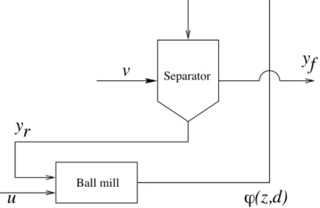
This paper is concerned with the feedback stabilization of industrial cement mills. A schematic lay-out of a typical cement milling circuit is shown in Fig.1. The plant is made up of the interconnection of a ball mill and a separator. The ball mill is fed with raw material (cement clinker). After grinding, the milled material is introduced in the separator where the finished product (i.e the particles that are small enough) is separated from the oversize particles (also called tailings) which are recycled to the ball mill.

Traditionally, the application of feedback control to cement mills is limited to monovariable classical PI regulation of the circulating load (the tailings flow rate) with either the feed flow rate or the separator speed as control action. Recently, linear multivariable control techniques have been introduced to improve the performances of the milling circuit (see e.g.[1], [2] and the references therein). However linear controllers based on a linear approximation of the process, are stable and effective only in a limited range around the nominal operating point. On some occasions, it is observed on real plants that intermittent disturbances (like for instance changes in the hardness of the raw material) may drive the mill to a region where the controller cannot stabilize the plant. This is well known by the operators as the so-called plugging phenomenon of ball mills.

In order to cope with this problem, a simple nonlinear model of the milling circuit has been presented in [4]. This model specifically includes the material hold-up (amount of material inside the mill) as a state variable. It is able to reproduce the plugging phenomenon in a realistic way.

∗_{This paper presents research results of the Belgiam Program on Interuniversity Attraction Poles, initiated by}

yr

yf

u

(z,d)

v

!

Figure 1: Schematic view of a milling circuit

In [4], an output feedback nonlinear predictive controller for this model is investigated. It appears that this controller has a larger stability region than the linear controller of [1] but can nevertheless not fully avoid mill plugging. The reason is that this controller does not use the material holdup which is essential to keep a global control of the process as also quoted in [5].

The contribution of the present paper is then to describe a state feedback nonlinear controller which includes a feedback of the material holdup such that the system has a single equilibrium semi-globally stable (and therefore globally attracting) in the domain of physical existence of the process. The controller is therefore able to completely prevent the mill from plugging. Moreover this controller is robust because it requires very little a priori knowledge of the plant (only the shapes of the grinding and separation functions need to be known).

2

Mathematical modelling

The following notations are introduced (see Fig.1). The mill is fed with cement clinker at a feeding rate u [tons/h]. The separator is driven by its rotational speed v [rpm]. The tailings are recycled at a rate yr [t/h] to the mill while the finished product exits the plant at a rate yf

[t/h]. The plant is described by a simple dynamical model with three state variables :

Tf˙yf = −yf + (1− α(v))ϕ(z, d) (1)

Tr˙yr = −yr+ α(v)ϕ(z, d) (2)

˙z = −ϕ(z, d) + yr+ u (3)

where Tf, Tr [h] are time constants, z [t] is the amount of material in the mill (also called the

mill load), d represents the clinker hardness, α(v) is the separation function and ϕ(z, d) is the ball mill outflow rate.

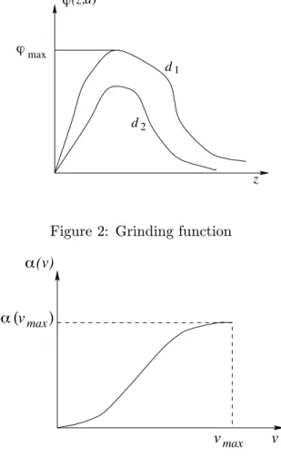
The grinding function ϕ(z, d) is shown in Fig.2 for different values of d. It is a non monotonic function of the mill load z. When z is too high, the grinding efficiency decreases and leads to the obstruction of the mill (plugging). A low value of z is also undesirable because it causes a fast wear of the balls.

d1 (z,d) d₂ max z ! !

Figure 2: Grinding function

v_max

v_max

" ( ) "(v)

v

Figure 3: Separation function

The separation function α(v), shown in Fig.3, is a monotonically increasing function of the rotational speed v of the separator, constrained between 0 and 1 with 0 ≤ v ≤ vmax and

α(vmax) < 1.

Of paramount importance is the fact that with this modelling of the grinding and separation functions, the system (1)-(2)-(3) is positive (see e.g. [3]) in accordance with the physical reality :

if yf(0)≥ 0, yr(0)≥ 0, z(0) ≥ 0, u(t) ≥ 0

and 0≤ v(t) ≤ vmax for all t≥ 0

then yf(t)≥ 0, yr(t)≥ 0 and z(t) ≥ 0 for all t ≥ 0.

Indeed, equations (1)-(2)-(3) show that whenever a component of the state becomes zero its derivative is non-negative.

3

Stability of equilibria

Assuming that the clinker hardness d is constant, the equilibria of the system ¯yf, ¯yr, ¯z are

parametrized by the constant inputs ¯u and ¯v : ¯ yf = ¯u (4) ¯ yr = α(¯v)¯u 1− α(¯v) (5) ϕ(¯z, d) = u¯ 1− α(¯v) (6)

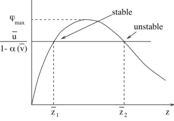
In view of the shape of ϕ(z, d) as illustrated in Fig.4, there may be zero, one or two equilibria. There are two distinct equilibria when the following inequality is satisfied :

¯

u < (1− α(¯v))ϕmax(d) (7)

where ϕmax(d) is the maximum value of the function ϕ(z, d) with respect to z. Linearizing the

model (1)-(2)-(3) at these equilibria, the eigenvalues satisfy :

λ1 = −Tf−1 (8)

λ2+ λ3 = −ϕz(¯z, d)− Tr−1 (9)

λ2λ3 = Tr−1ϕz(¯z, d)(1− α(¯v)) (10)

where ϕz denotes the partial derivative of ϕ with respect to z. From (9)-(10), we conclude

that the stability of the equilibria is determined by the sign of ϕz(¯z, d). The equilibrium is

exponentially stable if ϕz(¯z, d) > 0, whereas it is unstable if ϕz(¯z, d) < 0. In Fig.4, the stable

situation corresponds to equilibria to the left of the maximum of the curve, while unstable equilibria are located to the right of the maximum. When ϕz(¯z, d) = 0, one of the eigenvalues

is zero and the stability of the equilibrium is determined by the centre manifold dynamics :

˙z =−ϕ(z, d) + ¯u± ¯yr (11)

The equilibrium z = ¯z of (11) is unstable since (z− ¯z) ˙z > 0 for z%= ¯z.

4

The plugging phenomenon

The plugging phenomenon manifests itself under the form of a dramatic decrease of the produc-tion and an irreversible accumulaproduc-tion of material in the mill due to intermittent disturbances of the inflow rate and variations of clinker hardness. In the model (1)-(2)-(3) with constant inputs ¯

u and ¯v, plugging is a global instability which occurs as soon as the state (yf, yr, z) enters the

set Ω defined by the following inequalities (see Fig. 5) : yf ≥ 0, yr≥ 0, z≥ 0

(1− α(¯v))ϕ(z, d) < yf < ¯u

α(¯v)ϕ(z, d) < yr

z !( z,d) z z stable unstable ! 1- " (v) u 1 2 max

Figure 4: Equilibria and their stability

z y u f r y z 1#" ( ) " ! !

Figure 5: The plugging set Ω

Indeed, it is not difficult to observe that Ω is a positively invariant set and that in Ω : Tf˙yf < 0

Tr˙yr < 0

˙z > 0 Therefore we have that in Ω :

yf → 0, yr→ 0, z → ∞ as t → ∞ (12)

Hence the level z of material in the mill is accumulated without limitation while the production rate yf goes to zero.

5

Robust global stabilization

The control objective considered in this paper is to regulate the production rate y_f and the mill load z at desired set points y_f∗and z∗ by acting on the feed rate u and the separator speed v. The controller must prevent the mill from plugging and achieve global stabilization. Moreover, the controller must be robust against modelling uncertainties. More precisely our design only relies

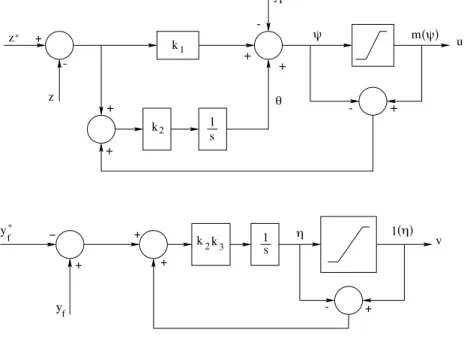
u 1 + + - + m($) % -yr -+ + $ s v (&) y + + f f 1 s & l + -* y z z * k k 1 2 # + + 2 k k₃

Figure 6: Block diagram of the controller

on the shape of the grinding function ϕ(z, d) and the separation function α(v) as illustrated in Fig. 2 and 3. No quantitative analytical model of these functions is assumed to be known.

The control inflow rate u and the control separation speed v are physically constrained to be positive and saturated. The control objective will be achieved with the following control law :

u = m(ψ) (13)

ψ = −yr+ k1(z∗− z) + θ (14)

˙θ = k2(z∗− z) + k2(m(ψ)− ψ) (15)

v = l(η) (16)

˙η = k3(k2(yf − y∗f) + k2(l(η)− η)) (17)

where m(ψ) = sat[0,umax](ψ) and l(η) = sat[0,vmax](η).

This is a very simple control law made up of two saturated PI controllers with anti wind-up and a ”feedforward” of yr into the z-regulator which decouples the two loops (see Fig.6).

The closed loop system (1)-(2)-(3)-(13)-(14)-(15)-(16)-(17) is then rewritten as

Tf˙yf = −yf+ (1− α(v))ϕ(z, d) (18) Tr˙yr = −yr+ α(v)ϕ(z, d) (19) ˙z = −ϕ(z, d) + yr+ m(ψ) (20) ˙θ = k2(z∗− z) + k2(m(ψ)− ψ) (21) ˙η = k3(k2(yf− yf∗) + k2(l(η)− η)) (22) ψ = −yr+ k1(z∗− z) + θ (23) v = l(η) (24)

In the next theorem, the stability properties of this closed loop system will be analyzed. Some technical notations must be introduced. The clinker hardness d is assumed to belong to an interval of admissible values [d1, d2]. For each value of d∈ [d1, d2], the grinding function ϕ(z, d)

as depicted in Fig.2 is a twice differentiable Lipshitz function of z, with a Lipschitz constant denoted k0(d). For each value of z ∈ IR+, ϕ(z, d) is a decreasing function of d. The maximal

value of ϕ is denoted

ϕmax = maxz∈IR+ϕ(z, d₁)

The separation function α(v) as represented in Fig.3 is also twice differentiable with :

α(0) = α$(0) = α$$(0) = α$(vmax) = α$$(vmax) = 0 (25)

We then have the following stability result where it is shown that the closed loop system has a unique equilibrium which is semi-globally stable in the domain of physical existence of the process.

Theorem

If d∈ [d1, d2], umax > ϕmax, k1> max(1, maxd∈[d1,d2]k0(d)), k3> 0

Then for any compact sets C(θ,η) ⊂ [−k1z∗,→ [×IR and C(yf,yr,z) ⊂ IR

3

+, there exists k∗2 > 0

such that for all 0 < k2 < k2∗ the single equilibrium of the closed loop system (18)-(24) is

asymptotically stable and its region of attraction contains C(yf,yr,z)× C(θ,η).

Proof

The domain A = {(yf, yr, z, θ, η)|yf ≥ 0, yr ≥ 0, z ≥ 0, θ ≥ −k1z∗, η ∈ IR} is invariant.

Indeed yr and yf are positive by nature, and z is positive by construction of the control law.

Moreover, if θ =−k1z∗, then ψ is necessarily negative and the control is saturated at zero, which

implies that

˙θ = k2((k1− 1)z + yr+ z∗) > 0 (26)

We may therefore assume that θ is initialized such that θ≥ −k1z∗ and restrict our attention to

the behaviour of the system inside the subdomainA.

The special case without integral action is first considered because it is the reduced-order model for a subsequent singular perturbation analysis.

Stability proof without integral action

Let us first consider the case without integral action (i.e. k2 = 0) and with the variables θ

and η fixed at arbitrary values ¯θ ≥ −k1z∗ and ¯η ∈ IR. The closed loop system

(18)-(19)-(20)-(21)-(22)-(23)-(24)reduces to Tf˙yf = −yf + (1− α(v))ϕ(z, d) (27) Tr˙yr = −yr+ α(v)ϕ(z, d) (28) ˙z = −ϕ(z, d) + yr+ m(ψ) (29) ψ = −yr+ k1(z∗− z) + ¯θ (30) v = l(¯η) (31)

Any equilibrium (¯yf, ¯yr, ¯z) must satisfy :

0 = −¯yf + (1− α(l(¯η)))ϕ(¯z, d) (32)

0 = −¯yr+ α(l(¯η))ϕ(¯z, d) (33)

0 = −ϕ(¯z, d) + ¯yr+ m(−¯yr+ k1(z∗− ¯z) + ¯θ) (34)

Eliminating ¯yr in (33) and (34), we obtain :

(α(l(¯η))− 1)ϕ(¯z, d) + m(−α(l(¯η))ϕ(¯z, d) + k1(z∗− ¯z) + ¯θ) = 0

This equation has no solution ¯z when (−α(l(¯η))ϕ(¯z, d) + k1(z∗− ¯z) + ¯θ) > 0 (because umax >

ϕmax) or < 0 (because this would require ¯z = 0, and the argument of m is ¯θ + k1z∗ > 0 when

¯

z = 0, which is a contradiction). Hence solutions must lie in the region without saturation and satisfy:

ϕ(¯z, d) + k1z = k¯ 1z∗+ ¯θ (35)

The left hand side is a monotonic increasing function of ¯z (because k1 > k0(d)) with value 0 at

¯

z = 0. The right hand side is strictly positive. Therefore this equation has a unique solution ¯

z > 0. The unique corresponding equilibrium values (¯yf, ¯yr) follow from (32)-(33).

We have just shown that a unique equilibrium exists for any value of ¯θ >−k1z∗ and ¯η∈ IR,

thus obtaining a family of equilibria (¯yf(¯θ, ¯η), ¯yr(¯θ, ¯η), ¯z(¯θ)) parametrized by ¯θ and ¯η.These

functions ¯yf(¯θ, ¯η), ¯yr(¯θ, ¯η) and ¯z(¯θ) areC2 because ϕ(z, d) and α(v) areC2 and because of (25).

We still have to show that the vector (¯yf(¯θ, ¯η), ¯yr(¯θ, ¯η), ¯z(¯θ)) is a GAS-LES equilibrium of

the system (27)-(28)-(29)-(30)-(31) for any fixed value of (¯θ, ¯η).

The system (27)-(28)-(29)-(30)-(31) is the cascade of the system (28)-(29)-(30)-(31) with the GES scalar subsystem :

Tf˙yf =−yf + (1− α(v))ϕ(z, d) (36)

We first show that the equilibrium of the subsystem (28)-(29)-(30)-(31) is GAS-LES for any (¯θ, ¯η). Let us select the constant c > 0 large enough such that

ψ =−yr− k1z + k1z∗+ ¯θ < 0

for all (yr, z) in the set

S ={(yr, z) : yr≥ 0, z ≥ 0, Tryr+ z = c}

Since ˙z + Tr˙yr < 0 when ψ < 0, the triangle T bounded by the coordinate axes and the straight

line S is invariant and globally attractive (see Fig. 7).

All the subsystem trajectories are bounded and reach T in finite time. The limit set of any trajectory inside T is either the equilibrium (¯yr(¯θ, ¯η), ¯z(¯θ)) or a limit cycle enclosing the

equi-librium. The segment of straight line joining the points (0, ¯z(¯θ)) and (¯yr(¯θ, ¯η), ¯z(¯θ)) is invariant.

Because any limit cycle should cross this segment, the only possible limit set is the equilibrium which is thus GAS. From the Jacobian linearization of the system the equilibrium is also LES.

y_r

$=umax

$=0

0 z z

S

Figure 7: Invariant triangle T

Now the equilibrium of equation (18) is GES when (yr, z) = (¯yr(¯θ, ¯η), ¯z(¯θ)). It follows from

Theorem A.1 in [8] that the whole subsystem (18)-(19)-(20)-(23)-(24) is GAS-LES. Stability proof with integral actions

We now come back to the case where k2 %= 0 and there is an integral action in the loop. We

will establish semiglobal stabilizability when θ and η are slowly varying. This can be achieved by taking k2 = ' small enough. With the change of time scale: τ = 't, the system is rewritten

in a two-time scale form as follows:

˙θ = z∗_{− z + m(ψ) − ψ (37)} ˙η = k3(yf − yf∗) + k3(l(η)− η) (38) 'Tf˙yf = −yf + (1− α(v))ϕ(z, d) (39) 'Tr˙yr = −yr+ α(l(η))ϕ(z, d) (40) ' ˙z = −ϕ(z, d) + yr+ m(ψ) (41) ψ = −yr+ k1(z∗− z) + θ (42)

The fast subsystem (39)-(40)-(41) is the system which has been analysed above, without integral action. When ' = 0, the fast variables are at their equilibrium (¯yf(θ, η), ¯yr(θ, η), ¯z(θ)). The slow

subsystem (37)-(38) then reduces to :

˙η = k3((1− α(l(η)))ϕ(¯z(θ), d)− yf∗+ l(η)− η) (43)

Because z can reach an equilibrium only when m(ψ) = ψ, equation (44) becomes: ˙θ = z∗_{− ¯z(θ) =} ϕ(¯z(θ), d)− θ

k1

(45) and the equilibrium θ = ϕ(z∗, d) of (45) is GES. Now, equation (43) with θ = ϕ(z∗, d) and z = ¯z(ϕ(z∗, d)) = z∗ (see equation (35)) is:

˙η = k3((1− α(l(η)))ϕ(z∗, d)− y∗f) + k3(l(η)− η)

This equation has a unique equilibrium η∗ verifying (1− α(l(η∗)))ϕ(z∗, d) = y∗_f and 0 < η∗ < vmax. It is easily seen that ˙η < 0 when η > η∗ and ˙η > 0 when η < η∗ and consequently that

the equilibrium η∗ is GAS-LES. It follows from Theorem A.1 in [8] that the equilibrium of the slow subsystem (37)-(38) is GAS-LES.

The proof is completed by applying the singular perturbation analysis of Theorem 3.18 in [6]. For any compact setsC(θ,η) ⊂ [−k1z∗,→ [×IR and C(yf,yr,z) ⊂ IR

3

+, there exists k∗2 > 0 such

that for all 0 < k2 < k∗2 the equilibrium of system (18)-(23) is asymptotically stable and its

region of attraction containsC(θ,η)× C(yf,yr,z). QED

6

Simulation results

The effectiveness of the proposed control law has been assessed through simulations where the model (1)-(3) represents the plant with analytical forms for the ϕ and α functions which satisfy the shape assumptions given in Sections 2 and 5 :

ϕ(z, d) = 20z exp(−dz 80) α(v) = 9( v vmax )3− 13.5( v vmax )4+ 5.4( v vmax )5 vmax= 200, αmax= 0.9

and the time constants Tf = 0.3 [h], Tr= 0.01 [h].

These functions have been tuned in order to match experimental step responses of an indus-trial cement grinding circuit (see [4]).

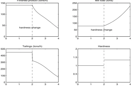
The plugging phenomenon is first illustrated in Fig. 8. The mill is initially running at a stable steady state ¯z = 78, ¯yf = 140, ¯yr = 448.4, ¯u = 140, ¯v = 141.5, d = 1 during the first

two hours. At time t = 2 hours, a small change of clincker hardness (d = 1.33) occurs. This disturbance produces plugging in the mill, as it can be seen in the figure, with an exponential unbounded accumulation of the mill load while the two other state variables tend to zero as expected.

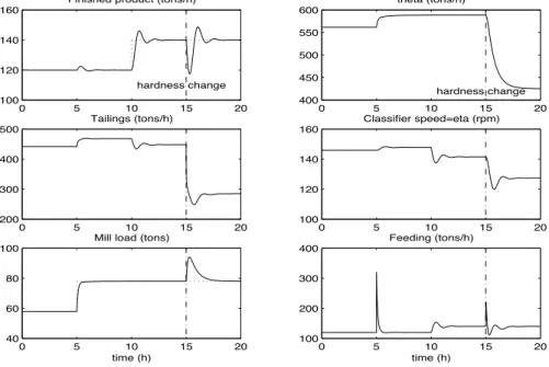
Various aspects of the closed loop behaviour are then illustrated in Fig. 9 with the design parameters set to k1 = 10, k2 = 10, k3 = 0.2. During the first six hours, the mill is at the

equilibrium with y∗_f = 120, z∗ = 58 and d = 1. A step change is then introduced on the mill load setpoint (z∗ = 78) at t = 5 hours. This is followed by a step change on the finished product setpoint (y_f∗ = 140)at t = 10 hours and by a hardness change (d = 1.33) at t = 15 hours. Note

0 1 2 3 4 0

50 100 150

Finished product (tons/h)

hardness change 0 1 2 3 4 0 50 100 150 200 250

Mill load (tons)

hardness change 0 1 2 3 4 0 100 200 300 400 500 Tailings (tons/h) 0 1 2 3 4 0 0.5 1 1.5 2 Hardness

Figure 8: The plugging phenomenon

that this hardness change is identical to that of Fig. 8 and would destabilize the mill in open loop. Furthermore, the same hardness change would also produce a destabilization of the LQG controller described in [1].

The following comments can be drawn from these figures.

1. The mill level is fairly well decoupled from finished product setpoint variations. This is mainly due to the feedforward compensation present in eq. (14).

2. The rejection of the hardness change disturbance by the mill load controller is very fast, which indeed prevents the mill from going into plugging. The effect of hardness changes on the finished product takes a longer time to disappear but it is also less critical since it does not destabilize the plant.

7

Conclusion

The goal of this paper was essentially to show that it is effectively possible to fully prevent industrial mills from plugging by state feedback, provided it includes the material holdup. In [5], the authors had also observed that this state variable is essential. Stability was therefore the main issue of the paper. Obviously, many other issues are interesting and should be investigated as for instance the limits of performance imposed by the stability requirement or the optimal selection of set points for productivity

0 5 10 15 20 100 120 140 160 hardness change Finished product (tons/h)

0 5 10 15 20 200 300 400 500 Tailings (tons/h) 0 5 10 15 20 40 60 80 100

Mill load (tons)

time (h) 0 5 10 15 20 400 450 500 550 600 hardness change theta (tons/h) 0 5 10 15 20 100 120 140 160 Classifier speed=eta (rpm) 0 5 10 15 20 100 200 300 400 Feeding (tons/h) time (h)

Figure 9: Simulation of the closed loop system

References

[1] Van Breusegem V., L. Chen, V. Werbrouck, G. Bastin and V. Wertz, “ Multivariable linear quadratic control of a cement mill : an industrial application”, Control Engineering Practice, vol. 2, pp. 605 - 611, 1994.

[2] Craig I.K. and I.M. MacLeod, ”Robust controller design and implementation for a run-of-mine ore milling circuit”, Control Engineering Practice, vol. 4, pp. 1-12, 1996.

[3] Luenberger D.G. ,Introduction to Dynamic Systems, Wiley, 1979.

[4] Magni, L., G. Bastin and V. Wertz, “ Multivariable nonlinear predictive control of cement mills”, IEEE Trans. on Control System Technology, Vol. 7(4), pp. 361 - 371, 1999.

[5] Boulvin M., C. Renotte, A. Vande Wouwer, M. Remy, L. Tarasiewics, P. C´esar, “ Modeling, simulation and evaluation of control loops for a cement grinding process”, Proceedings of European Control Conference (CD Rom), Brussels, July 97, paper TH-E-H4, 6 pages. [6] Sepulchre R., M. Jankovic and P. Kokotovic, ”Constructive Nonlinear Control”, Springer

Verlag, 1997.

[7] Vidyasagar M., ”Nonlinear Systems analysis”, Prentice Hall, 1993.

[8] F. Viel, F. Jadot and G. Bastin, ”Robust feedback stabilisation of chemical reactors”, IEEE Transactions on Automatic Control, Vol.42(4), 1997, pp. 473 - 481.