SIMREG, a tree-level distance-independent model
to simulate forest dynamics and management
from national forest inventory (NFI) data.
Jérôme Perin* (1), Mikhail Pitchugin (1), Jacques Hebert (1), Yves Brostaux (2), Philippe Lejeune (1), Gauthier Ligot (1)
(1) Forest Resources Management (GRF), Forest is Life, TERRA, Gembloux Agro-Bio Tech (GxABT), ULiège, 2 Passage des Déportés, 5030 Gembloux, Belgium
(2) Applied Statistics, Computer Science and Mathematics (SIMa), Gembloux Agro-Bio Tech (GxABT), University of Liege (ULG), 2 Passage des Déportés, 5030 Gembloux, Belgium
* Corresponding author at: Forest Resources Management (GRF), Forest is Life, TERRA, Gembloux Agro-Bio Tech (GxABT), ULiège, 2 Passage des Déportés, 5030 Gembloux, Belgium
Tel.: +32 81622295; fax: +32 81622301 E-mail address: j.perin@uliege.be (J. Perin)
Abstract
SIMREG is a non-deterministic tree-level distance independent forest model that can simulate forest growth, yield and management on a regional scale while representing the wide diversity of composition, structure and management found in forest stands. It is composed of several sub-models to represent the main forest dynamics (growth, recruitment, removal, clearcut and reforestation) and to account for species composition, stand density, tree size and social status, forest ownership type and some sites characteristics.
We used the data collected by the permanent forest inventory of Wallonia (IPRFW) between 1994 and 2015 to calibrate SIMREG and forecast the development of Wallonia’s 479 500 ha of productive forest (465 million simulated trees) until 2050. According to our simulation, the harvesting rate of Norway spruce (the main production species) is currently unsustainable and it is gradually being replaced by other species such as Douglas-fir, larch and various hardwoods. It appears that in terms of total softwood volume production, the higher production level of Douglas-fir and larch should eventually compensate for the decline in spruce. In contrast, the harvest rate in hardwood stands is around 75% of the annual yield, resulting in a steady increase in the total hardwood stock of about 600 000 m³ per year.
Our methodology is easily replicable and the data required for sub-model calibration are consistent with those measured by most permanent NFIs, so our forest simulation model could be adapted to other regions and countries.
Keywords:
Forest modelling; Individual tree models; Large scale simulation; Mixed forests; Forest growth and yield; Selective thinning; Tree recruitment
1. Introduction
The importance of forests cannot be overstated as they provide many critical economic, ecologic and social services such as wood production, climate change mitigation, soil protection and biodiversity habitats. It is therefore essential to have accurate and up-to-date information on the state of our forest habitats and a good understanding of forest dynamics (growth, harvesting, regeneration, etc.) to help implement sustainable forest policy.
Permanent forest inventory data remain the reference to estimate forest resources and dynamics (Barreiro et al. 2017). National Forest Inventories (NFIs) use statistical sampling methods to provide unbiased and accurate forest resources estimates from extensive sample plots inventory data. NFIs methodology varies greatly from one country to another (Vidal et al. 2016). The main methodological differences concern the spatial and time resolution of the sampling design, the sampling pattern (random vs systematic, single phase vs multi-phase), the plot characteristics (temporary vs permanent, angle gauged vs. circular, threshold diameter, etc), the data collected and the measurement techniques. While there is an increasing need for global reporting about forest resources (MacDicken 2015), much progress has yet to be made toward international NFIs harmonisation (Vidal et al. 2008; Baker et al. 2010).
At the European level, one of the most significant works in this direction is the recent implementation of the European Forestry Dynamics Model (EFDM) to harmonize forest resources projections until 2040 in 23 countries based on their respective NFIs data (Vauhkonen et al. 2018). EFDM is a stand level Markov chain model that simulates the development of forest area units defined by a collection of classifying factors according to probabilities of transitions (Vauhkonen and Packalen 2017).
Forest simulation models are increasingly being used to simulate forest dynamics and assess the likely impact of management choices (Taylor et al. 2008; Muys et al. 2010; Weiskittel et al. 2011; Burkhart and Tomé, 2012; Blanco et al. 2015; Blanco et al. 2020). Various modelling methods have been used which are usually categorized as empirical or mechanistic depending on whether the model components depict simple correlation or causal relationships (Twery and Weiskittel, 2013; Pretzsch et al. 2015). Empirical models are generally simpler to develop and apply than mechanistic models but their high dependency on the data used for parameterisation makes them mostly unsuitable for extrapolation to other systems or conditions (Vanclay 1994; Porté and Bartelink 2002; Taylor et al. 2008).
Models can also be classified depending on the spatial explicitness (distance independent vs distance dependent) and level (stand vs tree) at which the forest is modelled (Porté and Bartelink 2002; Pretzsch et al. 2015). Over the years, whole stand models have been successfully used in numerous studies to simulate forest succession and forest management on a large scale (e.g. Sallnäs 1990; Nabuurs et al. 2000; Vauhkonen et al. 2018). Their main appeal is their relative simplicity, making their calibration and operating much easier than for more data-intensive models. However, they lead to an evident loss of information about forest composition and structure which can be a relevant concern in the case of very diverse and heterogeneous mixed forests. On the other hand, generic large scale application of tree-level modelling approaches (e.g. Pretzsch 2002; Chertov et al., 2006; Huber et al. 2013; Stadelmann 2019) are generally very demanding in terms of data and computing power.
Tree level models are thus often highly specialized and aimed to assist understanding of natural processes and/or decision-making about local silvicultural management in specific forest compositions and structures (e.g. Valsta 1992; Courbaud et al. 2001; Le Moguédec 2011). A major interest of tree-level forest models is to allow the accurate simulation of the selective removal of trees (i.e. thinning). The significant impact of thinning on tree growth and forest stability, growing stock, carbon sequestration, etc. is well documented (e.g. Cameron 2002; Roberts and Harrington 2008; Schütz et al. 2015; Ruiz-Peinado et al. 2017). In temperate forests, selective thinning is broadly used as a tree-selection method to promote the growth response and stability of the remaining trees and is increasingly being promoted as an alternative harvesting strategy to shift from even-aged management to less intensive and more multifunctional forestry (Gamborg and Larsen 2002, Sterba and Ledermann 2006), As a results, it is critical to integrate detailed selective tree thinning procedures in forest models (Söderbergh and Ledermann 2003; Schmid et al. 2006; Petritsch et al. 2007, Mina et al. 2017).
In Belgium, forest management is a regional competence and each of the 3 regions (Wallonia, Flanders and Brussels-Capital) is responsible for its own forest inventory. About 77% of the total forest area is located in the southern region of Wallonia (Rondeux et al. 2010) and is monitored by the Permanent Regional Forest Inventory of Wallonia (IPRFW). The Walloon forests could be described as highly fragmented, heterogenous and intensively managed (Alderweireld et al. 2015). They are also undergoing rapid composition and structure changes to deal with recent forest disturbances, new environmental regulations and economic opportunities (Latte et al. 2016). As a result, questions are being raised about the sustainability of Walloon forest management and the future of sectors that depend on its wood supply. Moreover, available estimates of current growing stocks, yield and harvested volumes are often incomplete or even inconsistent because of several methodological discrepancies that have only recently been addressed (UNFCCC, 2020). For example, the last official IPRFW report (Alderweireld et al. 2015) provides regional estimates of harvested volumes exceeding production, which seems to contradict the increase in growing stocks observed over the same period.
Thus, there is a real interest in the development of a Walloon forest model to support IPRFW estimates and forecast the effect of changing forest management practices on the future of its wood stock, yield and supply in order to provide guidelines for policy makers, help improve our management plans and fulfil our internationals commitments (Global Forest Resources Assessment, National Forest Accounting Plan, Forest Reference Level, etc.). Such a model is also desired to help synchronise the IPRFW estimates with remote sensing data which would require that it operate with an annual step: a very convenient yet rather uncommon feature (Barreiro et al. 2017).
Moreover, the great diversity of composition, structure and management found in Walloon forests makes them an ideal case study to help develop and test a generic forest simulation tool. In view of the renewed interest for continuous cover forestry (Pommerening and Murphy 2004, Vitkova and Dhubháin 2013), it is of particular interest that such silvicultural approach is already well established in southern Belgium.
This study presents the forest model SIMREG and its application to assess the sustainability of the forest management currently applied in Wallonia. It focuses on the use of national forest inventories data to model forest management and its effect on the development of forest resources. SIMREG is designed as a multifunctional forest model to support research, assessment and management of forests at scales ranging from single forest stands to entire country. We intend to demonstrate that empirical tree-level distance-independent forest modelling approach based on NFIs data allow for an excellent compromise between usability, precision and performance by taking advantage of widely available data to achieve an optimal level of details while remaining applicable on a large scale. We also expect that it should help identify the main controlled factors that influence silvicultural practices such as selective thinning and thus enable accurate modelling of forest management at the tree level. With regard to our case study, we expect to confirm that the management of Norway spruce plantations is currently unsustainable, that the current reforestation trends are the main driver of forest change in Wallonia and that there are very significant management differences depending on the forest composition, structure and owner.
2. Material and methods
2.1. Study area
The study concerns Wallonia, the southern Region of the Kingdom of Belgium neighbouring France, Germany and Luxemburg. The Region is characterized by a Subatlantic climate, well-distributed rainfall throughout the year and altitudes ranging from 20 m in the western part (Western-Hainaut) to 700 m in the eastern part (Ardenne). Annual rainfall and mean annual temperature varies mostly according to the altitudinal gradient: from 800 mm and 10.5 °C in the west to 1400 mm and 7.5°C in the east (standards defined for the period 1981-2010 by the Royal Meteorology Institute).
Wallonia is divided in 5 contrasted ecoregions from north-west to south-east: Limoneuse region, Condroz, Famenne, Ardenne and Jurassic region. The Limoneuse region is a low-plateau (altitude of 100 to 200 m) of deep loess with a mild oceanic climate (annual rainfall of 850 mm, mean annual temperature of 10°C). The plateau of the Condroz alternate limestone and psammitic bedrock with a thinner loessic cover. The Famenne is a large depression with shallow and compact clay-shale soils. The former mountain range of the Ardennes is defined by its rough relief, up to an altitude of 700 m, on schisto-sandstone bedrock, rocky oligotrophic soils, with a submontane climate (1100 to 1400 mm, 8°C, the harshest climate of Wallonia). The Jurassic region presents a distinctive relief composed of cuestas, with relatively rich soils, and a more continental climate open to the south and protected by the Ardennes massif.
About one third (554 000 ha) of the Walloon Region is forest lands of which 479 500 ha are covered by productive forest area (Alderweireld et al. 2015). Most of Wallonia’s forests are located at the south of the river Meuse and in particular in the eastern natural region of the Ardenne where about 60% of the Walloon forest area is located.
The forest management applied in Walloon forest is generally rather intensive and most stands are regularly thinned. Significant differences in thinning intensities, rotations and reforestations are observed depending on forest composition, structure and the type of owner (Alderweireld et al. 2015; Latte et al. 2016). About half of the forest area is in the public domain and managed by the Department of Nature and Forests (DNF) of the Public Service of Wallonia (SPW). The other half is distributed among approximately 100 000 private owners, each of whom is responsible for the management of their own forest property.
Norway spruce (Picea abies (L.) H. Karst.) plantations are the dominant forest type in Wallonia: they represented around 34% of the total productive forest area, 41% of the standing stock and 53% of the total wood production in 2001 but have been in continuous decline since. Other softwoods stands represented around 12% of the total productive area and are mainly composed of pure plantations of douglas-fir (Pseudotsuga menziesii (Mirb.) Franco) and larches (Larix decidua Mill., Larix kaempferi (Lamb.) Carr. and Larix x eurolepis), mixed plantation of douglas-fir with Norway spruce and various forest stands dominated by scots pine (Pinus sylvestris L.).
About 54% of the productive forest area is occupied by hardwood stands dominated mainly by native oaks (Quercus robur L. and Quercus petraea (Matt.) Liebl.) and beech (Fagus sylvatica L.). In 2001, these two species represented respectively around 40 and 25% of the total hardwood standing stock. These two main species are often found mixed with various secondary species such as birch (Betula pendula Roth), ash (Fraxinus excelsior L.), hornbeam (Carpinus betulus L.) and maple (Acer pseudoplatanus L. and Acer platanoides L.) in a wide range of forest structures and compositions.
2.2. IPRFW data
Permanent sample plots (PSP) data were obtained from the Permanent Regional Forest Inventory of Wallonia (IPRFW) database. The sampling method applied by the IPRFW is presented in Rondeux et al. (2010), it is a single-phase, non-stratified inventory using a systematic sampling design with permanent sample plots at the intersections of a 1000 m (east-west) by 500 m (north-south) grid (each PSP thus represents 50 hectares or 0.5 km²). The PSP consists of three main concentric circular plots: trees with girth at breast height (Gbh) ≥ 120 cm are measured on the largest concentric plot (18 m radius), trees with 70 cm ≤ Gbh < 120 cm on the intermediate concentric plot (9 m radius) and trees with 20 cm ≤ Gbh < 70 cm on the smallest concentric plot (4.5 m radius). Therefore, the measured trees can represent different numbers of trees per hectare (called extension factor or Fext) depending on their Gbh.
A complete inventory cycle is divided into 10 equal independent shares called “tranche” according to a predefined scheme, ensuring that the whole territory is uniformly covered almost annually and that all site conditions and forest characteristics of Southern Belgium are represented. The first cycle of inventory was carried out between 1994 and 2008, the second is ongoing. We selected all data measured in permanent plots sampled between 1994 and 2015 that were representative of productive forest stands. This represent at total of 9 590 PSP of which half (= 5 tranches) were monitored twice at 6 to 16 years interval.
During this period, about 100 000 trees of 48 different species were measured. Most of these species are very marginally represented and have therefore been grouped in 3 miscellaneous classes, other very similar species of the same genus have also been grouped together (Table 6.1). This results in 11 broadleaves (hardwood, Hw) species groups: Native oaks, Beech, Birch, Ash, hybrid poplar (Populus spp.), Maple, Hornbeam, Black alder (Alnus glutinosa (L.) Gaertn.), Red oak (Quercus rubra L.), miscellaneous commercial hardwood (e.g. Prunus avium L. and Robinia pseudoacacia L.) and non-commercial broadleaves (e.g. Sorbus aucuparia L., Populus tremula L. and Salix sp.) and 6 conifers (softwood, Sw) species groups: Norway spruce, Douglas-fir, Scots pine, Larch, Black pine (Pinus nigra J.F. Arnold) and miscellaneous softwood (e.g. Picea sitchensis (Bong.) Carr. and Abies sp.).
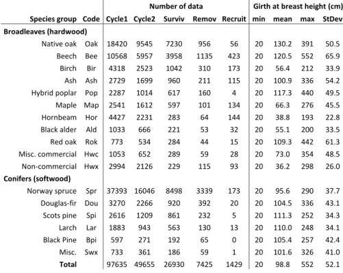
Table 6.1 Number and main attributes by species group of the tree measurement data obtained from the IPRFW. Cycle1 and Cycle2: number of trees measured during the first (complete, 1994-2008) and the second (in progress, 2008-2015) monitoring cycle. Surviv, Remov and Recruit: number of surviving, removed and recruited trees selected to model growth, thinning and recruitment.
Species group Code
Number of data Girth at breast height (cm) Cycle1 Cycle2 Surviv Remov Recruit min mean max StDev Broadleaves (hardwood)
Native oak Oak 18420 9545 7230 956 56 20 130.2 391 50.5 Beech Bee 10568 5957 3958 1135 423 20 120.5 552 65.9 Birch Bir 4318 2523 1042 310 173 20 56.4 212 33.9 Ash Ash 2729 1699 960 211 115 20 100.9 336 54.2 Hybrid poplar Pop 2287 1014 617 160 4 20 117.3 440 49.5 Maple Map 2541 1612 597 101 134 20 66.3 276 45.5 Hornbeam Hor 4427 2231 283 64 144 20 38.8 193 22.8 Black alder Ald 1033 666 221 53 32 20 55.1 200 33.5 Red oak Rok 773 534 284 44 15 20 109.3 442 61.3 Misc. commercial Hwc 1053 652 289 59 28 20 73.0 354 48.5 Non-commercial Hwx 2994 2126 229 115 93 20 36.2 298 26.0
Conifers (softwood)
Norway spruce Spr 37393 16046 8498 3339 173 20 95.6 290 37.7 Douglas-fir Dou 3270 2266 920 392 20 20 104.5 336 43.1 Scots pine Spi 2616 1209 861 232 5 20 111.3 252 34.3 Larch Lar 1883 943 563 130 13 20 110.0 248 34.1 Black Pine Bpi 597 271 192 65 0 20 105.4 257 42.4 Misc. Swx 733 361 186 59 1 20 101.6 326 41.0
Total 97635 49655 26930 7425 1429 20 98.8 552 52.1 1
The data needed to model growth, thinning and recruitment were selected from 3145 PSP monitored twice where at least one shared tree was measured in both sampling (to exclude clearcuts, new reforestations and displaced PSP). This represents 26 930 increments records from the trees that were measured twice, 7425 tree removals data from the trees measured in the first inventory but absent or dead at the second and 1429 tree recruitment data from trees that have exceeded the measurement threshold in the smallest concentric plot. The number and main characteristics of the measured data per species group are presented in Table 6.1.
2.3. Description of SIMREG
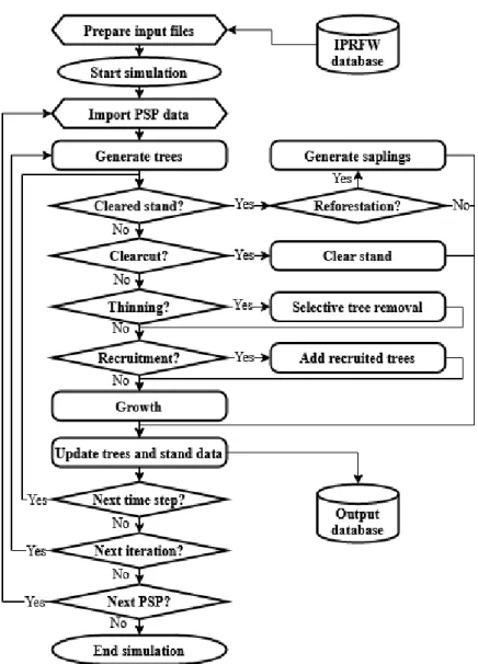
We developed a tree-level distance-independent forest simulation software (FSS) in the open software CAPSIS (Computer-Aided Projection of Strategies In Silviculture) simulation platform (Dufour-Kowalski et al. 2012). Each simulated forest stands is represented by a set of trees each with their own species and girth (circumference) at breast height (Cbh) and by a list of stand variables: simulated area, elevation, natural region, type of owner, etc. Various computation method are integrated to estimate the individual tree solid wood volume (volume of the stem and branches with a circumference exceeding 22 cm at smaller end) using the corresponding species-dependent taper models of Dagnelie et al. (1985) and calculate usual stand characteristics such as density, total basal area, volume and biomass per ha (Nha, Gha, Vha and BMha, respectively), mean and dominant Cbh (Cg and Cdom), etc. as well as continuous indicator of the stand composition and structure such as the proportion of each species group and the standard deviation of trees girth. The development of each virtual forest stands is simulated annually by applying stand-level clearcut and reforestation models and tree-level removal, growth and recruitment models (Figure 6.1). SIMREG currently does not account for any changing environmental factors as sub-models to estimate such effect on tree growth are still in development. Anyway, the present applications of our simulator focus on relatively short time scales (2000-2050) for which we assume that the influence of global changes should remain small compared to that of management.
We made it possible to directly use non-synchronized forest inventory data as input in our forest simulation software to easily generate a virtual forest stand. The inventory data are formatted in two input files: stands.inv and trees.inv. In stands.inv, each line represents a measured sample plot with its ID, type of owner, elevation, natural region, number and area (in ha) of virtual forests stands to be generated, simulation start and end year, rotation length and forest status at the start year (stocked forest stand or clearcut). In trees.inv, each line represents a measured tree with its corresponding sample plot ID, measurement year, species, Cbh and the number of trees it represent per hectare (Fext).
Each measured tree is then used to generate a number of virtual trees equal to Fext x stand area in hectare. In order to avoid generating thousands of identical trees, the girth of the generated trees follows a lognormal distribution of mean equal to the measured Cbh and of standard deviation equal to 5 cm. This amount of added noise was selected to be without consequences on the total standard deviation of the tree girth distribution in the virtual forest stand as it is roughly equivalent to the Bessel’s correction (So, 2008). This process can automatically be repeated any number of time so that 1) each sample plot can be used iteratively to generate several virtual forest stands and 2) the FSS can handle thousands of different sample plot inventories in sequence to generate a life-size forest resources representation at a regional scale.
Figure 6.1 Conceptual diagram of the forest model SIMREG.
The calibrated models are then applied sequentially each simulated years from the generation of a stand. First removal if in a rotation year (clearcut or thinning), then recruitment and finally growth which marks the transition to the following simulated year. Reforestation is a parallel process that is only applied in cleared (i.e. non-stocked) stands.
All of the necessary models were fitted in R (R Core Team, 2019) using stepwise methods, general linear and nonlinear regression procedure from the "nlme" package (Pinheiro et al., 2019) and survey-weighted general linear regression procedure from the “survey” package (Lumley et al., 2017). These models were then validated using a 5-fold cross-validation procedure (Kohavi, 1995). Models were fitted on 4 of the 5 tranches (training dataset) and then applied for the prediction of the remaining tranche (validation dataset). This was repeated 5 times to ensure that every tranche is used as validation dataset. This way, the validation mean error and validation root mean square error (or validation Brier score for logistic models) can respectively be used as estimator of the accuracy (unbiasedness) and precision (overall predictive performance) of the model when applied on an independent dataset. The direct comparison of the training and validation fitting statistics can also be used to assess the model adequacy as large differences would indicate under or overfitting.
The codes used in R to fit each model are presented in the supplementary material with the resulting fitting statistics, including the parameters t-tables. Only significant predictors variables were kept in these models but not all parameter values were significant at the factor-level. We decided not to arbitrarily restructure our level of factors (especially species groups) based on the significance of their parameter values.
2.4. Growth
The methodology used to model tree girth growth is based on the previous works of Deleuze et al. (2004) and Perin et al (2016). The original model is a distance-independent model that predict tree basal area annual increment using dominant height, dominant height annual increment, total basal area and tree girth as explanatory variable. However, significant adjustments had to be made to allow this model to be compatible with mixed irregular stands using only simple variables that are recoverable from most NFIs data. In particular, the use of age, dominant height and dominant height growth did not appear appropriate in uneven aged stands. Moreover, these variables were simply not always available in the IPRFW data and therefore needed to be substituted.
We found that the dominant girth was a suitable substitute for the dominant height and that most of the site effect on growth could be estimated from altitude alone in Wallonia. The resulting model is a 6 parameters (Aa, Ab, Pa, Pb, ma, mb) tree-level distance-independent species-dependent non-linear model that uses altitude (Alt), total basal area (Gha), dominant Cbh (Cdom) and individual tree Cbh (Ci) as explanatory variables to predict mean annual basal area growth (dGi):
dGi= 0.5 ∗ P ∗ (Ci− m ∗ A + √(m ∗ A + Ci)2− 4 ∗ A ∗ Ci) (Eq 1)
Where:
𝐴 = 𝐴𝑎 ∗ 𝐶𝑑𝑜𝑚𝐴𝑏 (Eq 1.1)
𝑃 = 𝑃𝑎 ∗ 𝑒𝑥𝑝 (1 − 𝑃𝑏 ∗ 𝐴𝑙𝑡) (Eq 1.2)
𝑚 = 1 + 𝑒𝑥𝑝 (𝑚𝑎 − 𝑚𝑏 ∗ 𝐺ℎ𝑎) (Eq 1.3)
The explanatory variables used (Gha, Cdom and Ci) are the averages between the first and the second inventory in order to represent the characteristics of trees and forest stands in the middle of the measurement period. In addition, the model was fitted on the mean annual girth increment value (dCi) rather than tree basal area growth segments (dGi) to avoid heteroscedasticity of residuals. To this end, the dGi estimated by the tree basal area growth model (Eq 3) were transformed in dCi using the following formula:
𝑑𝐶𝑖= (√𝐶𝑖2+ 4𝜋𝑑𝐺𝑖− 𝐶𝑖) (Eq 2)
We observed that the values of the parameters Ab and Pa were highly dependent on the species while the value of Aa, Pb, ma and mb varied very little within the hardwood and softwood division. We thus only fitted a division-dependent value for those five parameters to ensure the robust behavior of the model and ease the fitting convergence for the least represented species groups.
Annual growth is simulated by increasing the current girth value of each tree by its estimated increment. Stochastic effect is accounted for with random noise around the growth model estimates calibrated from the growth model residual distribution.
2.5. Removal
Removals refer to the trees that were removed by selective thinning or that died between two time frames (in our data, natural mortality account for about 5% of the total volume removed from the growing stock).
In a previous iteration of SIMREG, removals were simulated using a 2 steps process. The removal intensity was first estimated from stand characteristics and then trees were selected according to an individual score computed at the tree level. However, this method proved to be very compute intensive because of the large list of numbers that had to be sorted and difficult to calibrate for mixed stands. We thus decided to predict removal at the tree-level using a logit-function which make it much easier to account for the various stand composition and reduce total computation times by about 30%. This method has been used in few other forest models such as PrognAus (Ledermann 2006).
We used the data from the surviving and removed trees and formatted them in an Event/Trial format. The event is the removal and is either equal to 0 if the tree was still there and alive at the second monitoring or 1 if it was removed. The trial is the number of years that the tree existed between the two monitoring. For the surviving trees, it is simply equal to the duration in years between the two measurements (Period). However, we have to take into account that trees do not exist anymore after being removed. We assumed that on average, the removal took place exactly between the two inventories so that the number of trials is equal to Period/2 for removed trees.
We then calculated for each tree its annual proportion of event (= Event/Trial) and its weight corresponding to the number of “annual trees” it represent (= Trial x Fext). A survey-weighted generalised logistic procedure was applied using the svyglm() function (Lumley et al., 2017) on these formatted data to model the annual probability of removal. The variables considered were the species, girth and relative girth at the tree-level and the dominant girth, total basal area, standard deviation of the girth, proportion of each species, type of forest manager (private or public), elevation and natural region at the stand-level as well as their interaction up to the 3rd level.
The probability of removal was strongly related to the species and social status (relative size) of the tree and to the stand development stage and type of management (type of owner, density, structure). We identified and selected a subset of 7 relevant variables that had a significant influence on the probability of removals (Premovi), the formulation of the resulting logistic regression model is:
𝑃𝑟𝑒𝑚𝑜𝑣𝑖 = 𝑒𝑥𝑝 (𝑌𝑟𝑒𝑚𝑜𝑣𝑖) (1 + 𝑒𝑥𝑝(𝑌𝑟𝑒𝑚𝑜𝑣⁄ 𝑖)) (Eq 3)
Where:
𝑌𝑟𝑒𝑚𝑜𝑣𝑖= 𝑓(𝑆𝑝𝑖∗ 𝐶𝑟𝑒𝑙𝑖+ 𝑂𝑤𝑛𝑒𝑟 ∗ 𝐶𝑟𝑒𝑙𝑖+ 𝐷𝑖𝑣 ∗ 𝐶𝑉 ∗ 𝐶𝑟𝑒𝑙𝑖+ 𝐷𝑖𝑣 ∗ 𝐺ℎ𝑎 + 𝑝𝑐𝑔ℎ𝑎𝑠𝑝)
(Eq 3.1) Where: Spi is the tree species group and Div is the corresponding division (broadleaves or conifers); Owner is the type of owner (public or private); Creli is the relative girth (Ci/Cdom) of the tree; CV is the coefficient of variation of the tree girth distribution in the stand; Gha is the stand total basal area in m²/ha; pcghasp the proportion of the stand total basal area represented by the tree species group.
2.6. Recruitment
We modelled the recruitment density using a quasibinomial logistic regression approach to account for the singular distribution of the observed annual recruitment density value which range from 0 (80% of the PSP) to 304 trees per hectare. The recruitment data were formatted by dividing the observed annual recruitment density by 400 so that the recruitment model estimates the annual probability that a tree will exceed the inventory threshold in a 1/400th ha forest area. The variables considered were the dominant girth, total basal area, standard deviation of the girth, proportion of each species, type of forest manager (private or public), elevation and natural region as well as their interaction up to the 3rd level. We determined that the annual density of recruitment varied mostly with the structure and the density of the stand as well as some site related factors that appeared to be captured by the natural region. We identified and selected a subset of 4 relevant variables that had a significant influence on the annual recruitment density per hectare (Nharecrut), the formulation of the resulting model is:
𝑁ℎ𝑎𝑟𝑒𝑐𝑟𝑢𝑡 = 400 ∗ 𝑒𝑥𝑝 (𝑌𝑟𝑒𝑐𝑟𝑢𝑡) (1 + 𝑒𝑥𝑝(𝑌𝑟𝑒𝑐𝑟𝑢𝑡))⁄ (Eq 4)
Where:
𝑌𝑟𝑒𝑐𝑟𝑢𝑡 = 𝑓(𝑅𝑁 ∗ 𝐺ℎ𝑎 + 𝐶𝑔 + 𝐶𝑔2+ 𝐶𝑉) (Eq 4.1)
Where: RN is the natural region; Gha is the stand total basal area in m²/ha; Cg and CV are the quadratic mean and the coefficient of variation of the tree girth distribution in the stand.
We then modelled the recruitment composition according to the stand composition by averaging the recruitment composition observed in each PSP weighted by the corresponding total basal area proportion of each species-group found in the stand. First, we calculated for each PSP a recruitment vector (VRj) and a composition vector (VCj). The recruitment vector (VRj) is a row vector of length 17 where each value represents the recruitment density proportion (between 0 and 100 %) for each species group. The composition vector (VCj) is a column vector of length 17 where each value represents the stand basal area proportion (between 0 and 100 %) for each species group. We then multiplied the composition vector by the recruitment vector for each PSP, summed the matrixes obtained for all the PSP and divided the resulting matrix by the sum of the composition vectors (Eq 5):
∑(𝑉𝐶𝑗 𝑥 𝑉𝑅𝑗) ∑ 𝑉𝐶𝑗⁄ (Eq 5)
This results in a 17 x 17 matrix where each line represents the average composition of the recruitment density found below one species group. The vector of recruitment composition for a given stand composition can then be obtained by multiplying this 17 x 17 matrix by the column 1 x 17 stands composition vector.
In SIMREG, the recruitment density models is first applied to compute the total number of recruited trees in a virtual forest stand. The species of each recruited trees are then randomly selected according to the probability estimated using the recruitment composition model. The newly recruited trees are all generated in the virtual stand with a girth equal to the measurement threshold (20 cm).
2.7. Clearcut
We used aerial photographic interpretation to update the status of all the PSP in order to provide a more accurate assessment of the current resources of Wallonia (about 25 % of the sampled plots of the IPRFW were not monitored since 2000). Aerial photograph data (orthoimage) covering the whole Walloon Region territory were obtained from the Public Service of Wallonia (SPW) geoportal (http://geoportail.wallonie.be). These multispectral images (4 spectral bands: red, green, blue, and infrared) are characterized by a resolution of 25 cm and are available for the years 2006, 2009, 2012 and 2015. We then identified all the sample plots which have undergone a major transformation between their monitoring by the IPRFW and 2015 (e.g. clearcut and reforestation) using a specific application developed in the QGIS environment (GIS Opensource) and presented in Latte et al. (2015).
We modelled the probability of clearcutting using a binary logistic regression approach on the data obtained by photointerpretation. We selected the 6429 forest stands that were still standing on the orthophotos of 2006 from the 6921 productive forest stands sampled by the IPRFW before 2007. In this selection, 603 clearcuts were identified between 2006 and 2015. The data were ordered so that the status of every selected stand is represented each year from 2007 to 2015 by a 0 when the forest stand is standing and by a 1 when a clearcut was performed. A logistic binary regression was then performed on these data to estimate the yearly probability that a forest stand will be harvested depending on its characteristics. The variables considered were the dominant girth, total basal area, standard deviation of the girth, proportion of each species, type of forest manager (private or public), elevation and natural region as well as their interaction up to the 3rd level.
We identified the species composition, the development stage and the type of owner as the main predictors of the clearcut probability. We identified and selected 4 relevant combined variables that had a significant influence on the clearcut probability (Pcc), the formulation of the resulting logistic model is:
𝑃𝑐𝑐 = 𝑒𝑥𝑝 (𝑌𝑐𝑐) (1 + 𝑒𝑥𝑝(𝑌𝑐𝑐))⁄ (Eq 6)
Where:
𝑌𝑐𝑐 = 𝑓(𝑂𝑤𝑛𝑒𝑟 + 𝐶𝑑𝑜𝑚𝑥𝑆𝑊² + 𝐶𝑑𝑜𝑚𝑥𝑆𝑝𝑟² + 𝐶𝑑𝑜𝑚𝑥𝑃𝑜𝑝²) (Eq 6.1)
Where the Owner is the type of owner (public or private); CdomxSW², CdomxSpr² and CdomxPop² are variables obtained by multiplying the stand dominant girth (mean girth of the 100 biggest trees per hectare in cm) by the square of the proportion of the total basal area represented by respectively softwood, Norway spruce and hybrid poplar.
2.8. Reforestation
The data used to model reforestation were collected from the 475 newly reforested stand (212 in private forest and 263 in public forest) identified in this previous study. We worked in collaboration with the forest service of Wallonia (DNF) in public forest and with the IPRFW in private forest to retrieve more accurate information about the current species composition, structure and silvicultural objectives in the corresponding forest stands.
We assume the reforestation rate to be 100% in Wallonia as the total productive forest area is considered stable, with no significant change observed since the first inventory cycle. We analysed the data collected from 475 newly reforested stands to identify which variables had an influence on the composition of the reforestation and then model the probability of each type of reforestation depending on the characteristics of the previous forest stand.
Our simulator allows the configuration of a waiting period during which cleared stands stay non-stocked and no model is applied to account for the fact that reforestation are usually carried out several years after clearcuts. Once this period is completed, a simple random process is applied each simulated year to decide if any reforestation happens or if the stand stays non-stocked one more year. The composition and density of the reforestation is then randomly selected according to the probability defined in the reforestation model.
After analysis of the available data and consultation with forest experts, we have established the following elements: a) the waiting period and the subsequent annual probability of reforestation were set to 3 years and 50%, b) the girth assigned to each newly generated sapling follow a lognormal distribution of mean 1 and 0.5 of standard deviation and c) no removals and no recruitment happen until the dominant girth of the newly reforested trees first exceeds 40 cm. These parameters ensure that the average density and girth distribution obtained after 20 years of growth is equivalent to that measured in comparable stands by the IPRFW.
2.9. Simulation of Wallonia’s forest development
We initiated a simulation by generating virtual stands from the data of the first cycle of the IPRFW. While each PSP represents an area of 50 hectares, Southern Belgium forest stands are generally substantially smaller and we have chosen to use each PSP inventory to generate 10 virtual stands of 5 hectares (0.05 km²). The development of each virtual stand was simulated from the year its corresponding PSP was inventoried (1994-2008) until 2050. This means that the life-size representation of the Walloon forest is only achieved from the end of the first cycle of the IPRFW in 2008. We assumed that the total area of the Walloon productive forest and the type of owner of each virtual stand remained fixed during this period.
We have integrated thinning cycles into our simulator to take into account the resulting cyclical fluctuation of stand density. The first thinning year from the generation of each virtual stand is determined by an integer randomly generated between 0 and the rotation length minus 1, thinning and clearcut models are then applied every thinning cycle from this first date. The rotation length was set at 6 years for the following simulations. The annual probability are transformed into rotation probability using the following equation:
𝑃𝑅𝑜𝑡𝑎𝑡𝑖𝑜𝑛 = 1 − (1 − 𝑃𝐴𝑛𝑛𝑢𝑎𝑙)𝑅𝑜𝑡𝑎𝑡𝑖𝑜𝑛 (Eq 7)
3. Results
3.1. Growth models
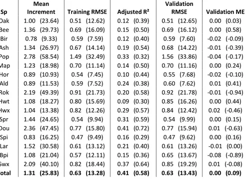
The calibrated model explains respectively 41% and 58% of the total variance on the annual girth and basal area increment. The performance of the model at the species-level is highly variable (Table 6.2) and the adjusted R² on the estimation of girth increment range from 9% for the miscellaneous commercial hardwood group to 41% for douglas-fir (respectively 30% and 72% on the basal area increment estimation). It appears to generally explain a larger part of the growth variability of faster growing species such as hybrid poplar, Norway spruce and douglas-fir. It seems reasonable to assume that a higher growth rate reduce the share in the total variance of the uncertainty caused by measurement inaccuracy and errors. These species are also found more often in even-aged plantations where the spatial distribution of trees is generally more homogenous and the effect of competition is therefore probably easier to estimate with a non-spatialized model.
Table 6.2 Observed mean annual growth and fitting statistics (RMSE = Root Mean Square Error, ME = Mean Error) of the parameterized growth model for each species groups; all statistics are presented for the annual tree girth increment estimation (cm/yr) and for the annual tree basal area increment estimation (cm²/yr, between parenthesis).
The analysis of the distribution of the validation residuals showed no evidence of bias over the entire range of each explanatory variable (individual tree girth, elevation, dominant girth and total basal area). We can also rule out under and overfitting as the training and validation RMSE values are also very similar for all the species group considered except black pine (Table 6.2). The relatively poor performance of the model for black pine is most certainly explained by its presence in only 21 different PSPs in our dataset.
3.2. Removals
The model shows that dominant trees (high Creli) generally have a lower probability of removals than dominated ones (low Creli), especially in private owned stands. However, the strong interaction between Crel and the standard deviation shows that this trend decreases in more irregular stands (high CV). This underlines that, in even-aged plantations, selective thinning is mostly applied to favor the growth of larger trees in preparation of the final harvest (clearcut) while in more irregular stands, trees that reach their logging dimension are regularly harvested to favor the natural regeneration (continuous cover forestry).
The calibrated parameters values reveal significantly different trends and removal rates between species (Table 6.3). For example, all other variables being equal, short rotation planted species such as douglas-fir and Norway spruce generally have a higher estimated removals probability than long revolution naturally regenerated species such as native oaks which are characterized by the lowest overall probability of removal. A notable exception to this rule is hybrid poplar that is generally planted at a very wide spacing and rarely thinned before the final harvest.
Sp
Mean
Increment Training RMSE Adjusted R²
Validation RMSE Validation ME Oak 1.00 (23.64) 0.51 (12.62) 0.12 (0.39) 0.51 (12.65) 0.00 (0.03) Bee 1.36 (29.73) 0.69 (16.09) 0.15 (0.50) 0.69 (16.12) 0.00 (0.58) Bir 0.78 (9.33) 0.59 (7.59) 0.12 (0.40) 0.59 (7.60) -0.02 (-0.09) Ash 1.34 (26.97) 0.67 (14.14) 0.19 (0.54) 0.68 (14.22) -0.01 (-0.39) Pop 2.78 (58.54) 1.49 (32.49) 0.33 (0.32) 1.56 (33.86) -0.04 (-0.17) Map 1.23 (18.98) 0.70 (11.14) 0.14 (0.50) 0.70 (11.16) 0.00 (0.24) Hor 0.89 (10.93) 0.54 (7.45) 0.10 (0.44) 0.55 (7.68) -0.02 (-0.10) Ald 0.89 (11.53) 0.59 (7.52) 0.24 (0.38) 0.60 (7.62) 0.01 (0.41) Rok 2.19 (49.39) 0.91 (21.73) 0.20 (0.58) 0.92 (21.78) -0.01 (-0.94) Hwt 1.08 (18.27) 0.80 (15.69) 0.09 (0.30) 0.85 (16.26) 0.00 (0.44) Hwx 1.04 (13.38) 0.82 (12.26) 0.29 (0.57) 0.84 (12.42) 0.02 (-0.46) Spr 1.44 (24.65) 0.54 (9.94) 0.31 (0.59) 0.54 (9.99) 0.00 (0.15) Dou 2.36 (47.45) 0.77 (15.80) 0.41 (0.72) 0.77 (15.94) 0.01 (-0.63) Spi 0.83 (16.25) 0.47 (9.49) 0.16 (0.29) 0.47 (9.62) 0.00 (0.16) Lar 1.52 (30.58) 0.61 (13.12) 0.21 (0.40) 0.61 (13.26) -0.01 (0.00) Bpi 1.08 (21.04) 0.57 (12.11) 0.15 (0.36) 0.65 (13.67) -0.08 (-0.89) Swx 2.09 (40.10) 0.82 (18.44) 0.37 (0.64) 0.85 (19.29) 0.01 (-0.08) Total 1.31 (25.83) 0.63 (13.28) 0.41 (0.58) 0.63 (13.43) 0.00 (0.09) 1
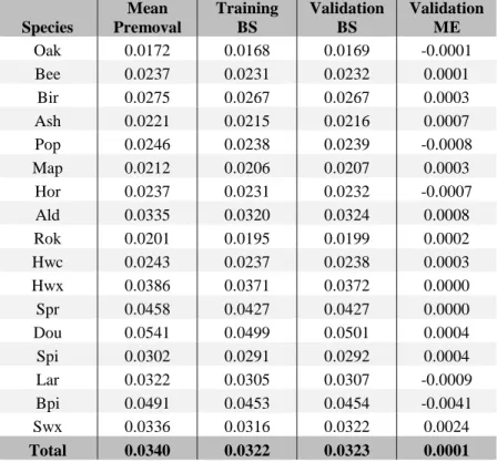
Table 6.3 Observed mean annual removal probability and fitting statistics (BS = Brier Score, ME = Mean Error) of the parameterized removal model for each species groups.
Species Mean Premoval Training BS Validation BS Validation ME Oak 0.0172 0.0168 0.0169 -0.0001 Bee 0.0237 0.0231 0.0232 0.0001 Bir 0.0275 0.0267 0.0267 0.0003 Ash 0.0221 0.0215 0.0216 0.0007 Pop 0.0246 0.0238 0.0239 -0.0008 Map 0.0212 0.0206 0.0207 0.0003 Hor 0.0237 0.0231 0.0232 -0.0007 Ald 0.0335 0.0320 0.0324 0.0008 Rok 0.0201 0.0195 0.0199 0.0002 Hwc 0.0243 0.0237 0.0238 0.0003 Hwx 0.0386 0.0371 0.0372 0.0000 Spr 0.0458 0.0427 0.0427 0.0000 Dou 0.0541 0.0499 0.0501 0.0004 Spi 0.0302 0.0291 0.0292 0.0004 Lar 0.0322 0.0305 0.0307 -0.0009 Bpi 0.0491 0.0453 0.0454 -0.0041 Swx 0.0336 0.0316 0.0322 0.0024 Total 0.0340 0.0322 0.0323 0.0001
Our model also shows an overall increase of the removal probability in denser stands (higher total basal area). However, this trend appears to be significantly weaker for coniferous species (for which a higher competition level is often recommended to avoid the formation of large branches).
The pcghasp variable makes it possible to differentiate in a stand between the dominant species (high pcghasp value) that generally are the main production objective and the dominated ones (low pcghasp value) that usually mostly have an accompanying role. Unsurprisingly, this variable shows that the main species generally have a higher probability of removals than accompanying ones also leading to a higher removal rate in monospecific forests.
Validation mean error (bias) are insignificant for all species group (Table 6.3) and the comparison between training and validation Brier score do not highlight any evidence of under or overfitting. The poor performance of the model for Black pine and miscellaneous softwood is probably due to the low number of PSPs in which these species are found in our data as well as the heterogeneity of the latter group of species.
3.3. Recruitment models
Recruitment data shows a large variability of which a significant part is likely random noise related to the small size (4.5 m radius) of the plot on which they are measured. Consequently, only a small part (Table 6.4) of this variability could be explained by our calibrated model even at it highlight some very significant relationships.
First, the polynomial relationship with the average tree girth (Cg) shows that the recruitment density decreases until around 120 cm of Cg and then increases again. It makes sense that the recruitment density is higher in very young forest stands that are more likely to already contain some trees whose girth is just below the measurement threshold and in very old forests where natural regeneration can sprout and develop. The parameterized model also indicates that the annual density of recruitment decreases with the total basal area (Gha) and increases with the dispersion of the tree girth (CV). This evidently shows that saplings thrive better in open irregular forest stands than in dense even-aged ones. We also found an interaction between the total basal area and the natural region. In particular, the negative effect of the
Gha on the recruitment density appears considerably higher in the harshest region of the Ardenne, probably due to greater competition for resources.
Validation mean error are insignificant for each natural region (Table 6.4) and the graphical analysis of the distribution of the validation residuals over the entire range of each continuous explanatory variable (Cg, Gha and CV) showed no evidence of bias. The comparison of the training and validation RMSE again shows no evidence of under or overfitting.
Table 6.4 Observed mean annual recruitment density and fitting statistics (RMSE = Root Mean Square Error, ME = Mean Error) of the parameterized recruitment model in each natural region.
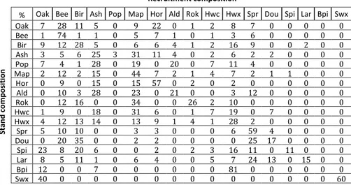
The recruitment composition model (Table 6.5) highlight some interesting trends that likely results from the very contrasted natural regeneration potential under continuous cover of the considered species groups. In particular, recruitments of native oaks appear very rare (except under scots pine), even in forest stands that it dominates where it is more likely to find recruitment of beech, hornbeam or birch. On the contrary, recruitments of beech appear very common under most forest composition but recruitment of other species is very rare under beech. Birch and beech are the only two deciduous species that recruit well under Norway spruce and douglas fir. Recruitments of ash and maple are often found together, sometimes in association with alder, hornbeam, poplar and/or miscellaneous hardwood. Norway spruce recruitments are common under itself, douglas-fir and larch with which it is often associated.
Table 6.5 Average recruitment composition (rounded to the nearest percent) according to the stand composition. Natural region Plot number Mean Nharecrut Training RMSE Adjusted R² Valid RMSE Valid ME Limoneuse 263 7.39 20.32 0.14 21.18 -0.28 Condroz 556 6.67 17.47 0.04 17.72 0.07 Famenne 432 5.76 14.48 0.09 14.70 -0.15 Ardenne 1662 6.81 21.31 0.21 21.81 0.04 Jurassique 232 11.85 23.18 0.14 23.57 -0.08 Total 3145 7.06 19.92 0.17 20.37 -0.02 1 Recruitment composition
% Oak Bee Bir Ash Pop Map Hor Ald Rok Hwc Hwx Spr Dou Spi Lar Bpi Swx
Stan d c o m p o si tion Oak 7 28 11 5 0 9 22 0 1 2 8 7 0 0 0 0 0 Bee 1 74 1 1 0 5 7 1 0 1 3 6 0 0 0 0 0 Bir 9 12 28 5 0 6 6 4 1 2 16 9 0 0 2 0 0 Ash 3 5 6 25 3 31 11 4 0 2 6 2 2 0 0 0 0 Pop 7 4 1 28 0 19 0 20 0 7 11 4 0 0 0 0 0 Map 2 12 2 15 0 44 7 2 1 4 7 2 1 1 0 0 0 Hor 0 9 0 15 0 15 57 0 2 0 2 0 0 0 0 0 0 Ald 0 10 3 28 0 23 0 21 0 0 3 12 0 0 0 0 0 Rok 0 12 16 0 0 34 0 0 26 2 10 0 0 0 0 0 0 Hwc 1 9 0 18 0 31 6 0 1 7 19 0 7 0 0 0 0 Hwx 4 12 13 14 0 13 9 1 4 1 28 2 0 0 0 0 0 Spr 5 10 10 0 0 3 3 0 0 0 6 59 4 0 0 0 0 Dou 0 20 35 0 0 2 2 0 0 0 0 25 17 0 0 0 0 Spi 23 8 20 6 0 0 2 0 2 3 16 11 0 11 0 0 0 Lar 8 5 11 1 0 6 4 0 0 5 7 24 13 0 15 0 0 Bpi 12 0 0 7 0 0 0 0 0 0 81 0 0 0 0 0 0 Swx 40 0 0 0 0 0 0 0 0 0 0 0 0 0 0 0 60 1
3.4. Clearcut probability models
The parameterized model shows that the probability of clearcutting is significantly higher in private owned stands than in public ones and increases with the dominant girth in forest stands composed of hybrid poplar and softwood and is consequently at its lowest in forests that contain neither (Figure 6.2). For a given dominant girth at breast height, the probability of clearcutting is the highest when Norway spruce is the dominant species, followed by hybrid poplar, then by the other softwood species (e.g. douglas-fir, pine, larch) and finally by other hardwood species where clearcuts are extremely rare.
Figure 6.2 Prediction in private and public forests of the annual probability of clearcutting as a function of the dominant circumference for 5 typical forest compositions: pure spruce (Spr), pure hybrid poplar (Pop); broadleaves without poplar (HW); conifers without Norway spruce (SW); mixed conifers with 50% of Norway spruce (SW+Spr).
3.5. Reforestation models
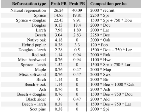
The reforestation data showed that the most important predictor of the reforestation composition and structure is the type of owner. In public and private forest, respectively 26% and 40% of all reforestations are achieved from natural regeneration. We observed that the composition of forest stands resulting from natural regeneration depended on the composition of the previous forest stand and appeared to follow the same pattern as the recruitment composition (Table 6.5). In the case of plantation, no relationship was found with the previous composition of the stand or any characteristics other than the type of owner. We identified 20 different plantation types and estimated their probability of implementation for each owner type (Table 6.6).
While the composition and density of natural regeneration is initially very variable, we found that it is generally quickly controlled by early silvicultural interventions in southern Belgium. We have observed that after about twenty years, the density and dimensions of trees in stands of similar compositions are usually comparable whether they are the result of natural regeneration or planting. Natural regeneration can therefore be effectively simulated by considering that it leads to reforestation densities equivalent to those of plantation (2000 trees per hectare on average) and that its composition follow the recruitment composition vector calculated just before the final harvest of the previous forest stand.
Table 6.6 Probability (in percent) associated with each observed type of reforestation depending on the owner type (PR = private and PB = public) and sorted in descending order of importance considering the total probability. The corresponding density per species group generated by the reforestation model are presented in the last column.
Reforestation type Prob PB Prob PR Composition per ha Natural regeneration 26.24 40.09 2000 * recruit
Spruce 14.83 19.81 2250 * Spr
Spruce + douglas 22.43 9.91 1500 * Spr + 750 * Dou
Douglas 9.13 18.4 2000 * Dou
Larch 7.98 1.89 2000 * Lar
Beech 3.04 2.83 2250 * Bee
Native oak 4.18 0 2000 * Oak
Hybrid poplar 0.38 3.3 120 * Pop
Douglas + larch 2.28 0.5 1500 * Dou + 750 * Lar
Red oak 1.14 0.94 2000 * Rok
Misc. hardwood 0.76 0.94 1100 * Hwc
Spruce + larch 1.52 0 1500 * Spr + 750 * Lar
Maple 0.76 0.47 2000 * Map
Misc. softwood 0.76 0.47 2000 * Swx
Birch 1.14 0 2000 * Bir
Beech + oak 1.14 0 1000 * Bee + 1000 * Oak
Ash 0.76 0 2000 * Ash
Beech + douglas 0.76 0 1500 * Bee + 750 * Dou
Black alder 0 0.47 2000 * Ald
Beech + larch 0.38 0 1500 * Bee + 750 * Lar
Scot pine 0.38 0 2000 * Spi
3.6. Simulation of Wallonia’s forest development
The entire productive forest resource of Wallonia generated from the first permanent inventory cycle made between 1994 and 2008 represent 479 500 ha of forest and about 465 million simulated trees distributed in 95 900 forest stands. Its simulation until 2050 required 54 minutes to complete on a computer equipped with an i9 7900x CPU (10 x 4.3 GHz) and 64 Go of RAM. The simulation outputs were stored in a 1,40 GB text file. We found that, given the large number of simulated trees (465 millions) and forest stands (95 900), no further replication was needed for the output values to converge. As the entire Walloon productive forest area is only simulated from the end of the first cycle of the permanent inventory (2008), the total solid wood stock estimates presented hereafter for the years 2000 to 2007 are extrapolated to the total surface area.
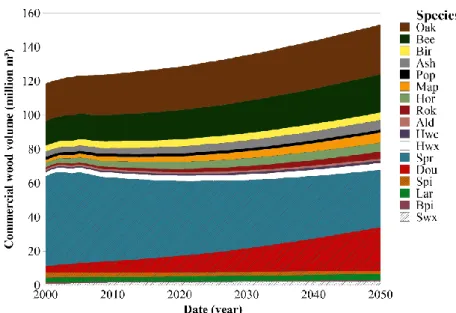
Our simulation shows a continuous hardwood stock increase of about 600 000 m³/year. Softwood stock would decrease until around 2020 and then would slowly recover: from around -300,000 m³/year in 2010 to +350,000 m³/year in 2050. There would be a substantial decrease in standing stock of Norway spruce and pines in favour of douglas-fir, larch and various hardwood species (Figure 6.3).
We plan an overall increase in the total wood production of the Walloon forest (Figure 6.4) mainly due to the gradual maturation of new plantations of fast growing species such as douglas-fir and larch. The hardwood production would also significantly rise because of a net increase of the share of hardwood dominated forest stands.
We observe (Figure 6.4) that the hardwood removal rate would remain relatively constant at respectively around 65% and 75% of the total annual hardwood production of private and public owned forests. Conversely, the current softwood management appears to be unsustainable (particularly in private owned forests) and we project that its removal rate should decrease in the coming decades. This is largely explained by the gradual replacement of Norway spruce which has a highly unsustainable removal rate of over 120% by other tree species with higher exploitable girth and lower removal rates such as douglas-fir and various hardwoods. In our simulation, this leads to a significant decrease of the total removal rate from 93% in 2010 to 83% in 2050. It appears likely that the removal rate of douglas-fir will eventually increase as it becomes one of Wallonia's main wood production species but this trends is not yet observed in the available inventory data.
Figure 6.3 Simulated development between 2000 and 2050 of the total growing solid wood stock (in millions m³) by species group.
Figure 6.4 Simulated development between 2009 and 2050 of the total annual wood production and removal (in millions m³) by division (SW = softwood, HW = hardwo od) and by type of owner.
4. Discussion
The trends highlighted by our simulation are consistent with previous reports about the observed changes of Wallonia’s forest resources. The most recent published estimates (UNFCCC, 2020) indicates an estimated solid wood stock increase of about 5 million m³ between 2001 and 2012 while our simulation estimated an increase of 5.01 million m³ over the same period. The current Norway spruce decline is also well documented (e.g. Hébert et al. 2002; Alderweireld et al. 2015) and is thought to have started following serious windfall damage in 1990 (Claessens 2006). In the same time, the better productivity, durability and resilience to windfall of douglas-fir and larches has made them the preferred alternative species (Pauwels 2003; Bievelet et al. 2007).
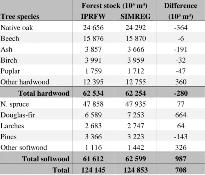
The total growing stocks per species predicted by SIMREG are reasonably close (within a one year variation) to the most recent estimates provided by the IPRFW (Table 6.7) except for a slight overestimation of douglas-fir growing stock. Although it may simply result from stochastic process, imprecision and the differences between the plots (whole network simulated vs half measured) and time periods (2012 vs 2008-2015) considered, it could also suggest that the current reforestation model is too optimistic in that it underestimates the share of douglas fir plantations that subsequently fail. It may therefore be worth collecting older data on reforestation in order to accurately estimate the success rate of plantations.
Table 6.7 Comparison of the estimates per species of the total growing stock from the first half of the second cycle of the IPRFW (2008-2015) with those of SIMREG for the year 2012.
Tree species
Forest stock (10³ m³) Difference (10³ m³) IPRFW SIMREG Native oak 24 656 24 292 -364 Beech 15 876 15 870 -6 Ash 3 857 3 666 -191 Birch 3 991 3 959 -32 Poplar 1 759 1 712 -47 Other hardwood 12 395 12 755 360 Total hardwood 62 534 62 254 -280 N. spruce 47 858 47 935 77 Douglas-fir 6 589 7 253 664 Larches 2 683 2 747 64 Pines 3 366 3 223 -143 Other softwood 1 116 1 442 326 Total softwood 61 612 62 599 987 Total 124 145 124 853 708
While individual tree models are generally considered more complex than stand-level ones, they are also more flexible (Pretzsch 2008) and streamline the representation of the potentially infinite range of forest stand compositions and structures (Pretzsch 2015). They also maximize the use of inventory data, both for model calibration and simulation initialization (Ledermann 2006; Stadelmann 2019). In SIMREG, the combination of this modelling approach with an annual simulation time-step makes it possible to directly use non-synchronized raw forest inventory data as input which should greatly facilitate its adaptation to other case studies. Moreover it also allows to synchronize IPRFW estimates with remote sensing and various survey data which opens interesting opportunities for forest assessment, management and research (Huang et al. 2018). We intend to continue to use this feature to regularly update the IPRFW data with external information such as those derived from the photointerpretation of clearcuts.
The performances of our growth model are comparable to those of other previously published empirical models (e.g. Monserud and Sterba 1996; Andreassen and Tomter 2003; Rohner et al. 2017). It is interesting to note that the validation RMSE on the estimated girth increment estimation for Norway spruce, douglas-fir and larches are almost identical to those obtained in a previous study (Perin et al, 2016) based on an entirely independent dataset: respectively 0.542 versus 0.545 cm/yr, 0.774 versus 0.771 cm/yr and 0.614 versus 0.627 cm/yr. However, the total annual girth increment variance in our dataset is comparatively lower for each of those species, leading to a lower adjusted coefficient of determination. This is certainly due to the over-representation in this previous study of data collected from several silvicultural field experiments representative of very unusual site condition and management practices.
Unsurprisingly, the explained share of the total annual girth increment variance is generally lower for species that are mainly found in mixed irregular stands. Modelling tree growth, removals and recruitment in mixed uneven-aged forests is undoubtedly complicated by the greater heterogeneity of local conditions (density, composition, structure…) compared to that of pure even-aged forests (Porté and Bartelink, 2002; Blanco et al. 2015). While distance-dependent approaches would have allowed to better account for local conditions (Pretzsch 2008), they require data that are not available in most forest inventory and would have been too compute-intensive for such large-scale applications. In the case of a regional forest management model, tree-level predictions need to be accurate (unbiased) but not overly precise so that we found it more efficient to simply emulate the local heterogeneity with a stochastic modelling approach.
The use of timber removal sub-models based on inventory data to emulate the behavior of forest owner is rather uncommon in large-scale forest models (Sterba et al. 2000; Söderbergh and Ledermann 2003; Thurnher et al. 2011; Barreiro et al. 2017). Nonetheless, the usefulness of analytical thinning algorithms to accurately reproduce stands dynamics has already been demonstrated (Sterba and Ledermann 2006; Mina et al. 2017). Our removal sub-model highlights many interesting trends depending on the composition, structure and type of owner which clearly demonstrates its interest in view of the current forest changes and shift towards more multifunctional forest management strategies (Gamborg and Larsen 2002, Vitkova and Dhubháin 2013). In particular, it appears essential to take into account the interactions between forest composition, structure and type of owner that can lead to very distinct forest management strategies. For example, thinning account for respectively 95% and 60% of the total volume of hardwood and softwood annually removed from Walloon public forests while those values drop to 75% and 30% in private forests. We therefore intend to regularly improve and update the removal sub-model to identify and account for potential behavioral responses to the ongoing forest resources changes.
Current reforestation trends are undoubtedly the main drivers of the ongoing composition changes in Walloon forests. In particular, the low replantation rate of Norway spruce combined with the very young age at which it is harvested in private forests are the obvious causes of its rapid decline. Consequently, the clearcut and reforestation sub-models are probably the most influential elements to accurately forecast the future characteristics of our forest resources. While our dataset did not allow us to identify any sites effect on these process, it appears probable that such relation exists. Particularly considering that some regulations were enacted (DNF, 1997) to prevent the plantation of some tree species in unsuitable sites (e.g. Norway spruce on white clays and peat soils) and help restore some natural habitat (e.g. Natura 2000 network). We will therefore continue to try to improve these sub-models as new data become available to improve the precision and accuracy of our simulations.
The main limitation of SIMREG stem from the empirical nature of its sub-models which currently constrains its application to the simulation of more original scenarios. We are currently working on the development of easily parameterizable removals, clearcut and reforestation sub-models to overcome these limitations and provide a flexible decision-support tool to assist forest management planning. In the near future, we also plan to improve SIMREG with several complementary sub-models to account for natural disturbances and changing environmental conditions.
5. Conclusion and perspectives
Our modelling approach proved appropriate to develop forest management models suitable for a wide range of forests characteristics using only variables that are available in the majority of forest inventories. Our growth, removals, recruitment, clearcut and reforestation sub-models account for the interactions between species composition, stand density, tree size, social status, some sites characteristics and the type of forest ownership to accurately predict forest management in a forest stand. Our forest model SIMREG was also optimized for large-scale applications and it allows the simulation of hundreds of millions of trees generated from generic national forest inventories (NFI) data. It is therefore an interesting tool for predicting forest resources changes on a regional scale in order to provide guidelines for policy makers and help improve forest management plans.