Spray pattern simulation model for standardisation of boom behaviour tests.

Aspects of Applied Biology 66, 2002 International advances in pesticides application

Spray Pattern Simulation Model for Standardisation of Boom

Behaviour Tests

By F LEBEAU, X BOUCHAT, R RUTER and M-F DESTAIN

Unité de Mécanique et Construction, Gembloux Agricultural University, 2 Passage des Déportés B-5030 Gembloux, Belgium

Summary

Simulation models of spray pattern are required for the dynamic behaviour assessment of sprayer booms. The reasons are their ease of use and their independence regarding variable operating conditions such as liquid properties and nozzle state, which interfere with the discrimination between various dynamic properties. Although such models have been developed for many decades, no international consensus has been reached on their use in a standardised test procedure. A consensual model is tested in the scope of standardisation specific needs. It uses ISO-5682/1 spray table measurements of the static distributions to compute three 2-D distribution at three heights using a filtered back-projection algorithm. These distributions are interpolated to generate a 3-D matrix of repartition at various heights. This 3-D matrix is used as nozzle distribution description in a dynamic distribution model where the dynamic distribution is computed as a summation of the static distribution at successive positions. The model kernel was found suitable to predict repartition under a moving boom.

Keywords: Dynamical repartition model, spray pattern, sprayer assessment

Introduction

Homogeneous spray distribution in field crop protection is required to achieve an optimal treatment efficiency. Many technical developments on crop sprayers are designed to improve the spray coverage homogeneity: pressure regulation based on forward speed, boom suspension, automatic slope correction, low drift nozzles, air assistance etc.. As a result, an increasing interest has arisen in the development of testing procedures to quantify the advantages of this kind of machinery. Sprayer tests can be divided in two categories; homologation and inspection tests. The former concerns the admission of new sprayers to the market while the latter aims to control the technical state of used sprayers. Most European countries have their own homologation criteria and inspection procedures. Dialogue between the different countries to develop common methodologies is supported by various EC (European Community) projects, and CEN standards are being developed. ISO standards are also developed and improved on a regular basis.

The relevant parameters to be measured are selected on the basis of their influence on spray repartition. For instance, parameters such as the nozzle spray pattern and flow (ISO 5682/1), the behaviour of the flow regulator (ISO 5682/3), are measured on dedicated experimental set-ups. Boom movements have also been known for years to have a major influence on spray

distribution and various experimental set-ups have been designed to evaluate their importance (Sinfort et al,1997; Ramon et al, 1997; de Jong et al., 2000, Tian & Zheng, 2000). The effect of boom movements on repartition has also been the subject of extensive research and different models have been developed by the same authors to predict repartition, taking into account these movements. These models are based on the assumption that the repartition caused by a moving nozzle can be approximated as the sum of static distributions at successive positions. Sinfort et al. (1997) tested such a model in a global sprayer distribution simulation method. Simulation errors were found but their origin was not identified. Ramon et al. (2000) validated a model using a theoretical distribution in one dimension, and found good agreement at very low speeds. Unfortunately the model was not tested using realistic boom movements. De Jong et al. (2000) compared measured distribution with modelled distribution including vertical and horizontal boom movements. They found that the accuracy level of the prediction was variable for different settings. One important parameter of these models is the spray distribution of the nozzle. Some of the models use theoretical Gaussian 2-D distribution fitted using 1-2-D spray distributions measured according to ISO 5682/1. 2-Direct measurement of the 2-D nozzle distribution is preferably needed to be included in dynamic repartition models to take into account the true shape of the nozzle repartition which may differ significantly from the theoretical. Measurement of this 2-D nozzle distribution implies to use particular experimental designs or especially algorithms. A set-up based on spray table measurements is described by Tian L. et al. (2000) to measure 2-D distribution. Holterman et al. (2000) proposed an algorithm to extrapolate the 2-D distribution from 1-D measurements. They showed on theoretical distributions that a set of distribution patterns obtained at different angular positions transformed by filtered back-projection algorithm give 2-D patterns sufficiently accurate for application in computer simulations.

The objective of this study is to present a model aimed at predicting the dynamic repartition of a given nozzle including speed and height variations, which occur continuously during field operation. In order to take into account the real nozzle characteristics, its 2-D repartition was deduced from measurements performed on a spray table (standard ISO 5682/1). The global validation of the model was performed on a laboratory testing machine simulating the movements of the nozzle in field conditions.

Materials and methods

Static distribution

When using a spray table equipped with a nozzle located at height z, the projection of the original distribution D(x,y) at a specific angle θ from the y axis and at a distance s from the origin corresponds to a Radon transform r(s,θ) as defined by Kak A. et al. (1988):

dxdy s y x y x D s r( , )=

∫ ∫

θ

θ

δ

θ

with δ the Dirac impulse that characterises the measuring system, a rectangular window which length is adapted to the filling rate of the gutters.

The reconstruction of the distribution D(x,y) implies to take the inverse Radon transform of the projections. This is made in two steps, firstly the transform is back projected and then filtered with a two dimensional ramp filter. The back projection operator B is defined as

∫

θ

θ

θ

This operator represents the accumulation of the projections that pass through the point (x,y). To cancel the blur effect caused by this accumulation, a ramp filter must be applied. In the presence of noise, the pass nature of the ramp filter leads to amplification of high-frequency noise, and consequently an additional low-pass filtering is necessary for noisy signals. The implementation of the back projection was conducted using the filtered back-projection algorithm “iradon.m” of the image processing toolbox of Matlab (Mathworks, release 12 2000). This function is performed on the matrix formed by the measured projections at different angles, which have to be specified. The function allows the selection of several filtering options. This selection is of particular importance, as the algorithm is known to be sensitive to the noise in the Radon transform, especially at the higher frequencies. The choice of the filter is a compromise between the reconstruction accuracy and the noise reduction.

The nozzle distribution was measured by using an automated spray table (Lebeau et al., 2001). This latter is constituted of 32, five-centimetre wide and 1.5 m long gutters. This test stand meets the ISO-5682/1 requirements but has the advantage of being equipped with strain gauge sensors for automatic measurement of the collected liquid volume in the 500 ml test tubes. This last property was useful to perform rapid and accurate measurements of the distribution. A special device was mounted on the boom to allow nozzle rotation by 3°45’ steps, allowing up to 48 measurements of the projections r(s,θ) of the 2-D distribution. The total angle of rotation was limited to 176°15’ for symmetry reasons. The nozzle was located at a constant height (z) during a measurement and could be adjusted in the 0 – 1.5 metre range. The pressure was measured using a Bourdon Sedeme E-913 0-10 bar pressure transducer. Tap water at 13° Celsius was used for the trials.

Preliminary tests and sensitivity analysis on theoretical distributions showed that 24 projections (repartition measurements) at 7°30’ interval were a good compromise between the test time (half a day) and the reconstruction regarding to the repeatability of the measurements, the resolution (50 mm spacing between the gutters) and the collected volume measurement accuracy (0.5%) of the spray table .

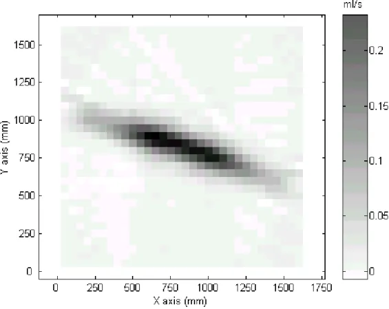
Measurements were performed on this spray table with a Teejet XR11003VK nozzle at 2 bar at 3 heights of 30, 50, 70 cm. The three sets of 24 projections were processed to compute the three 2-D flow distribution of the nozzle (ml/s) in a 32 by 32 grid of 50 mm wide square cells. Figure 1 presents a fake-grey image of the measured 2-D distribution at a nozzle height of 50 cm.

When comparing a mathematical projection on the x-axis of the reconstructed 2-D distribution with the original projection measurement on the same axis, differences were observed and over-estimation of the flow was found. This problem was solved by using zero-padding technique (Kak A. et al.,1988) using 32 lines of zeroes at each side of the measurements. Furthermore, spline interpolation and Ram-Lak filtration options were chosen (Mathworks). As the size of the table was limited to 1.5 m long and 1.6 m wide, the higher positions of the nozzle resulted in some losses. This effect affected the collected volume, especially when the main axis of the nozzle was in the direction of the gutters. To compensate for this effect, the total collected volume for each distribution was adjusted to the higher one by a proportional law applied on each gutter volume. Figure 2 shows that a good agreement with the original distribution was found, less than 1% deviation being observed.

Fig. 1. 2-D distribution of the flow output of a Teejet XR11003VK nozzle at 70 cm height.

Fig. 2. Comparison between the projection of the computed 2-D distribution and the corresponding original repartition measurement.

The distributions at the intermediate heights (between 30 and 70 cm) were interpolated while the distributions lower than 30 cm and higher than 70 cm were extrapolated using a scale factor based on a decreasing exponential law

( )

L(z): length of the sprayed surface at height z (m) Lmax: length of the sprayed surface at infinite height (m) b: constant parameter for a nozzle

The value of Lmax and b were computed by minimisation of the standard deviation between the 70 cm repartition and a rescaled 30 cm height repartition using the resize function with scale factor equal to L(70)/L(30) and the assumption that L(0,7)=1.6m. In our case, it resulted in Lmax =2.39 and b = 1.581. The distribution was then computed for every 5 cm between 0 and 2 m using this law. These results were re-sampled and stored in a standardised way within a 500*500*41 elements 3-D matrix. The matrix contained the value of the flow (ml/s) in every 25 mm² cells on a 6.25 m² square plane at 41 different heights between 0 and 2 m for every 5 cm height interval. This matrix D(x,y,z) was used as input to the dynamic repartition model.

Dynamic repartition model

The model is based on the assumption that the repartition must be a function of the time spent by the nozzle at each successive position, neglecting effects such as the release velocity of the droplets caused by the nozzle movement or atmospheric parameters. The axes x, y and z respectively correspond to forward, transverse and vertical direction (Fig. 3).

Fig. 3. Axis position.

Assuming that the motion according to y-axis is negligible, the time (t) when a nozzle is at a location (x,z) can be expressed as

) , ( zx g

t= (4)

Which can be estimated from distance and height measurements,

with x the absolute nozzle displacement along the travel direction and z the absolute height. Therefore, the amount of time δt spent in an increment δx at location (x,z) can be calculated by the partial derivative of equation (4)

( )

As the spray distribution is assumed to be constant for an uniform height z, the repartition caused in x and y by the nozzle at this height can be expressed by a convolution (denoted by * operator):

x

y z

∫

ξ

ξ

It appears that this convolution is strictly equivalent to a sum of static spray distribution D(x,y,z) at height z along the nozzle trajectory x for each successive position ξ proportionally to the time spent there by the nozzle (δt/δx)z. By analogy with linear system analysis, the distribution D(x,y,z) can be seen as the impulse response of the nozzle (measured using the spray table) while the trajectory of the nozzle along x axis, characterised by the partial derivative equation δg(x,z)/δx, represents the input signal of the system. As the impulse response of the nozzle was measured using a long time interval (typical measurement time was 120 seconds), it is a mean value of the nozzle characteristics. The rapid distribution variations, the pressure variations and long term evolution are therefore not taken into account by this linear, time invariant model.

The global repartition R(x,y) caused by the nozzle is expressed as the integral of the repartition for every height z

∫

In practice, the computation is performed on discrete distance intervals. Partial derivative is approached by a histogram for each successive height increment dz where the time spent in each space increment δx is computed. The choice of the step size is the result of a compromise between precision and the computational power required. Five mm wide steps were chosen, which is consistent with the repartition matrix. The sampling rate governs the number of samples in each interval that are used to estimate the partial derivative, in our case 1000 Hz. A low sampling rate limits the number of samples in each step, which ultimately leads to a binary function. To avoid this, a re-sampling of the signal at an appropriate frequency should be performed if acquisition rate is too low.

The main advantages of the model rely on the organisation of the computations that are optimised to take full advantage of the matrix calculation capabilities of Matlab, while the linear system description analogy opens a very broad field of specific mathematical tools for the system analysis and optimisation.

Experimental procedure for model validation

To validate the dynamic model, a special experimental set-up was used (figure 4). The device consisted of a boom section (1) mounted on a four-metre linear displacement table. The x-axis movement of the boom (2) is controlled by a computer and an electronic regulator in the ± 2 m/s range through a servomotor (3). It simulates the horizontal displacement of a sprayer boom. Any translation movement can be imposed within the available power limitations. Up to five nozzles can be mounted on the boom but only the central one (4) was used in this experimentation. The Teejet XR11003VK nozzle used for the static distribution measurements was mounted on the boom. A 0,3 % Nigrosine/water solution was sprayed at 2 bar. This dye was sprayed on 91.4 centimetres wide, 4 meter long laser grade white paper (5) lying on a table of adjustable height and slope (6).

Fig. 4. Experimental arrangement to validate the simulation model

The measurement of the collected deposits was performed at 100 dots per inch (dpi) using a A0 800 dpi feeder scanner. The processing of the resulting image was performed using image analysis software with a technique similar to the one proposed by Enfält (1997) who showed that this method was suitable for the assessment of the dynamic distribution. The liquid volume was measured in squares of 5 x 5 cm².

Results

Experimental results

Three movements of the Teejet XR11003VK nozzle were tested to validate the model. Test 1 was performed at uniform speed of 1 m/s and uniform height of 55 cm, test 2 at variable speed (1+0.565*cos (5,65t) m/s) and uniform height (55 cm) and test 3 at uniform speed (1m/ s) and height varying linearly from 70 to 30 cm in 3 m. Those movements were chosen on the basis of the analysis of the movements encountered in field trials and with respect to the capabilities of the experimental set-up. Table 1 presents a comparison of the simulation results with the dynamic measurements of the repartition.

Table 1. Comparison between measured and simulated dynamic distribution Test 1 (uniform speed

and height)

Test 2 (speed variation, uniform height)

Test 3 (uniform speed, height variation)

Meas. Simul. Meas. Simul. Meas. Simul.

Mean ml/m² 15.9 15.8 16 15.4 18.8 16.4

Max ml/m² 28 23.2 >40 >40 >40 36.2

Min ml/m² 6.3 6.8 3.7 4.4 1.9 1.7

CV % 27.5 33.4 49.7 50.2 42.2 41.4

R² 0.81 0.89 0.70

The results showed limited differences between modelled and measured distribution. For Test 1, most of the model errors are present in the transversal distribution. They were probably caused by the difference in the air flow over the repartition table and over the paper, the measured distribution being flattened. For test 2, the same problem is present. Longitudinal distribution was well predicted but further analysis suggests that the effect of the nozzle velocity at the spray release time is responsible of the remaining discrepancies. Correlation is better than for test 1 because variation are of greater amplitude. For test 3,

1 3 4 5 2 6

height variation effect was well predicted but errors increased as height diminished, mainly caused by entrained air effect on the deposition. Furthermore, the quality of the image analysis method showed limitation as dose-coverage relation appeared to be height dependant.

Discussion

A model was validated from the measurement of the static spray pattern to the dynamic repartition caused by realistic boom movement. The spray pattern simulation method proved to be an adequate tool to predict deposits under a moving boom. However, some limitations appear which should be taken into account when model choice is discussed for boom test standardisation in normalisation committees. Firstly, the static 2-D distribution is sensitive to collector configuration, essentially by its influence on the entrained air trajectory over the collection surface. Therefore, the measurement set-up geometry should be clearly defined. The choice of a reference method for 2-D static measurement should be based on a comparison of the existing methods with regard to their ability to be used as input in dynamic repartition models. Secondly, the dynamic model is adapted to predict the consequences of main boom movements on spray pattern but some improvements are possible. The height resolution of the 3-D matrix should be increased. Furthermore, the initial release velocity of the droplets or the wind effect could be taken into account. The increased quality of the prediction should be discussed with regard to the other sources of imprecision encountered in the field; such as variability and interaction between of the nozzles, pressure variations, and the target geometry.

References

de Jong E, Van de Zande J C, Stallinga H. 2000. The Effects of Vertical and Horizontal Boom Movements on the Uniformity of Spray Distribution. AgEng Paper 00-PM-015. Warwick.

Enfält P, Engqvist A, Alness K. 1997. Assessment of the Dynamic Spray Distribution on a Flat Surface Using Image Analysis. Aspects of applied Biology 48 : 17-24.

Holterman H J, de Jong A. 2000. Computing Static Two-Dimensional Patterns Using Patternator Observations. AgEng Poster 00-PM-067. Warwick.

ISO 5682/1. 1981. Matériel de traitement agropharmaceutique – Equipements de pulvérisation – Partie 1 : Méthodes d’essai des buses de pulvérisation. Norme Internationale.

ISO 5682/3. 1996. Matériel de protection des cultures – Equipements de pulvérisation – Partie 3 : Méthodes d’essai des systèmes de régulation du volume/hectare des pulvérisateurs agricoles à jet projeté. Norme Internationale.

Kak A C, Slaney M. 1988. Principles of Computerized Tomographic imaging. IEEE Press.. Lebeau F, Hamza E, Destain M F. 2001. Automatisation d’un banc de répartition pour

buses de pulverisation. Cahiers Agricultures. 9(6) : 505-509.

Mathworks. 1997. Image Processing Toolbox User’s Guide. The Mathworks, Inc. Natick, Massachussetts, USA

Ramon H, De Baerdemaker J. 1997. Spray Boom Motion and Spray Distribution : part 1, Derivation of a Mathematical Relation. J. agric. Engng Res. 66 : 23-29.

Sinfort C, Lardoux Y, Miralles A, Enfalt P, Alness K, Andersson S. 1997. Comparison Between Measurements and Predictions of Spray Pattern from a Moving Boom Sprayer. Aspects of Applied Biology, 48 : 1-8.

Tian L, Zheng J. 2000. Dynamic Deposition Pattern Simulation of Modulated Spraying Transactions of the ASAE. 43(1) : 5-11.