Does business abilities of the manager increase efficiency of incentive?

HAL Id: dumas-01074768

https://dumas.ccsd.cnrs.fr/dumas-01074768

Submitted on 15 Oct 2014

HAL is a multi-disciplinary open access

archive for the deposit and dissemination of

sci-entific research documents, whether they are

pub-lished or not. The documents may come from

L’archive ouverte pluridisciplinaire HAL, est

destinée au dépôt et à la diffusion de documents

scientifiques de niveau recherche, publiés ou non,

émanant des établissements d’enseignement et de

Does business abilities of the manager increase efficiency

of incentive?

Émilien Prost

To cite this version:

Émilien Prost. Does business abilities of the manager increase efficiency of incentive?. Economics and

Finance. 2014. �dumas-01074768�

Does business abilities of the manager increase

efficiency of incentive?

Emilien Prost, Université Lumière Lyon 2 GATE LSE

23/06/2014

Abstract

In this work, we intend to answer the question if ability of the manager increase efficiency of incentive. We first create a mathematical model on a principal-agent relationship. The assumption is to consider the performance of the manager as a source of legitimacy which is a factor that will change the tolerance to inequity of the agent. Two main prediction of this model are: 1) if the performance of the manager is lowers than the performance of the agent, every thing held equal the agent will decrease his effort. 2)if the performance of the manager is lowers than the performance of the agent, he will have to increase the piece rate he proposes in the contract to limit the negative impact of his illegitimacy on the agent effort. Then, we design and make an pilot experiment that attempt to observe in lab the first prediction of the model. Our preliminary results with a session of 14 participant are not statistically significant. However, they go in the direction of the theoretical model and could inspire us to perform other session.

Contents

1 Literature: Ability of manager as a source of legitimacy is a stake for authority and leadership issues 7

2 The model 9

2.1 The intrinsic motivation based on a illegitimacy aversion . . . 9 2.1.1 Defining illegitimacy aversion . . . 9 2.1.2 Properties of the illegitimacy aversion coefficient . . . 10 2.2 A principal-Agent model with no moral hazard and no risk aversion 11 2.2.1 Principal’s payoff function . . . 11 2.2.2 Employee’s payoff function . . . 11 2.2.3 The incentive constraint . . . 12 2.2.4 The principal maximization problem and the determination of

the equilibrium s∗ _{. . . . 13}

2.2.5 The determination of the equilibrium effort e∗ _{. . . . 14}

3 The Experimental design 15

3.1 Controlling qP and qAas exogenous parameters . . . 15

3.1.1 Tree stages: first stage with no principal-agent relationship will allow to make performance of all subject exogenous pa-rameter . . . 15 3.1.2 The task: finding the right balance between choosing a tasks

that allow legitimacy and avoiding learning effect. . . 16 3.1.3 Demand effect: do not draw subject’s attention to the

legiti-macy issue . . . 17 3.1.4 Choosing remuneration and resolving the issue of wealth effect

(a revoir avec le random sur stage 2 et 3) . . . 17 3.2 Session . . . 18

4 Result 19

4.1 Data . . . 20 4.2 Econometrics model: unobserved heterogeneity and endogeneity issues 21 4.2.1 Endogeneity . . . 21 4.2.2 Unobserved heterogeneity . . . 23 4.2.3 Fixed effect and random effect model . . . 23

Introduction

What happens very often in firm and organization, is that the manager before he became manager was previously a regular employee. And the current employee knows that in the past his supervisor used to perform the same task than he does himself now. He also knows that his supervisor had to work very hard and be technically competent to squeeze out competitors and finally become manager. Intuitively, this fact seems to give a lot of authority and legitimacy to the manager, so then, the agent is inclined to accept orders. This is a particular case of merit-based promotion system when the appropriate mea-sure of deservingness is business abilities. Business abilities are the technical knowledges of the job. And this technical knowledges become in certain firm the main criteria of selection of leaders as opposed to management skills or others criteria such as diplomas or network.

So the question that business ability of the manager could increase the efficiency of incentive is directly related to that. We choose to study the impact on intrinsic motivation. In terms of behavioral economics and contract theory the question would be to study if the illegitimacy of the principal could have a negative impact on the intrinsic motivation of the agent. In other words does the agent think it’s unfair to have a principal who has less business abilities that he has himself? In that case will he “make his own justice” by decreasing his effort?

This issue is related the literature on leadership, authority, legitimacy and to the literature on Peter Principle. Our work position it self in behavioral economics and human resources economics. To answer properly to the question it is important to distinguish the multiplicity of interpretations carried by the expressions "authority","legitimacy"and "incentive". First, "incentive" in common language is all of kind external reward such as money, help or external sanction. In our analyze we will focus on basic monetary incentive. Secondly, we use "business ability" as opposed to management skills. Because we try to analyze in what case business skill is key factor for general management ability which would be secondarily based on "pure" management skills like listening skills, general knowledge and vision etc... Why? Because if the agent has indeed a concern for legitimacy then, business abilities would impact the key means of management which are incentives. Thirdly, in the common knowledge, the word authority is derived from the Latin word auctoritas, meaning invention, advice, opinion, influence, or command. In English, the word authority can be used to mean power given by the state (in the form of Members of Parliament, judges, police officers, etc.) or by academic knowledge of an area (someone can be an authority on a subject). That refers to the Rational-legal authority describe by Max Weber in sociology. There are then two aspect of authority. One aspect is the direct power to influence the behavior of other. This power can be given by institution, by

vote, by political organization. This kind of authority refers to a claim of legitimacy, the justification and right to exercise that power. But it is mostly a certain type of formal relationship between one man or group and other people. The second aspect of the definition is the intellectual and moral authority or the informal authority of leadership. Here, the authority becomes not a formal relationship but an informal influence based on capacity. This second aspect could also become actually a source of legitimacy for formal authority. In our work we will focus on this kind of authority.

Finally, we will considered "legitimacy" of the manager as the fact that his business ability is superior to the ability of the agent. There are of course others sources of legitimacy but we won’t take them in account in our work. So in this case, the question is how the agent compares is own ability with the ability of the principal and how it will have an impact on his intrinsic motivation.

In management science, the ability of the superior has a potential incentive reinforcer refers to the theory of transactional leadership which is relevant to describe supervisor more than executive managers. Indeed, in the transactional leadership, the leader must focus on the daily relationship with the followers and adapt his style to them. For example, they need to give them encouragement, reward, self confidence, training and direction [Van Wart, 2013]

The problem of legitimacy have been also studied in psychology. In 1975 Michener and Burt studied how legitimacy could determine compliance. They include in their variables, normativity, coercive power, collective justification but they do not include abilities or performance variables [Andrew and Burt, 1975]. In 2010, a problem close to legitimacy has been studied by Jong and Schalk who studied the impact of fairness on behavior [Jong and Schalk, 2010]. Indeed, they studied how extrinsic motivation can moderate the impact of perception of unfairness on employee outcomes. Except that the outcome was not the actual effort of the employee but his intention to quit, or his affective com-mitment or perceive performance. They made a survey and give a questionnaire to people to measure the fairness perception. Most questions were about fair reward and fair orga-nizational changes. Applying the logic of Schalk an Jong [Jong and Schalk, 2010]in the Principal-Agent framework, we could wonder if an increase of incentive could moderate the impact of a perception of unfairness due to the manager illegitimacy and more specif-ically on his business ability. In other words, it would mean that illegitimacy could cancel in part the impact of incentive on effort by decreasing the intrinsic motivation.

In economics, Schnedler, Wendelin and Vadovic, Radovan have studied in 2011 how negative response to control disappear when the principal is legitimate. They conjecture that control is legitimate when it is not aimed to a single agent, or if it protect the endowment of the principal [Schnedler and Vadovic, 2011]. Thus it is very different than

our work.

Indeed, our subject is strongly related to the the literature on procedural justice and distributive justice in social psychology and economics. First research on justice focused on people’s feelings and behaviors in social interactions flow from their assessments of the fairness of their outcomes when dealing with others (distributive fairness). John Thibaut and Laurens Walker study the impact of “procedures” as opposed to “distribu-tive”justice based on outcome. Procedures was here considered as the mechanism to allocate outcomes[Thibaut and Walker, 1975]. This idea was developed more recently in psychology by Tyler and Blader in 2003[Tyler and Blader, 2003] or in economics by Ku and Salmon [Ku and Salmon, 2013]. The contribution of our work is to use to use the contract theory framework and study want could be the strategic behavior taking into account the aversion to illegitimacy. In our case, selection of leaders based on their busi-ness abilities would be a particular case of procedure. Aversion to illegitimacy would be interpreted as a concern for a specific form of procedural fairness.

In our model we will considered legitimacy such as a factor of tolerance to inequity. That’s why our model is inspired by the model of inequity aversion of Fehr and Schmidt , the model of Englmaier and Wambach in 2010 , and the model of Vital Anderhub, Simon Gachter and Manfred Konigstein and it is focused on the idiosyncratic parameter of their model.

In their model they assume that the intrinsic motivation of agent is function of the spread of income with the principal. The weight of this spread on the global payoff is a idiosyncratic parameter of their model. It is the individual tolerance to inequity. Then in our work we assume this parameter is no longer idiosyncratic but varies according to the relative ability of the principal compare to the ability of the agent. Thus, the sensitivity of the agent to inequity increase with illegitimacy of the principal. We make the assumption is that illegitimacy is not a problem in itself, but the agent start to have a concern about this when there is inequity. So legitimacy becomes a sharing criterion of collective gains. Eventually, we have an experimental approach because this fit in the literature of fairness and we expect some result. We made a pilot experiment with 14 participant. Our preliminary result are statically significant but go in the same direction than the model. This is an incentive to perform other session.

The two main prediction of our model are:

1- if the principal has no legitimacy, and the inequity of payoff is in favor of the principal, every thing held equal the agent will decrease his effort.

2- the principal with no legitimacy will have to increase the piece rate he proposes in the contract to limit the negative impact of his illegitimacy on the agent effort.

In the first part, we will study that considering "business ability" as a potential incentive reinforcer follows previous research about authority, legitimacy, leadership and incentive and how legitimacy is a stake. In the second part, we will explain our model. In the third part we will describe our experimental design. In the fourth part, we will explain our result from our pilot experiment.

1

Literature: Ability of manager as a source of

legiti-macy is a stake for authority and leadership issues

Our work is also related to the litterature on leadership. Some author wrote also about the utility of a leader. Benjamin E.Hermalin developed in 1998 the concept of leading-by-example [Hermalin, 1998]. The idea of the paper is to focus the analyze on a team who the principal/leader belong to. The employees rationally realize that the leader has a incentive to tell the employees that all activities deserve their fullest effort. Then the leader has to find a way to convince employee to work more on a specific task which will be to spend himself several hours working on this task. He shows the example. Jan Potters, Martin Sefton, Lise Vesterlund developed a similar idea and show that in an experiment of an endogenous sequential public game, the contribution is generally better than when the choice is simultaneous because of a following behavior [Potters et al., 2005]. Besides, Emrah Arbak and Marie Claire Villeval showed in 2011 that randomly chosen leaders are not less influential than voluntary leaders [Arbak and Villeval, 2007].

In economic literature: authority has been studied from formal relationship aspect and dilution of power but not from the aspect of legitimacy and competence.

Reichman and Rohling-Bastian study the fact that they are three components of an incentive system (i.e., performance measurement, rewards, and the allocation of decision rights). In practice, the authority to decide on these components is frequently distributed across hierarchical levels, thus requiring to adjust centralized decisions with regard to decentralized authority. They investigates the centralized design of incentive contracts when decision authority with respect to the allocation of tasks is delegated to lower hierarchical levels. It provides an analysis of the optimal allocation of authority (who should be the boss?) and considers the interdependencies between organizational design choices and the design of optimal incentives [Reichmann and Rohlfing-Bastian, 2013].

Aghion and Tirole distinguished between different types of authority with respect to the right to decide and effective control over decisions the distinction arises because of information asymmetry between the contracting parties. It is usually assumed that the principal fully retains the right to decide, whereas the agents have effective control [Aghion and Tirole, 1997].

Wulf analyzes the impact of division managers authority on incentives and finds a significant positive relation. Most notably, she finds that the pay-to-performance sensi-tivity for global performance measures (firm sales growth) is four times higher for division managers with more authority (measured by officer status) compared to those with less authority. However, she does not find a significant relation with respect to local measures [Wulf, 2007].

Theoretical literature has considered cases in which the principal cannot or will not retain full authority. Melurnad and Reichelstein consider a case of complete delegation [Melumad et al., ], i.e. the contract design and the task assignment are delegated to agents, and derive conditions under which the principal does not incur a loss from del-egation. Moreover, previous literature has shown that when relaxing the assumptions of the Revelation Principle, decentralization can be optimal for the principal. Benefits from decentralization then could arise from reducing costly communication and contract complexity [Laffont and Martimort, 1998].

Authority as been studied in economics mostly in the delegation of power aspect and decision right aspect. Our work is different. Indeed, as soon as we want to focus on issues about incentives and transactional leadership, we will work on the intellectual, moral and informal authority of leadership. This authority and leadership may be based on competence, the legitimacy and the respect associated with it.

In 2011, Schnedler, Wendelin and Vadovic, Radovan conjecture that control is legiti-mate when it is not aimed to a single agent, or if it protect the endowment of the principal . Legitimacy as been also studied in its democratic aspect [Vollan et al., 2013]. Vollan and Zoo shows that the efficiency of political institutions (democracy and authoritarian norms) depends on social norms.

In our work we are not focus on control or democratic issues but on competence as a source of legitimacy that could enhance tolerance to inequity. That lead us to another literature. The literature on justice and fairness. Initially it has been studied by social psychology [Thibaut and Walker, 1975]. Economist got interested in that but mostly stayed focused on “distributive fairness” which is behind the concept of “aversion to inequity” [Fehr and Schmidt, 2000]. Our work is related to psychological concept of “procedural fairness” which as been studied in psychology [Tyler and Blader, 2003] but is very less studied in economics [Ku and Salmon, 2013]. Procedures was considered as the mechanism to allocate outcomes. Our contribution is to use the framework of principal-agent theory and intend to construct a mathematical model that could give us prediction on the strategic behavior for the agent and the principal. In our case, the selection of the leaders by their business abilities becomes a specific “procedure” that could be interpreted as “unfair” and then decrease effort of the agent.

2

The model

To analyze the impact of illegitimacy on intrinsic motivation UA we will use a model

inspired to the model of inequity aversion of Fehr and Schmidt , the model of Englmaier and Wambach in 2010 . In our model, both agent and principal are risk neutral and the effort is contractible. We assume that illegitimacy is based on a comparison of relative performance between the agent and the principal. The legitimacy is related to business abilities and not on management abilities. It leads us to define I as a coefficient of aversion to illegitimacy. The main assumptions and limits of the model are:

• The agent and principal are risk neutral, there is no moral hazard, • There is perfect of information about preferences and performances, • The relative performance between agent and principal is exogenous, • There is one task: just the business abilities and no management abilities, • There is one period

2.1

The intrinsic motivation based on a illegitimacy aversion

2.1.1 Defining illegitimacy aversion

Definition. We define I as a coefficient of aversion to illegitimacy such that:

I(λ, qA, qP) = λ

qA

qP+ qA

(2.1) In this equation qAis the performance of the agent that the principal can observe and

qPis the performance of the principal. In that case, the agent can observe the performance

qPof the principal. We have defined qP and qAas a parameter in the model. The principal

and the agent can observe performance of each other in a previous period we have assumed that take their decision with the relative performance of each other. λ is assumed to be the parameter of individual preference. That leads to a illegitimacy aversion function for the agent AA:

AA= λ

qA

qP+ qA

∆ is the spread of incomes between the principal and the agent, it captures the concern for inequity. So, it means that I(λ, qA, qP) which is a coefficient of aversion to illegitimacy

can be interpreted such as a marginal utility loss for inequity. This marginal utility loss depends on qA and qP such as the increasing of legitimacy increases the tolerance to

inequity. We will study the properties of this coefficient in the next section.

2.1.2 Properties of the illegitimacy aversion coefficient We define I(λ, qA, qP) = λ_qPq_+qA_A. It means that:

if qA= qP, then I(λ, qA, qP) =λ₂

if qA> qP, then I(λ, qA, qP) >λ₂

if qA< qP, then I(λ, qA, qP) <λ₂

if qA= 0, then I(λ, qA, qP) = 0

if qP = 0, then I(λ, qA, qP) = λ

First, it means that if the performance of the principal and the agent are equal, then the concern for illegitimacy I(λ, qA, qP) is equal to the concern for inequity λ2 of Fehr

and Smith. In that case, there are no concern for illegitimacy anymore so that the only aversion is on pure inequity. Secondly, If the performance of the principal is inferior to the performance of the agent, it will enhance the impact of inequity. Thirdly, If the performance of the principal is higher than the performance of the agent, it will reduce the impact of inequity.

We also have the following property: lim

qP→+∞I(λ, qA, qP) = 0

lim

qA→+∞I(λ, qA, qP) = λ

It means that when the principal has a performance increases to very high level, then the concern for illegitimacy tend to disappear. It also means that when the performance of the agent increases to very high level, the concern for illegitimacy asymptotically reaches towards a fixed amount λ of individual preference for legitimacy.

We finally have property about derivative. Indeed, for the variations of qP variations:

∂I(λ,qA,qP) ∂qP = − λqA (qA+qP)2 <0 ∂I(λ,qA,qP) ∂2_q P = 2λqA (qA+qP)3 >0

That is to say that the impact of the concern for illegitimacy decreases with the increasing of the principal’s performance. Besides, this is a convex curve. It means that the illegitimacy increase more if the the principal has very high performance.

And for the variation of qA: ∂I(λ,qA,qP) ∂qA = λqP (qA+qP)2 >0 ∂I(λ,qA,qP) ∂2_q A = − 2λqP (qA+qP)3 <0

It means that the impact of the concern for illegitimacy increases with the increasing of the agent’s performance. Besides, this is a concave curve. It means that the illegitimacy increases less fast if the performance of the agent is very high.

2.2

A principal-Agent model with no moral hazard and no risk

aversion

2.2.1 Principal’s payoff function

We will add to a principal-agent model with contractible effort and no risk aversion, our illegitimacy aversion. The principal payoff PP will not take into account any illegitimacy

aversion.

PP = r(e) − sr(e) (2.3)

eis the level of effort provided by the agent and r(e) is the production function such that r(e) = reα _{with r a positive constant and 0 < α < 1 such that the function is}

increasing and concave on e. s is the piece rate. This equation does not depend directly on the performance qP of the principal. Indeed, the principal do not perform the task

himself. So his performance is assumed to have an impact only on intrinsic motivation of the agent.

2.2.2 Employee’s payoff function

We will add to a standard agent’s payoff function a concern for illegitimacy as a component of intrinsic motivation. That’s leads to an expected payoff PA:

PA= sr(e) − c(e) − λ

qA

qP+ qA∆

(2.4)

c(e) is cost function of effort such that c(e) = ceβ _{with c a positive constant and β > 1}

such that the function is increasing and convex on e. Besides, if the spread of incomes ∆ is such as∆ = [r(e) − sr(e)] − sr(e) we can write:

PA= sr(e) − c(e) − λ

qA

qP+ qA

[r(e) − 2sr(e)] (2.5) c(e) is cost function of effort such that c(e) = ceβ _{with c a positive constant and β > 1}

such that the function is increasing and convex on e.

2.2.3 The incentive constraint

To reduce the amount of notation, we will from now write λ qA

qP+qA just I. Indeed, I only

depends on parameters of the model. The decision variable are s and e, so this notation will not change the understanding of the following calculation.

The incentive constraint comes from the maximization for e of the participation con-straint (PC):

max

e sr(e) − c(e) − I[r(e) − 2sr(e)] (2.6)

That leads to:

∂PA ∂e = sr ′ (e) − c′ (e) − Ir′ (e) + 2Isr′ (e) ∂PA ∂e = r ′ (e)(s − I + 2Is) − c′ (e)

And taking in account the specific form of the production and cost of effort explained in the previous section we get:

∂PA ∂e = 0 r′ (e)(s − I + 2Is) − c′ (e) = 0 (s − I + 2Is)rαe(α−1) _{= cβe}(β−1)

And the result is

e∗

= [rα

cβ(s − I + 2Is)]

1/(β−α) _(2.7)

It means that the equilibrium effort e∗_{chosen by the agent will depend on s, on I and}

on the parameters of the production function and cost function.

Proposition 1. If the principal has low legitimacy and the inequity is in favor of the principal, every thing held equal the agent decrease his effort.

2.2.4 The principal maximization problem and the determination of the equi-librium s∗

The principal can contract on effort, that is to say that there is no moral hazard problem present. In this situation the principal wants to maximize his expected profit net of wage payments and has to obey only the agent’s incentive constraint (IC). Thus the principal maximization program is:

max

β,e r(e) − sr(e) (2.8)

s.c. (IC) (2.9)

According to the previous section we know that: r(e∗ ) = r[rα cβ(s − I + 2Is)] α/(β−α) = r(s) Thus we deduce: r′ (s) = r(2I + 1)_β−αα rα_cβ[ rα ctβ(s−I+2Is)]α/(β−α) [rα cβ(s−I+2Is)] = _(s−I+2Is)(2I+1) _β−αα r(s)

That leads us to the following equation for the maximization of the principal’s payoff:

∂PP ∂s = (1 − s)r ′ (s) − r(s) = r(s)[(1 − s)_(s−I+2Is)(2I+1) _β−αα −1] Thus, ∂PP ∂s = 0 if and only if r(s) = 0 or (1 − s) (2I+1) (s−I+2Is) α

β−α−1 = 0. That leads to:

s∗ 1= I 1 + 2I (2.10) s∗ 2= (1 + 2I) ∗_β−αα + I (1 + 2I) ∗ α β−α+ (1 + 2I) (2.11) s∗ 1 and s ∗

2 are increasing with I that is to say that the equilibrium piece rate will be

higher if the principal has low legitimacy.

Proposition 2. If the principal has low legitimacy, every thing held equal, at the equi-librium he will increase the piece rate

2.2.5 The determination of the equilibrium effort e∗

The equilibrium effort from s∗

1 is zero. According to the result from the incentive

con-straint (IC), the equilibrium effort from s∗

2 is such that: e∗ 2 = [rαcβ(s ∗ 2−I+ 2Is ∗ 2)]1/(β−α) = [rα cβ(s ∗ 2(1 + 2I) − I)]1/(β−α) Replacing s∗

2by his value it comes:

e∗

2 = [rαcβ((

(1+2I) α β−α+I

(1+2I) α

β−α+(1+2I))(1 + 2I) − I)]

1/(β−α) = [rα cβ( (1+2I) α β−α+I α β−α+1 −I)]1/(β−α) = [rα cβ( (1+2I) α β−α+I β β−α −I)]1/(β−α) = [rα cβ( α β−α+I( 2α β−α+1− β β−α) β β−α )]1/(β−α) = [rα cβ( α+I(2α+β−α−β) β )] 1/(β−α)

And the result is:

e∗ 2= [

rα2

cβ2(1 + I)]

1/(β−α) _(2.12)

The equilibrium effort e∗

2increases when the illegitimacy I increase. This is a paradox

but the intuition is that at the equilibrium, the principal with low legitimacy will increase the piece rate enough to compensate the loss of intrinsic motivation from the agent due to illegitimacy. Indeed, the equilibrium piece rate s∗

2 depend positively on I. In other

words, there is a negative direct effect of I on e∗ and a positive indirect effect through

s∗. At the equilibrium the positive indirect effect will be greater than the negative direct effect.

Proposition 3. At the equilibrium, the global effect of illegitimacy of the principal on the effort of the agent is positive. Indeed, the indirect effect through the piece rate is higher than the direct effect.

3

The Experimental design

Our objective, is to observe how the “agent” and the “principal” take into account the variable of legitimacy in their behavior. In our experimental design, we have then two treatment variables in a within design.

The first treatment variable is the relative performance ratio qA

qP+qA. We design a

first stage when every participant perform the same task and then are informed on their score. During the following stages, stage 2 and 3, there are several periods. Participants are split in two groups. In one group participants still perform the same task. In the second group, participants don’t perform the task anymore. During stage 2 and stage 3, participants of each group are matched with each other. During each period of stage 2 and stage 3, they will have a different partner. A feedback will be displayed showing the score of each other during stage 1.

The second treatment variable is the piece rate. During stage 2, the piece rate is chosen randomly by the computer. During stage 3 the piece rate is chosen by the participant of the group who doesn’t perform the task. In stage 3, we expect endogeneity because the second prediction of our model says the principal will choose the piece taking into account his legitimacy. It means that the piece rate may depend on the ratio qA

qP+qA and

that increase the complexity of the econometrical work.

In stage 3 we also expect reciprocity. Indeed, the agent may work for reciprocity reason and not for the money if he knows that the piece has been chosen by the participant of the other group. The data from stage 3 will be useful only if we make a baseline treatment with no participants that are not aware of their relative performance

For both reason, endogeneity and reciprocity, we perform the stage 2 with a random piece rate.

3.1

Controlling q

and q

as exogenous parameters

3.1.1 Tree stages: first stage with no principal-agent relationship will allow to make performance of all subject exogenous parameter

Stage 1: We make a group of N subjects performing a task, that gives us a ranking of all participant. In this stage, subjects don’t know that in the following stage there will be a principal-agent relationship that is to say that there payoff will depend strategic interaction. The purpose is to create exogenous origin of the observed performance for the following stage. Indeed, if a subject know at stage 1 that his current action and performance will impact stage 2 and stage 3 he will start a multi-period strategic behavior which is actually not captured in the model we made.

Stage 2: In this stage, subjects plays with each other in a principal-agent games with real task. During each game, the agent and the principal have information about the performance of each other during stage 1. We assume that during stage 2, being aware of that information, subjects will measure the legitimacy of the principal through the performance they made during this first stage.

We randomly allocate roles of principal and agent. It means that some subject with very bad performance become principal and some subject with very good performance become agent. The purpose is to create a set of situation from a principal with complete legitimacy to the opposite situation. There are nP person that become the nP principal

with each a performance qPisuch as i ∈ (1, ..., nP). And there are nAperson that become

the nAagent with each a performance qAj such as j ∈ (1, ..., nA). Each agent is matched

with each principal for a single game of principal agent with a second task. The purpose is to create a panel data of the agent choice of effort. At each different game in stage 2, the agent is proposed a piece rate which will be a part of total incomes he made with his performance. During the stage 2, the piece rate is chosen randomly by the computer. The purpose is to avoid an an endogeneity issue and reciprocity. Indeed, the theoretical model give a prediction that the principal will increase the piece rate he propose if he thinks he is not legitimate. However, the risk is that the agent, aware of the random piece rate, will have less concern for unfairness and legitimacy of the principal.

Stage 3: In this stage, every things is similar with stage 2 except that the principal chooses the piece rate himself. We expect endogeneity issue. We also expect reciprocity. To solve this issue we would need a baseline treatment when agent and principal don’t obverse their relative performance. We will simply don’t inform them about it. We would then observe principal choosing the piece rate with no concern for his legitimacy. We did not do this treatment yet in this research work.

3.1.2 The task: finding the right balance between choosing a tasks that allow legitimacy and avoiding learning effect.

The participant will performed a computerized real effort task elaborate for the first time by David Gill and Victoria Prowse in 2012 [Gill and Prowse, 2012]. The purpose of this task is to move precisely sliders on the screen, using the mouse of the computer.

The purpose is that we want the simplest task as necessary because this kind of task does not require any specific ability. We want the final score of each subject to be more representative of the average performance. Indeed, if they were learning, the final score would not be representative of the performance at the end of the task. And the latter

could be taken in account later by subject to valuate their legitimacy. That could change their perception of legitimacy during the task. And so during the first task or during the second task. That would make qP and qA endogenous variables in the stage 2 which are

exogenous in the mathematical model. So that would create a bias and we want to avoid that. In stage one, task 1 is used to measure qP and qA. It last 150 seconds. A task is

performed with success if the subject move precisely the slider at the position 50. During 150 seconds he has to do this task a maximum of time. The final score at the end of part 1 is the number of task performed with success.

The same task will be performed during stage 2 and stage 3. Except that the task will be performed only by 50% of the participant.

3.1.3 Demand effect: do not draw subject’s attention to the legitimacy issue The purpose here is avoid drawing subject attention on the fact that we want him to take in account legitimacy in his behavior. Otherwise, we will influence his behavior.

To avoid that we need to be as neutral as possible in our instruction. We will not inform subjects during stage 1 that then will have interaction with each others during stage 2. After stage 1, we will inform all subject that they are going to become either an employee or a manager in the next stage. What is important is not to justify how we allocate role. We will allocate randomly, but we won’t explicit that. We will also inform them that, in second stage then will be match so that each agent will play with each principal.

In the instruction, we will not inform subject about any legitimacy issue. But after stage 1 we will inform them that in stage 2, they will see each others performance in stage 1 during the game. So, an agent will be aware of the performance during stage 1 of his principal and when he will change of principal the performance will change too. Symmetrically, the principal will see the performance of all agent in each game.

3.1.4 Choosing remuneration and resolving the issue of wealth effect (a revoir avec le random sur stage 2 et 3)

The risk is that the behavior of subject could change in the middle of the experiment if they know that they have already won money. This is the wealth effect. The problem could occur in the middle of stage 1, in the middle of stage 2, or between the two stages. We will use the Random-Selection Methods because this method is easy to administer and very standard.

the several period of stage 2 and stage 3 for determining the payment for these two stages. As we say in the previous section, we will create a linear production function.

3.2

Session

We made 2 sessions of experiments in the Laboratory of GATE LSE in Ecully in France. For technical reasons, the data from session 1 are unexploitable. We could only use data from session 2. There was 14 participants including 10 students from schools of EM Lyon, ISOTEQ and ITECH and 4 person from the labor force. We paid 5 euros as fixed payment for people who show up on time. The second session last 1h30.

First, 10 minutes were necessary for the explanation of instructions as we went along the 3 stages of the experiment. The first stage last during 200 seconds and every par-ticipant had to perform the task. Then, we gave them instructions for the stage 2 and read them out loud. Then, 10 minutes were necessary to explain them instruction for the second stage. The second stage were divided in 4 periods. For the second stage 7 partic-ipants were randomly assigned to group A and kept performing the task while 7 others participants were assigned to group B and stop performing any task. The participant of group B had to declare what performance he expected from the participant of groupA. At each period, each participant of the group A were assigned to a different participant of the group B. Each period last 200 seconds. The piece rate were chosen randomly by the computer.

Finally, we explained them instruction for stage 3 during 10 minutes. During part 3, participant stay in the same group than in part 2. The participant of group A still had to perform the same sliders tasks. The participant of group B still had to declare what performance he expected from the participant of group A. The difference with stage 3 is that the participant of group B can choose the piece rate himself. Like in stage 2, there were 4 periods of 200 seconds and at each period each participant of the group A were assigned to a different participant of the group B.

At the end of the session, the seven participant had to answer a questionnaire with personnel questions such as age, education, wealth etc...

Period Subject Score P2 Score P1 Score P1 Coop Sharing Rate Score Ratio 3 11 25 15 35 29% 30% 2 11 22 15 31 57% 33% 2 2 25 22 35 86% 39% 4 12 32 23 35 43% 40% 2 9 25 20 30 43% 40% 1 2 32 22 31 43% 42% 1 9 24 20 28 57% 42% 3 12 28 23 31 29% 43% 1 3 27 27 35 57% 44% 4 2 28 22 28 43% 44% 4 7 27 25 31 43% 45% 1 7 27 25 30 100% 45% 4 3 35 27 30 29% 47% 3 3 31 27 28 57% 49% Average 28 22 31 51% 41%

Table 1: Result (Score Ratio < 50%)

4

Result

We performed a session with 14 participants. 7 participants were allocated to group A and 7 participants were allocated to group B. The second stage of the experiment is the treatment with a random piece rate. This stage last 4 periods of 200 seconds. The third stage of the experiment is the treatment with a endogenous piece rate. In this treatment, the participant of the group B can choose the piece rate himself. This stage last 4 periods of 200 seconds. As said early, for endogeneity issues the data from stage 3 will be useful only if we make a baseline treatment with no participants that are not aware of their relative performance. Besides, in this stage, we expect reciprocity from the participants of group A. So this stage will be more interesting to study the behavior of participants of group B that is to say, study if they choose the piece taking into account their relative performance with participants of group A during stage 1.

There is very few data to make a proper analysis so we don’t expect significant result. In a first part we will make a descriptive analysis of the data of stage 2. In a second part, in order to illustrate the econometrical strategy that we would have with more data, we studied the issues of unobserved heterogeneity and endogeneity with the small sample we have. We used a fixed effect model and random effect model.

Period Subject Score P2 Score P1 Score P1 Coop Sharing Rate Score Ratio 3 9 26 20 20 14% 50% 3 8 53 32 30 71% 52% 1 11 19 15 14 43% 52% 2 8 35 32 28 57% 53% 1 12 26 23 20 71% 53% 4 11 20 15 13 43% 54% 2 7 26 25 20 29% 56% 4 9 32 20 14 43% 59% 4 8 45 32 20 29% 62% 2 12 27 23 14 57% 62% 3 2 25 22 13 43% 63% 3 7 24 25 14 14% 64% 2 3 34 27 13 86% 68% 1 8 29 32 13 29% 71% Average 30 25 18 45% 58%

Table 2: Result (Score Ratio > 50%)

4.1

Data

The data we study here are from the stage 2. There were 7 participants of group A during 4 periods so we have 28 observations. Let’s focus on the case when the relative performance ratio is such that participants of group A has lower performance than participants of group B during stage 1.

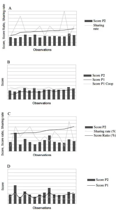
During stage 2 we observe that on average, the score of participants were 28 whereas it was 22 during stage 1. Besides, the score of participants of group B were on average 31 so that the relative performance ratio is on average 41%. The piece rate is on average 51% (c.f. Table 1). That would mean that, participants of group A, when they receive half of the global income but when participants of group B have better performance than them, they increase their effort. Besides we observe that the behavior seems not to depend on the piece rate. Indeed the piece rate has a lot of standard error whereas the variable Score P2 doesn’t. Finally, we observe that the variable Score P2 seems to be related to the variable Score P1 and Score P1 Coop (c.f. Figure 4.1). It means that the participant of group 1 seems to take into account the score of participants of group B during stage 1. Let’s focus now on the case when the relative performance ratio is such that partic-ipants of group A have a better performance then particpartic-ipants of group B during stage 1. During stage 2 we observe that on average the score is 30, whereas it was 25 during stage 1. The relative performance ratio is on average 58%. The piece rate is on average 45% (c.f. Table 2). It would mean that paradoxically, when participants of group B has a lower score during part 1 than participants of group A, and the piece rate is inferior to

50%, participants of group A increase their effort. This is not what we expected in view of previous theoretical prediction we made. But, we can explain this phenomena with the variable Score P1. Indeed, in all the case when participants of group A have a better performance than participants of group B, participants of group A has a performance on average of 25. Whereas, when participants of group A have a lower performance than participants of group B, their performance during stage 1 was 22 on average. It means that, participants of group A take in account their own performance during stage 1 more than the relative performance ratio.

4.2

Econometrics model: unobserved heterogeneity and

endo-geneity issues

In spite of the few data we have, we made an econometrical work with. With our prelim-inary data, we made an regression with a panel data model such as:

ei,t= β1(

qA

qP+ qA)i,t+ β2

λi+ β2s+ β3q2A+ ǫi,t (4.1)

Indeed, ei,t is the effort of agent i at the period t. At each period, each agent will

be matched with a different principal and only one time with each principal. So at each period, the agent will have another principal so that ( qA

qP+qA)i,t will change over time

and individuals. Beside, at each period, the agent will have a different piece rate s. λ will be the individual parameter that create unobserved heterogeneity. It is assumed to be constant over time and not correlated with the other variables. β3q2A will capture

the concavity of the ratio qA

qP+qA. The problem is that after the first stage, we need to

match agent with principal such as we have enough data for each observable ratio qA

qP+qA.

Indeed, otherwise while the regression, if all the value of qA

qP+qA are very clothed to each

other, we will not observe any thing. In the following section we will focus on this issue.

4.2.1 Endogeneity

Endogeneity might comes from the piece rate s which will depend on ( qA

qP+qA)i,t . We

expect this because of the the second prediction of our theoretical model. Indeed, theoret-ically a principal with no legitimacy will increase the piece rate to balance that because he is aware of the agent aversion to illegitimacy. He know the agent will decrease his effort if he observe that the principal has no legitimacy. To resolve this issues we created a intermediate stage called stage 2 in the experiment when the piece rate is actually not

Figure 4.1: Result: Score P2. A: Score Ratio and Sharing Rate (Score Ratio < 50%). B: Score P1 and Score P1 Coop (Score Ratio < 50% ). C: Score, Score Ratio, Sharing Rate (Score Ratio >50%). D: Score P1 and Score P1 Coop (Score Ratio >50%)

chosen by the principal but chosen randomly by the computer. Then we are sure that s do not depend on qA

qP+qA.

Another idea to solve the endogeneity issue is to make a baseline treatment when the participant do not observe their respective performance during stage 1. We would then observe the behavior without information about legitimacy and then just observe the direct effect of the piece rate s and maybe some reciprocity behavior. This baseline treatment would allow us to use the data from stage 3.

4.2.2 Unobserved heterogeneity

The unobserved heterogeneity comes from the idiosyncratic characteristic and more specif-ically from the λ which is assumed to be stable in the theoretical model. λ is interpreted as the the maximum tolerance to inequity of each individual. In other word, in our theoreti-cal framework it means λ is the tolerance to inequity when the principal as no legitimacy at all. The principal has no legitimacy at all when qA tends to infinite or when qP tend

to zero. We cannot observe the parameter λ in the laboratory.

4.2.3 Fixed effect and random effect model

We used two different model for the regression: a fixed effect model and a random effect model. The fixed effect model solve the problem of unobserved heterogeneity. The fixed model will take off the effect of all idiosyncratic characteristics. With a fixed effect model we get that the value of the coefficient qA

qP+qA is -11,91 which is coherent with

the theoretical model. However the P value is 0,277. What is also interesting is that coefficient of the piece rate is much smaller. Indeed, it is 1,13. And this coefficient is less statistically significant than qA

qP+qA . Indeed, the P value is 0,814.

The problem of the fixed effect model is that the concavity of qA

qP+qA is not taken into

account. It means that when qa is high, the impact of a variation of qA on effort trough qA

qP+qA is lower. Indeed, to take into account this effect we should make a regression with

the variable q2

A which do not depend on period. That why it disappear with a fixed effect

model.

Using a random effect model allow us to take into account the variable q2

A and the

concavity of qA

qP+qA. We made two random effect model. One without adding personnel

informations and one without personnel informations. Those information were collected during the questionnaire at the end of the session. The personnel information allows us to take into account heterogeneity. Indeed, in a random effect, heterogeneity is canceled

like in a fixed model.

Surprisingly, the P Value of qA

qP+qA is lower when we don’t take into account individuals

characteristics. Indeed, it is 0,221 without individual characteristics and 0,263 when we take into account individual characteristics. It means that the coefficient is more statisti-cally significant when we don’t take into account individual characteristics. In both cases, the coefficient is strongly negative. Indeed, the coefficient is -12,606 without individuals characteristics and -11,91945 when we take into account individual characteristics.

However, we observe that the coefficient of q2

Ais very statically significant in both case

with a P value almost equal to zero. But the impact on performance is very low because the coefficient is equal to 0,00246397 when we don’t add individual characteristics in the regression and equal to 0,0293169 when we do.

The piece rate coefficient, like in a fixed effect model, is still not statically significant with a P Value of 0,924 and 0,812.

Performance Agent Coeff Std.Err P Value

qA

qP+qA -11,91 10,64436 0,277

Piece rate 1,134063 4,759314 0,814 Table 3: Fixed effect

Performance Agent Coeff Std.Err P Value

qA

qP+qA -12,606 10,29699 0,221

Piece rate 0,4247245 4,479325 0,924 q2

A 0,0246397 0,0044431 0,000

Table 4: Random effect without individuals characteristics

Performance Agent Coeff Std.Err P Value

qA qP+qA -11,91945 10,64436 0,263 Piece rate 1,134063 4,759314 0,812 q2_A 0,0293169 0061092 0,000 Age 0,1726364 0,2502832 0,490 Education level 0,5205016 2,332341 0,823 Baccalauréat -3,42944 2,287568 0,134 School 1,616684 2,481582 0,515 Wealth 0,3753724 1,486258 0,801 Table 5: Random effect with individuals characteristics

Conclusion

The research question of work was: does business abilities of the manager can increase efficiency of incentive. Our point was to considered business abilities of the manager as a source of legitimacy that could enhance the tolerance to inequity of the agent. The tolerance to inequity is in reference with the aversion to inequity of Fehr and Smith. Our contribution is to assume that the tolerance to inequity, which is assumed to be idiosyncratic in the Fehr and Smith model, depend actually on a relative performance ratio.

The implicit question is that a merit-based promotion system in a firm could be more efficient but paradoxically not because the promotion could be a reward for the employee that induce a higher effort. Indeed, in our study, that would be because the manager would then be more legitimate and then respected. This respect would increase obedience. We did a sharper analysis and distinguish the behavioral aspect of the rational aspect. Indeed, a rational agent would follow orders of a more competent principal because the competent principal change implicitly the function of production or the cost of the task. But in our work we focus in our analyze on the behavioral aspects and intrinsic motivation.

In the first step of our work, we first made a mathematical model that gave us two main prediction of behavior. The first prediction is that when the performance of the manager is lowers than the performance of the agent, every thing held equal the agent will decrease his effort. The second prediction is that if the performance of the manager is lowers than the performance of the agent, he will have to increase the piece rate he proposes in the contract to limit the negative impact of his illegitimacy on the agent effort.

The 5 main assumptions and limits of our model are that: 1) The cost function and production function are explicit. 2) The agent and principal’s performances are mea-sured through the same task. 3) The agent and principal’s performances are exogenous. 4) There is perfect symmetry of information about relative performances, effort and pref-erences. 5)Agent and principal are risk neutral.

In the second step of our work , we designed and performed an experiment. The experiment was based on 3 stages. The first stage was designed to elicit the exogenous relative performance when every participant perform the same task to get ranked. In the second stage, the participant were divided in two groups. One became agents and the others became principals. In this stage, the piece rate is chosen randomly. This stage is designed to avoid expectable endogeneity and reciprocity. In stage 3, every things were similar to stage 2 except that the piece rate were now chosen by the participant of the group B. The point of this stage was to have an endogenous piece rate and a situation

closer to the hypothesis of the theoretical model. But this result are not exploitable yet because of econometrical endogeneity issue. To solve this we should perform another treatment without elicit to participant there relative performance.

In the econometrical work we only focused on the first prediction of the model. In other words, we only try to identify the impact of illegitimacy of the principal on the agent behavior. The main result on stage 2 showed that the coefficient of aversion to illegitimacy was indeed strongly negative and almost statistically significant. It showed also that the impact of the coefficient of illegitimacy aversion is much higher that impact of the piece rate. It showed finally that the impact of the coefficient of illegitimacy aversion is more statistically significant than the impact of the piece rate. These result goes in the direction of the theoretical model and could inspire us to perform other session.

This research work set the basis of furthers research.

Indeed, the experiment allowed us to work with a panel data of 7 individuals on 4 period and we hope that with more data we could have statistically significant result. Besides, we hope that we could increase the standard error of the performance of par-ticipant during the stage by make this stage longer. So we could observe bigger spreads between agent’s performance and principal’s performance. That could enhance the legit-imacy/illegitimacy effect on behavior.

Indeed, theoretically that would be interesting to take off some assumption from the theoretical model. The first assumption is that the cost function and the production function are explicit so we could try a more general model. The assumption is that the agent and the principal perform the same task. We could assume two task, business task for the agent and management task for the principal, in a production function. That could be a way to insert management ability as a expected source of legitimacy. We could also make a 2 periods model, that would make relative performance endogenous. Finally, we could stop assuming symmetry of information. More specifically, we could assume that the agent has no information on the performance of the principal. He would then interpret incentive strategic behavior as a signal on his competence.

References

[Aghion and Tirole, 1997] Aghion, P. and Tirole, J. (1997). Formal and real authority in organizations. Journal of Political Economy, 105(1):1–29.

[Anderhub and Gachter, 2002] Anderhub, V. and Gachter, S. (2002). Efficient contract-ing and fair play in a simple principal-agent experiment. Experimental Economics.

[Andrew and Burt, 1975] Andrew, H. and Burt, M. R. (1975). Components of "author-ity" as determinants of compliance. Journal of Personality and Social Psychology, 31(4):606–614.

[Arbak and Villeval, 2007] Arbak, E. and Villeval, M. C. (2007). Endogenous leadership selection and influence.

[Englmaier and Wambach, 2010] Englmaier, F. and Wambach, A. (2010). Optimal incen-tive contracts under inequity aversion. Games and Economic Behavior, 69(2):312–328. [Fehr and Schmidt, 2000] Fehr, E. and Schmidt, K. M. (2000). Fairness, incentives, and

contractual choices. European Economic Review, 44(4):1057–1068.

[Gill and Prowse, 2012] Gill, D. and Prowse, V. (2012). A structural analysis of dis-appointment aversion in a real effort competition. The American Economic Review, 102(1):469–503.

[Hermalin, 1998] Hermalin, B. (1998). Toward an economics theorie of leadership: Lead-ing by example. American Economic Review, Vol 88(5).

[Jong and Schalk, 2010] Jong, J. d. and Schalk, R. (2010). Extrinsic motives as modera-tors in the relationship between fairness and work-related outcomes among temporary workers. Journal of Business and Psychology, 25(1):175–189.

[Ku and Salmon, 2013] Ku, H. and Salmon, T. C. (2013). Procedural fairness and the tolerance for income inequality. European Economic Review, 64:111–128.

[Laffont and Martimort, 1998] Laffont, J.-J. and Martimort, D. (1998). Collusion and delegation. The RAND Journal of Economics, 29(2):pp. 280–305.

[Melumad et al., ] Melumad, N., Mookherjee, D., and Reichelstein, S.

[Potters et al., 2005] Potters, J., Sefton, M., and Vesterlund, L. (2005). After you, en-dogenous sequencing in voluntary contribution games. Journal of Public Economics, 89(8):1399 – 1419. The Experimental Approaches to Public Economics.

[Reichmann and Rohlfing-Bastian, 2013] Reichmann, S. and Rohlfing-Bastian, A. (2013). Decentralized task assignment and centralized contracting: On the optimal allocation of authority. Journal of Management Accounting Research, page 131112123526003. [Schnedler and Vadovic, 2011] Schnedler, W. and Vadovic, R. (2011). Legitimacy of

[Thibaut and Walker, 1975] Thibaut, J. W. and Walker, L. (1975). Procedural justice : a psychological analysis / John Thibaut, Laurens Walker. L. Erlbaum Associates ; distributed by the Halsted Press Division of Wiley, Hillsdale, N.J. : New York. Includes indexes. Bibliography: p. 142-145.

[Tyler and Blader, 2003] Tyler, T. R. and Blader, S. L. (2003). The group engagement model: Procedural justice, social identity, and cooperative behavior. Personality and social psychology review, 7(4):349–361.

[Van Wart, 2013] Van Wart, M. (2013). Lessons from leadership theory and the contem-porary challenges of leaders. Public Administration Review, 73(4):553–565.

[Vollan et al., 2013] Vollan, B., Zhou, Y., Landmann, A., Hu, B., and Herrmann-Pillath, C. (2013). Cooperation under Democracy and Authoritarian Norms. Department of Economics (Inst. fÃŒr Wirtschaftstheorie und Wirtschaftsgeschichte).

[Wulf, 2007] Wulf, J. (2007). Authority, risk, and performance incentives: Evidence from division manager positions inside firms. The Journal of Industrial Economics, 55(1):169–196.

Remerciements

Je souhaiterais remercier Stéphane Robin, Marie Claire Villeval, Quentin Thevenet, Nico-las Houy, Nelly Wirth, Rémi Suchon, Julien Bénistant, Charlottes Saucet et Liza Charroin pour leurs aides, leurs conseils et le temps qu’il m’ont accordé.

Appendix

Instructions

Nous vous remercions de participer à cette expérience sur la prise de décisions. Vos gains dépendent de vos décisions et des décisions des autres joueurs. Il est donc important que vous lisiez attentivement les instructions suivantes. A partir de maintenant et jusqu’à la fin de l’expérience, nous vous demandons de ne plus communiquer entre vous. Pendant l’expérience, nous ne parlerons pas d’Euro mais d’UME (Unité Monétaire Expérimentale). Tous vos gains seront calculés en UME. À la fin de l’expérience, le montant total des UME que vous avez gagnées sera converti en Euros au taux de: 50UME=1Euro En plus des gains que vous réaliserez durant l’expérience, vous recevrez une prime de participation de 5 Euros. Le montant de vos pertes sera couvert par votre prime de participation. Vos gains vous seront payés en liquide et en privé à la fin de la session. Les autres

joueurs ne connaîtront pas le montant de vos gains. L’expérience est divisée en trois parties. Une fois chaque partie terminée, vous recevrez les instructions pour la partie suivante. Les décisions prises au cours de l’une des parties de l’expérience pourront avoir une influence sur le déroulement des parties suivantes. Les parties 2 et 3 comporteront plusieurs périodes. A chaque période vous obtiendrez un gain. A la fin de la partie 3, une de ces périodes sera choisie de manière aléatoire pour calculer vos gains des parties 2 et 3. Ainsi votre gain total à la fin de la session sera la somme de vos gains pendant la partie 1 et des gains d’une période choisie de manière aléatoire pour les parties 2 et 3.

Partie 1:

Vous allez effectuer une tâche plusieurs fois de suite, un maximum de fois. La tâche con-siste à placer un curseur avec la souris de l’ordinateur sur la position 50 sur un intervalle allant de 0 à 100 (cf figure 1). Vous serez évalué et rémunéré en proportion du nombre de tâches que vous aurez effectuées avec succès, à savoir placer un curseur exactement au niveau 50. Les curseurs seront placés sur plusieurs pages les unes après les autres. Une fois que toutes les taches d’une page seront exécutées avec succès, une autre page apparaîtra. Ainsi, vous pourrez réaliser un nombre illimité de tâches.

Pour chaque tâche réalisée avec succès, vous recevrez un gain de 10 UME. Une période de 60 secondes vous sera laissée pour vous entraîner. Durant cette période d’entraînement, les tâches réalisées avec succès ne seront pas prises en compte dans vos gains.

Questionnaire de compréhension partie 1:

1) Supposons que vous ayez obtenu un gain de 40 UME pendant la première partie, de 10 UME, 25 UME,30 UME et15 UME pendant les périodes 1 à 4 de la deuxième partie et de 5 UME, 20 UME, 35 UME et 25 UME pendant les périodes 5 à 8 de la troisième partie. Parmi toutes les périodes des deuxième et troisième parties, c’est la période 5 qui est déterminée aléatoirement pour calculer le gain total. Calculez le gain total:

2) Veuillez s’il vous plait cocher si les affirmations suivantes sont vraies ou fausses: • La tâche consiste à déplacer des curseurs.

Partie 2:

Durant la deuxième partie, vous serez divisés de manière aléatoire en deux groupes de joueurs de même taille: le groupe A et le groupe B. La deuxième partie comportera plusieurs périodes. Au début d’une période, chaque joueur du groupe A est associé à un joueur du groupe B. L’appariement entre joueur est changé à chaque période. Au sein de chaque binôme, les joueurs sont informés du nombre de tâches effectuées avec succès par chacun au cours de la première partie de l’expérience.

Instructions pour un joueur appartenant au groupe A:

Si vous êtes désigné pour appartenir au groupe A, vous continuerez à effectuer la tâche des curseurs. Le but étant de déplacer un maximum de curseurs au niveau 50 pendant le temps imparti.

Instructions pour un joueur appartenant au groupe B:

Si vous êtes désigné pour appartenir au groupe B, vous n’effectuez aucune tâche. Vous percevez une partie des gains du joueur du groupe A. Cette répartition se fera selon un taux de partage que ni le joueur du groupe A, ni le joueur du groupe B ne peut choisir. Ce taux sera déterminé aléatoirement. Exemple: Si le taux de partage est de 0.3, alors pour chaque tâche réussit valant 10 UME, le joueur du groupe A recevra 3 UME et le joueur du groupe B recevra 7 UME. Les deux joueurs sont informés du taux de partage au début de la période. Connaissant cette information, le joueur B doit estimer quel est le nombre de tâches qu’effectuera avec succès le joueur A. Cette estimation ne sera pas communiquée au joueur A.

Calcul des gains pour la deuxième partie Les gains sont fonction du nombre de tâches effectuées avec succès et du taux de partage. Exemple :

Supposons que pour une période le joueur A ait effectué 20 tâches avec succès et que le taux de partage soit de 0.6, nous aurons alors les gains suivants. Gain du joueur A : 0,6 x 20 x 10 UME = 120 UME Gain du joueur B : 0,4 x 20 x 10 UME = 80 UME

Questionnaire de compréhension partie 2:

1) Veuillez s’il vous plait cocher si les affirmations suivantes sont vraies ou fausses: • Durant la partie 2, l’affectation des joueurs aux groupes A et B se fait en fonction

• Durant la partie 2, l’affectation des joueurs aux groupes A et B se fait au hasard. • Durant la partie 2, le joueur du groupe A est informé sur le nombre de tâches

réalisées avec succès pendant la première partie par le joueur du groupe B avec qui il est apparié.

• Durant la partie 2, le joueur du groupe B est informé sur le nombre de tâches réalisées avec succès pendant la première partie par le joueur du groupe A avec qui il est apparié.

• Durant la partie 2, les joueurs du groupe A exécutent une tâche et les joueurs du groupe B n’exécutent pas de tâche.

• Durant la partie 2, les joueurs du groupe A peuvent choisir un taux de partage de leurs gains avec un joueur du groupe B.

• Durant chaque période, les joueurs du groupe A jouent toujours avec le même joueur du groupe B.

• Durant la partie 2, les joueurs du groupe A jouent avec un joueur différent du groupe B à chaque période.

2) Supposons que pour une période le joueur du groupe A ait effectué un score de 15 et que le taux de partage soit de 0,2 alors calculez les gains qui seront attribués :

Au joueur du groupe A : ...UME. Au joueur du groupe B : ...UME.

Partie 3:

Durant la troisième partie, vous serez divisés de manière aléatoire en deux groupes de joueurs de même taille: le groupe A et le groupe B. Les joueurs restent dans le même groupe que celui dans lequel ils ont été préalablement assignés en partie 2. La troisième partie comportera plusieurs périodes. Au début d’une période, chaque joueur du groupe A est associé à un joueur du groupe B. L’appariement entre joueur est changé à chaque période. Au sein de chaque binôme, les joueurs sont informés du nombre de tâches effectués avec succès par chacun au cours de la première partie de l’expérience.

Instructions pour un joueur appartenant au groupe A:

Si vous êtes désigné pour appartenir au groupe A, vous continuerez à effectuer la tâche des curseurs. Le but étant de déplacer un maximum de curseur au niveau 50 pendant le temps imparti.

Instructions pour un joueur appartenant au groupe B:

Si vous êtes désigné pour appartenir au groupe B, vous n’effectuez aucune tâche. Vous percevez une partie des gains du joueur du groupe A. Cependant cette fois-ci, ce sera vous qui choisirait le taux de partage des gains avec le joueur du groupe A. Ce taux ne sera donc plus déterminé aléatoirement. Exemple : Si le taux de partage que propose le joueur du groupe B est de 0.4, alors pour chaque tâche réussie vaut 10 UME, le joueur du groupe A recevra 4 UME et le joueur du groupe B recevra 6 UME. Les deux joueurs sont informés du taux de partage au début de la période. Connaissant cette information, le joueur B doit indiquer quel est le nombre attendu de tâches effectuées avec succès par le joueur A. Cette estimation ne sera pas communiquée au joueur A.

Calcul des gains pour la troisième partie: Les gains sont fonction du nombre de tâches effectuées avec succès et du taux de partage. Exemple : Supposons que pour une période le joueur du groupe A ait effectué un score de 20 et que le taux de partage proposé par le joueur du groupe B est de 0,6 alors voici les gains qui seront attribués :

Au joueur du groupe A : 0,6 x 20 x 10 UME= 120 UME. Au joueur du groupe B : 0,4 x 20 x 10 UME= 80 UME.

Questionnaires de compréhension partie 3:

1) Veuillez s’il vous plait cocher si les affirmations suivantes sont vraies ou fausses: • Vrai Faux Durant la partie 3, l’affectation des joueurs aux groupes A et B se fait

en fonction du nombre de tâches qu’ils ont effectuées avec succès pendant la 1ère partie.

• Durant la partie 3, l’affectation des joueurs aux groupes A et B est la même que durant la partie 2.

• Durant la partie 3, le joueur du groupe A est informé sur le nombre de tâches réalisées avec succès pendant la première partie par le joueur du groupe B avec qui il est apparié.

• Durant la partie 3, le joueur du groupe B est informé sur le nombre de tâches réalisées avec succès pendant la première partie par le joueur du groupe A avec qui il est apparié.

• Durant la partie 3, les joueurs du groupe A exécutent une tâche et les joueurs du groupe B n’exécutent pas de tâche.

• Durant la partie 3, les joueurs du groupe A peuvent choisir un taux de partage de leurs gains avec un joueur du groupe B.

• Durant la partie 3, les joueurs du groupe B peuvent choisir un taux de partage de leurs gains avec un joueur du groupe A.

• Durant chaque période, les joueurs du groupe A jouent toujours avec le même joueur du groupe B.

• Durant la partie 3, les joueurs du groupe A jouent avec un joueur différent du groupe B à chaque période.

2) Supposons que pour une période le joueur du groupe A ait effectué un score de 30 et que le taux de partage proposé par le joueur du groupe B est de 0,2 alors calculez les gains qui seront attribués :

Au joueur du groupe A : ...UME. Au joueur du groupe B : ...UME.