Science Arts & Métiers (SAM)
is an open access repository that collects the work of Arts et Métiers Institute of Technology researchers and makes it freely available over the web where possible.
This is an author-deposited version published in: https://sam.ensam.eu
Handle ID: .http://hdl.handle.net/10985/7618
To cite this version :
Koji HIRANO, Rémy FABBRO - Possible explanations for different surface quality in laser cutting with 1 micron and 10 microns beams - Journal of Laser Applications - Vol. 24, n°1, p.012006 (9 pages) - 2012
Possible explanations for different surface quality in laser cutting with
1 m and 10 m beams
Koji Hirano a)
PIMM Laboratory (Arts et Métiers ParisTech-CNRS), 151 Boulevard de l’Hôpital 75013 Paris, France and Nippon Steel Corporation, Marunouchi Park Building, 2-6-1 Marunouchi, Chiyoda Ward, Tokyo 100-8071, Japan
Remy Fabbro
PIMM Laboratory (Arts et Métiers ParisTech-CNRS), 151 Boulevard de l’Hôpital 75013 Paris, France
a)
Electronic mail: hirano.koji@nsc.co.jp
Abstract
In laser cutting of thick steel sheets, quality difference is observed between cut surfaces obtained with 1 m and 10 m laser beams. This paper investigates physical mechanisms for this interesting and important problem of the wavelength dependence. First, striation generation process is described, based on a 3D structure of melt flow on a kerf front, which was revealed for the first time by our recent experimental observations. Two fundamental processes are suggested to explain the difference in the cut surface quality: destabilization of the melt flow in the central part of the kerf front and downward displacement of discrete melt accumulations along the side parts of the front. Then each of the processes is analyzed using a simplified analytical model. The results show that in both processes, different angular dependence of the absorptivity of the laser beam can result in the quality difference. Finally we propose use of radial polarization to improve the quality with the 1 m wavelength.
I. Introduction
Recent progress of high power and high brightness lasers has enabled high throughput and low cost operation in a number of laser material processing applications in industries. Meanwhile, laser cutting of thick-section steel with inert gas, one of the important applications, has so far failed to benefit from this advantage. The problem concerns striations which are created on cut surfaces during laser cutting process. For thickness typically over ~ 4 mm, roughness of cut surfaces obtained with a fiber or disc laser (L~ 1 m) is higher than that
achieved with a conventional CO2 laser (L= 10.6 m). 1-4
For example, Scintilla et al.4 compared laser cutting of steel with disc and CO2 lasers using almost the same laser beam
diameter and gas condition. For thicknesses of 5 mm and 8 mm, cut surface quality obtained with a disc laser was worse than the one obtained with a CO2 laser. Considering that the
operating conditions were nearly the same, it seems reasonable to infer that the quality difference is attributed to the influence of the laser wavelength on the absorption process and more particularly, the Fresnel absorption.
Whereas wavelength dependence of the Fresnel absorption law has been related to difference in achievable thickness, 5 very few investigations have been made on the mechanism of the difference in the cut surface quality. Poprawe and co-workers observed ripple formations on the kerf front with a 1 m beam but not with a 10 m beam,6,7 which they claim is the cause of the quality difference. This correlation between the ripples on the front and the striations on the sides is not so clear; striations appear even in the case of CO2 laser cutting where the ripple
formations were not observed. Petring et al. 8 has proposed another point of view that multi-reflections, which occur within the kerf in laser cutting with a 1 m beam, can destabilize lower part of kerf sides. According to experimental results, however, the degradation of the surface roughness in the case of a 1 m beam starts at 1 ~ 2 mm below the top surface,1-4 where the laser beam absorption from multi-reflected components is not supposed to be important.
Consequently, multi-reflections cannot be the main mechanism.
One of the problems which have hindered a proper understanding of this phenomenon is that, before discussing details of the wavelength effect, we have not understood properly the mechanism of the striation generation process itself. The situation has been changed, however, by direct experimental observations of the process. Yudin and co-workers observed hydrodynamics on kerf sides during laser cutting of Rose’s alloy9 and mild steel10 by visualization through a glass plate. They confirmed that striations are developed by intermittent downward displacement of melt accumulations along kerf sides. In order to clarify the origin of this intermittent generation of melt accumulations, we observed melt flow dynamics from above the kerf front in laser cutting of steel.11 The results indicated an important role of surface tension, which tends to hold melt accumulations at the top of the kerf side counteracting to assist gas force. Another important phenomenon was found in an intermediate velocity range: melt flow in central part of the kerf front is continuous whereas flow in side parts is discontinuous, and it is this unstable side flow that leads to striation generation. This result indicates the importance of distinction between central and side flows when one considers the influence of the melt flow stability on the striation generation.
The object of this paper is to discuss theoretical aspects of the quality difference observed between the two wavelengths in thick section laser cutting of steel. In the following, we first describe striation generation process suggested from our recent experimental observations, and then discuss possible mechanisms of the quality difference.
II. Mechanism of striation generation
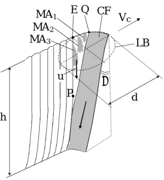
Figure 1 schematically shows melt flow on a kerf front and striation generation process. We pay attention to the three-dimensional structure of the melt flow on the kerf front, considering
the results of our experimental observation,11 which revealed the importance of the distinction of the flows in the central and side parts. This point is contrasted with the existing models (for example, Refs. 6 and 7), where only processes in the central plane of cutting were described.
First of all, it should be noted that, it is the discontinuity of the resolidification process on the kerf side that leads to striations, as was already pointed out by Yudin and Kovalev.9 In the top part of the kerf, the discontinuity comes from discrete melt accumulations (MAs hereafter) that are generated periodically and displaced downwards along the kerf sides. Our observation showed that the MAs are created one by one along an arc EQ in Fig. 1 and displaced downwards almost vertically along the line EP. This line corresponds to the limit of overlapped region of laser beam and the kerf side. As was discussed in Ref. 11, the periodical creation of the MAs is caused by surface tension that tends to retain the MAs at the top surface, and the period of the creation of MAs is determined by force balance between the surface tension and assist gas force.
a
h
V
cd
MA
2CF
E
u
LB
MA
1MA
3Q
P
FIG. 1. Schematic of the striation generation process. (MA: Melt accumulation, CF: Central flow, LB: laser beam)
In lower part of the kerf front, melt flow in the central part can interfere with the side flow as shown in Fig. 1. For example, our observation revealed that in an intermediate velocity region (V = 2 ~ 6 m/min), the MAs, which slide down periodically along the kerf side, are absorbed into continuous central flow11. Below this intersection point, the striations left on the kerf side are mainly determined by the stability of the central flow. The possibility of the interception of MAs by the central flow depends on inclination angle a of the kerf front, downward velocity u of MAs, and so on. When cutting velocity Vc is increased, for instance, a increases and thus the
interception is more likely to occur.
Now let us consider the regime of thick section cutting with a 1 m laser beam, which is the main interest of the present study. In this regime, the central part of the front is expected to be discontinuous, because a is so small. We experimentally investigated the stability of the central part using a 1 m disc laser beam12 and the results showed that, when a < 13 degrees, humps appear in the central part. (Throughout this paper, the term hump is used for a MA that appears in the central part of the kerf front in order to distinguish the one from a MA in the side part, which is called as such.) In general, the maximum value of a can be estimated from (d/h) (h: thickness of specimen, d: laser beam diameter).5 For a typical condition of thick section cutting (h ≥ 4 mm, d ~ 200 m), one obtains a ≲ 3 degrees. The angle is so small that the central part is likely to be unstable. This regime of humps for thick section cutting was reported also in Ref. 6. The humps in the central part can affect striations, since melt flow on the whole kerf front is discontinuous and the humps in the central part can disturb downward movement of MAs on the side through interaction caused by surface tension and can end up in the increase of surface roughness on the kerf sides. This kind of interaction between the central and side flows was observed in our experiments for a low velocity range (V < 2 m/min).11
The above discussion leads us to propose two fundamental processes: the destabilization of the melt flow in the central part, which can disturb the process of downward displacement of MAs and the downward displacement itself, which directly results in striation generation. Each of these two processes is examined in the following. Although there are many parameters that can alter the characteristics of the two processes, we focus on the influences of different wavelengths to clarify the principal mechanism that leads to the quality difference.
III. Stability of melt flow in the central part of the kerf front
First we consider the wavelength dependence of the stability of the melt flow in the central part of the kerf front. The interest of the problem is not limited to the quality problem related to cutting applications. For example, in keyhole laser welding, it is well known that more spatters are generated with a 1 m laser beam than with a 10 m beam. This may be caused by strong metal vapor jet which is emitted from humps on the keyhole front wall.
In spite of its importance, the wavelength dependence of the stability of a cut front or a keyhole front has been scarcely investigated. Koch et al. compared evolutions of keyholes for the two wavelengths with a numerical simulation.13 The keyhole front was found to be stable for a 10 m beam but unstable for a 1 m beam, by changing only the input data of the Fresnel absorption formula. In these simulations, however, constant values of 0.1 and 0.4 were added to the absorption formula for 1 m and 10 m beams, respectively. The validity of this operation is not obvious. Poprawe and co-workers mathematically analyzed the melt film stability.6,7 They found a parameter that measures the degree of the stability. According to the parameter, the system is more stable as
A
sin
sin
becomes small. Here A is the absorptivity, which depends on the local inclination angle a of the front. Using the Fresnel absorption formulae, however, it is easy to show that this derivative term is larger for the 10 m wavelength than for the 1 m in the range of a < 3 degrees, which applies to thick section cutting. It appears that theproposed stability parameter does not correctly represent the wavelength dependence experimentally observed.
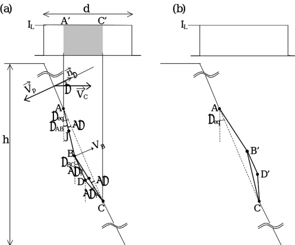
In the present study, the stability of the kerf front is investigated with a simple analytical model, which was used in the past for investigations of keyhole front profiles during laser welding.14-17 We analyze the kerf front in the central plane of cutting, which is shown in Fig. 2(a). The front is represented by a set of chains and the dynamics of the front profile is
A
B
C
D
A’
C’
a
eqa
BCa
a
a
a
h
d
(a)
(b)
I
LI
LV
CV
pn
aV
Ba
A
B’
C
D’
a
eqJ
a
ABA
B
C
D
A’
C’
a
eqa
BCa
a
a
a
h
d
(a)
(b)
I
LI
LV
CV
pn
aV
Ba
A
B’
C
D’
a
eqJ
a
ABFIG. 2. The 2D model of kerf front profiles. Evolution of the profile depends on the sign of the stability function S(a) (see Eq.(7)), where a is the local inclination angle of the front. (a) When S(a) > 0, a concave mode can develop: the node B moves to the left from the line AC, and then the node D to the left from the line BC. (b) When S(a) < 0, an inversed convex mode develops as from the line AC to AB’C and then to AB’D’C.
expressed by displacement of nodes that connect the chains. In the frame attached to the laser beam, displacement velocity of a chain is written as
p c chain V V
V . (1)
Here
V
c is the cutting speed and Vpis the local processing velocity that is expressed by
kI A
nVp L sin , (2)
where n is the normal unit vector of the chain (The subscript adenotes the inclination angle
of the chain.), IL is the laser beam intensity and k is a linear constant, 16,17
which is determined from the energy balance. In fact, if we assume that the surface temperature of the kerf front is equal to the melting temperature Tm, it is easily shown from an energy balance equation that k
-1
≈ Cp(Tm-T0) + Lm within the present 2D approximation (: density, Cp: heat capacity, T0:
ambient temperature, Lm: latent heat of melting). Using Eqs. (1) and (2), the velocity Vchain,
which is defined as the component of
V
chain normal to the chain, is calculated as
V
kI
F
n
V
V
chain
chain
ccos
L , (3)where the function F is defined as
A
sin
F
, (4) for the ease of formulation. By setting Vchain = 0, the angle aeq in the stationary condition isdetermined:
L c eq eqkI
V
A
tan
. (5)Please note that this is a general equilibrium equation for a moving surface subjected to various combinations of IL and Vc. For example, this equation can also be applied to a keyhole front
wall during welding process16,17 with slight modification of the coefficient k. Since A(a)tana increases monotonously with a, aeq is uniquely determined from Eq. (5) for a given
combination of IL and Vc. For simplicity, we assume that the laser intensity is constant at IL, and
Vc. As far as the maximum value of aeq is concerned, it can be estimated independently from Eq.
(5), geometrically by (d/h), which is typically smaller than 3 degrees for thick section cutting. The following discussion assumes a constant value of aeq (< 3 degrees).
Now let us discuss the stability of the kerf front profile. As shown in Fig. 2(a), we consider a small perturbation that displaces the node B to the left (= to the opposite direction of
n
eq ) fromthe straight line corresponding to aeq. The two chains AB and BC, which are assumed to have
the same length, are tilted by (aeq - a) and (aeq + a), respectively. The velocity component of
the node B perpendicular to the straight line AC can be evaluated from the average of the velocities of the two chains AB and BC, which are calculated in the same way as Eqs. (1) and (2):
c eq L
eq
L eq eq L eq c eq L c eq L c BF
kI
V
F
F
kI
F
F
kI
V
n
n
F
kI
V
n
n
F
kI
V
V
eq eq eq eq eq
cos
2
cos
cos
2
cos
2
1
2 2 2 . (6)In order to obtain the final expression, we have neglected terms of the forth order of (a)4 and higher. According to Eqs. (3)-(5), the second term in the right hand side of Eq. (6) is zero. Defining another function S:
F
F
S
2 2 , (7) one obtains
2 2
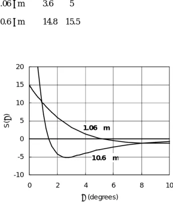
eq L B S kI V . (8)As will be shown in the following, S(ais the key parameter that governs destabilization and it determines a type of unstable modes that can appear. This “stability” function S(a) is shown in Fig. 3 for the two wavelengths of 1.06 m and 10.6 m. For this calculation, the complex refractive indices of iron at T = Tm were taken from Ref. 18 and these values are shown in Table
1. The random polarization was assumed in the calculation. The stability function S(a) takes a positive value at a= 0. It decreases with a and passes zero at some angle. We call this angle a0
that satisfies S(a) = 0. a0 is 1.4 degrees for 10.6 m and 5.2 degrees for 1.06 m. For aa0,
S(a) stays negative for both wavelengths.
Table 1 The complex refractive indices (n + ik) used in the calculation of the stability function S(a)18
Wavelength n k 1.06 m 3.6 5 10.6 m 14.8 15.5
(a) The case of S
eq 0First let us consider the case where S
eq 0 (aeqa0). The equation (8) shows that0
B
V
in this case. Therefore, once the node B is displaced to the left, it gains velocity to the-10 -5 0 5 10 15 20 0 2 4 6 8 10 a (degrees) S ( a ) 10.6 m 1.06 m
FIG. 3. The angular dependences of the stability function S(a) (defined by Eq. (7)) for the two wavelengths of 1.06 m and 10.6 m.
left. Thus the perturbation is amplified. The relation
V
B
0
applies also to the case where the node B is moved to the right, which corresponds to the case of a < 0 for Fig. 2(a). The relation0
B
V
means that the node B is pulled back to the equilibrium position on the straight line AC. In this case (a < 0), the perturbation is suppressed.When the node B is displaced to the left, the perturbation can be amplified more and more. To see this point, let us continue the same discussion as above for the two sets of sub-chains BD-DC, and AJ-JB. First, we consider the case where D and J are both on the straight segments BC and AB, respectively. The velocity component VD0 of the node D normal to the segment BC is
written as
BC
L BC c DV
kI
F
V
0
cos
. (9) Since
BC
eq , one obtainsV
D0
0
from the relation
Vc kIL
A
eq tan
eq A
BC
tan
BC. The velocity component VJ0 of the node J alongAB
n at the same moment is found to be positive, since
AB
eq. This difference of the signbetween VD0 and VJ0 represents initiation of downward transport of the perturbation of ABC
Now let us consider a small perturbation of a1 added to the segment BC. Then the velocity
component VD normal to the segment BC is modified as
0 2 1 1 12
2
1
1 1 D BC L BC L c BC L c DV
S
kI
n
n
F
kI
V
n
n
F
kI
V
V
BC BC BC BC
. (10)We obtain the relation
V
D
V
D0
0
. Therefore, once the point D is displaced by a small amount of distance to the left from the straight segment BC, the point can travel to the left faster than VD0. This makes the section BDC more bended with the segment DC more inclined.Therefore, the initial small perturbation of ABC, can be amplified while transported downwards. There appears a region like DC, where the local a becomes higher and higher. This process of
bending continues as far as S(a> 0, until the local angle a reaches a0 (S(a0) = 0). After this
moment, there will only be the downward transport of the perturbation without further amplification.
(b) The case of S
eq 0Next we consider the case of S
eq 0 (aeqa0). The same discussion as above leads us toconclude that the perturbation to the right as AB’C in Fig. 2(b) increases, since the velocity component VB’ of the point B’ along neqis positive. The segment B’C tends to be bended
further as B’D’C in Fig. 2 (b). The local inclination angle aof the segment D'C becomes smaller than aeqThe growth of the perturbation thus decreases the local aand it stops when
areachesa.
In summary, the above discussion shows that, whatever the initial equilibrium inclination angle aeq is, the kerf profile is inherently unstable (except the case where aeq is exactly equal to
a0). When aeqa0, S
eq 0 and the concave mode as in Fig. 2(a) develops with the increaseof a. On the other hand, when aeqa0, S
eq 0 and the convex mode is amplified with thedecrease of a (Fig. 2(b)). For both cases, the development of the perturbation is terminated when the local abecomes equal to a0. It might be surprising that the kerf front is only stable
when local a is exactly equal to a0. It seems that this result is caused partly by simplifications
used in this model. For example, consideration of surface tension will add a damping effect against the perturbations and should enlarge a stable region of a around a0.
In spite of the simplified assumptions, our model allows us to discuss the interesting point of the wavelength dependence of the stability of the kerf profile as follows. We focus on the low aeq condition for thick section cutting (typically when aeq < 3 degrees).
(i) The case of 10 m
In the case of 10.6 m, S(a) changes its sign at a1.4 degrees. According to the above
discussion, when aeq < 1.4 degrees, S(a) > 0, so the concave mode develops. There appears a
region where a > aeq, but the increase of the local a stops at a1.4 degrees. When 1.4 < aeq <
3 degrees, on the other hand, S(a) < 0. The convex mode appears in this case and the development ceases if the local a is decreased to the same value of 1.4 degrees. In any case, the difference of the angle between a and aeq is small, and thus the corresponding perturbation
along the kerf front is small and cannot grow so large.
(ii) The case of 1 m
For 1.06 m, S(a) becomes zero at a5.2 degrees and is always positive for aeq < 3
degrees. The concave mode appears and this continues to develop until the local areaches a.
Because of the larger value of a, the profile is perturbed much more strongly than the case of
10.6 m. This is considered to be the fundamental reason why the front profile in the case of the 1 m wavelength tends to be less stable than 10 m. It can be added here that a is about the
half of the Brewster angle for each wavelength, so the stability is closely related to wavelength dependence of the Brewster angle.
Although the present model predicts that the local inclination angle can be stagnated at 5.2 degrees for 1 m, more perturbed profiles with much larger acan be observed experimentally. The proper description of this successive development after 5.2 degrees is left for a future work, but it seems possible that the initial perturbation developed up to 5.2 degrees can trigger larger deformation of the profile. Once a so-called shelf or step, where a is locally very high, comes out, strong drilling occurs on the shelf due to higher absorbed intensity. This localized drilling transports the shelf downwards. In the case of welding, strong metal vapor jet emitted from the shelf can destabilize melt pool dynamics. For the striation generation process in laser cutting,
localized melt on the shelf, which we call a hump, can disturb the dynamics of the downward displacement of MAs along the kerf sides.
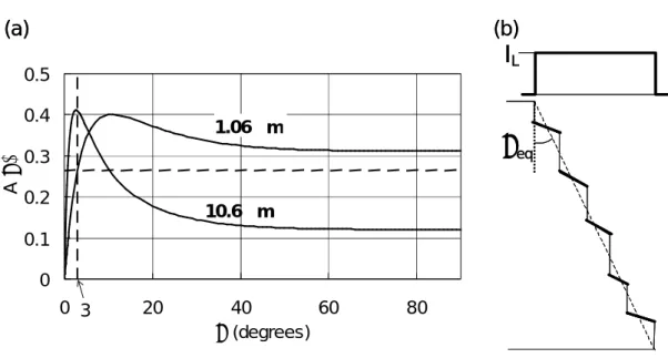
A closer look at the above analysis shows that the perturbation is amplified due to the fact that bending is favorable in terms of energy efficiency. That is, when the straight line AC in Fig. 2(a) is bended, averaged absorptivity for the laser beam section A’C’ increases. It is interesting to note that for 1 m this effect can also be observed in a larger scale, in the energy efficiency of the whole cutting process. Let us consider the absorptivity for a model profile for the hump regime shown in Fig. 4(b). The profile is composed of vertical walls and inclined parts of shelves. The laser beam is then irradiated only on the shelves, where local inclination angle ais much larger than aeq. According to the angular dependence of the absorptivity for 1 m shown
in Fig. 4(a), the absorptivity always increases when ais increased from aeq that is situated in the
range of aeq < 3 degrees. Consequently, when the unstable hump regime is established from the
destabilization effect discussed above in the case of 1 m, the averaged absorptivity can be raised, compared with the case of straight profile with a constant inclination angle aeq. In fact,
0 0.1 0.2 0.3 0.4 0.5 0 20 40 60 80 a (degrees) A ( ) 10.6 m 1.06 m 3
a
eqI
L(a)
(b)
A a 0 0.1 0.2 0.3 0.4 0.5 0 20 40 60 80 a (degrees) A ( ) 10.6 m 1.06 m 3a
eqI
L(a)
(b)
A a FIG. 4. (a) The angular dependences of the absorptivity A(a) for the two wavelengths of 1.06 m and 10.6 m at T = Tm.
18
the increase of the effective absorptivity has already been suggested experimentally: Wandera et al.19 reported that less laser power is required to cut 10 mm thick stainless steel with a fiber laser than with a CO2 laser for the same cutting velocity. Scintilla et al.
4,20
investigated the maximum cutting speed to cut samples of different thicknesses for the two wavelengths, and confirmed that the maximum cutting speed reached by a disc laser is higher than a CO2 laser even for 8
mm thick steel. Also one must note that the averaged values of aeq for these thicknesses (10 mm,
8 mm) are so small that A(aeq) for the averaged angle aeq is higher for CO2 laser (see Fig. 4(a)).
Finally it should be noted that there is another mechanism for the generation of humps. As discussed in Refs. 11 and 21, when aeq is small, humps are generated periodically from the
surface due to combined effect of surface tension and thermal instability. Obviously this mechanism does not depend on the wavelength. Another important difference is that, according to this mechanism, humps are generated only from the surface, whereas humps can emerge anywhere on the kerf front in the case of the destabilization of the front profile discussed above.
IV. Downward displacement of melt accumulations along kerf sides
Let us discuss the influence of the laser beam wavelength on the dynamics of the downward displacement of MAs along kerf sides and on the roughness of striations. As discussed in Ref. 11, the surface roughness is created after the displacement of MAs, which are generated periodically at the top part of the kerf side. The striation wavelength , which corresponds to the width of each of the MAs along the cutting direction, is determined from a balance between force exerted by assist gas and surface tension that retains the accumulations. The downward displacement is almost vertical and the MAs continue to receive laser energy during their downward displacement. Each MA transfers a part of this energy to the solid part. As a result, local melting of the solid part in the contact area creates a stripe of striations.
In thick section cutting, inclination angle of kerf sides is very small, generally less than the angle aeq of the front. For such a small angle, the absorptivity of the laser beam on the MAs
along the sides is higher for 10 m than for 1 m (see Fig. 4(a)). The MAs in the case of CO
laser are thus expected to have higher temperature and consequently lower viscosity. Resultant higher displacement velocity of MAs may reduce the total energy consumed for the local melting during the period of the downward displacement and thus leads to lower surface roughness. This aspect of the temperature dependence of the melt ejection has been pointed out in the past, but the regime of discrete MAs on the kerf side has never been considered. In the following, we examine this rather complex problem with a simplified analytical model and discuss the impact of the temperature of MAs on the final quality of surface roughness.
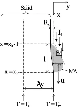
The model that is investigated is shown in Fig. 5. For simplicity we assume that the stationary
T = T
0u
T = T
my
I
Lx
y
l
MA
Solid
R
zx = x
0- l
x = x
0
T = T
0u
T = T
my
I
Lx
y
l
MA
Solid
R
zx = x
0- l
x = x
0
FIG. 5. The 2D model of the striation generation process. The solid part is melted due to heat transfer from the melt accumulation (MA) sliding down along the kerf side wall.
condition is reached. A MA slides down along the kerf side wall with a constant velocity u. It receives laser intensity and transfers a part of the energy to the solid part. As a result, the solid part is eroded by the depth of Rz. The prediction of Rz is the final goal of this analysis. The MA
is assumed to be a deformed droplet, whose characteristic width, thickness and length are given by , and l, respectively. The width corresponds to the striation wavelength, and represents thickness of the MA at the surface, which is also related to the force balance between the surface tension and assist gas. According to our observation,11 it seems reasonable to assume that and are constant. We regard the problem as 2D, reducing the dimension along . The length l of MA increases during the downward displacement, since gradual melting of solid part provides additional volume to MA. Modeling of this complex hydrodynamics is beyond the scope of this work, however, and we assume a constant value of l.
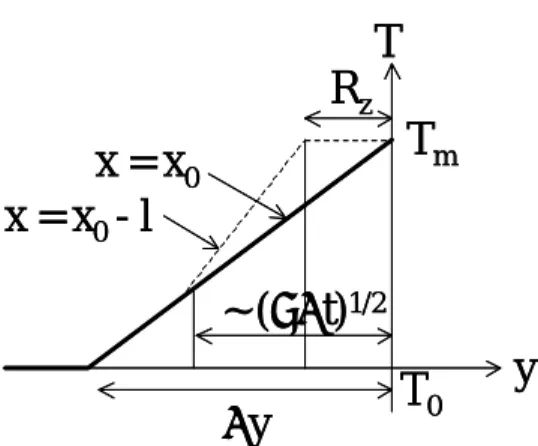
First let us describe the temperature field in the solid part. Before the passage of a MA, the solid part is already pre-heated by heat conduction from the traveling laser beam and the surface temperature reaches Tm, the melting temperature. The initial temperature field inside the solid
has the penetration depth y, which is approximated by y ≈ rk(Pe/2)-0.7 (rk: kerf radius, Pe:
Peclet number(= rkVC/)),11 where the y axis is taken perpendicularly to the solid-liquid
interface. The temperature field is approximated by a linear distribution as the bold line in Fig. 6.
y
T
T
0T
mR
z~ (t)
1/2y
x = x
0- l
x = x
0y
T
T
0T
mR
z~ (t)
1/2y
x = x
0- l
x = x
0Now we examine energy balances around a MA under the condition that the equilibrium is established. The temperature T of the MA is represented by the value at the center of the MA. The first equation comes from the heat flux boundary condition at the surface of the MA:
2
sin
m LT
T
K
A
I
, (11)where IL is the laser intensity, is the inclination angle of the MA’s surface, and K is the heat
conductivity. Please note that the increase of the absorbed intensity in the left hand side results in the temperature increase of the MA. The second equation concerns the Stefan condition along the solid-liquid interface.
w f m
q
v
L
T
T
K
2
, (12)where v is the velocity of the melting front into the solid part, and qw is the heat flux lost into
the solid. Considering that the melting front advances by Rz during the solid-liquid interaction
over the distance l, v can be expressed as
t R
v z
, (13)
where t ≈ (l/u) is the interaction time.
The heat flux qw is determined from the temperature gradient in the solid part. The bold line
in Fig. 6 is the approximate temperature distribution along the line x = x0 shown in Fig. 5, which
corresponds to the moment when the MA arrives. During the interaction time t with the MA, heat flux from the MA penetrates into the solid and the solid-liquid interface moves into the solid part by Rz. Considering that the penetration depth of temperature diffusion can be
approximated with ~(t)1/2, the temperature field after t, along the line x = x0 - l in Fig. 5, can
be approximated as the dotted line in Fig. 6. Please note that the temperature field outside the thickness ~(t)1/2 is not modified in this approximation. One can then calculate the heat flux qw
y T T K l u R y T T K t R dy dT K q m z m z R y w z 0 0 1 1 1 1
. (14)qw is increased by the factor (1-Rz(u/l) 1/2
)-1, compared with the heat flux (≈ K(Tm-T0)/y)
before the arrival of the MA. When the interaction time t is smaller, that is, when the length l of the MA is shorter or the velocity u is larger, qw becomes larger. From Eqs. (12) and (13), one
can see that v and Rz become smaller, which means that the melting is restrained.
Finally we consider kinetics of the MA from a force balance equation. As already mentioned, higher T leads to lower viscosity and higher u. In order to estimate the order of u under the shear stress applied on the surface of MA from assist gas, we refer to a result of an experimental study on droplets sliding down along an inclined surface.22 In this study, a rather general law was found: Ca ~ AmBo, where Am (≈ 0.005 ± 0.002) is a constant, Ca = u/ is the capillary
number and Bo = gsinV2/3/is the Bond number (: surface tension coefficient; inclination angle of the surface; V: volume of the droplet). Replacing the force term (Vgsin) with g(l), which represents the shear force by assist-gas in our case, we obtain
l
A
u
m g . (15)It can be mentioned here that dimensionally Eq. (15) is equivalent to the well-known Newton type viscous friction stress that works on the liquid-solid surface, although in the present case, the droplet slips on the solid surface with the velocity u. The temperature dependence of the viscosity is expressed by the Arrhenius law:
RT
E
aexp
0
, (16)With non-dimensional parameters
L
L
r
k
L
l
,
,
R
z
,u
u
V
C ,
T
T
T
T
0
T
m m
, IIL
Cp
TmT0
VC ,
E
aRT
m, Eqs. (11), (12) and (15) arerewritten as
T Pe A I sin 2 , (17) 7 . 02
1
1
2
Pe
l
u
R
Pe
l
u
R
St
Pe
T
z z
, (18)
k C m g mr
V
A
T
T
l
u
1
exp
, (19) where m a m RT E exp 0
(20)is the viscosity at the melting temperature. The non-dimensional parameter b (Amgrk/mVc) is
about 2.5 ± 1, if we take the values of g 500 Pa, m ≈ 5 x 10 -3
(Pa·s), Vc = 20 (mm/s), rk = 100
(m) and Am ≈ 0.005 ± 0.002. Finally we obtain
T
T
l
b
u
1
exp
. (21)
E
aRT
m
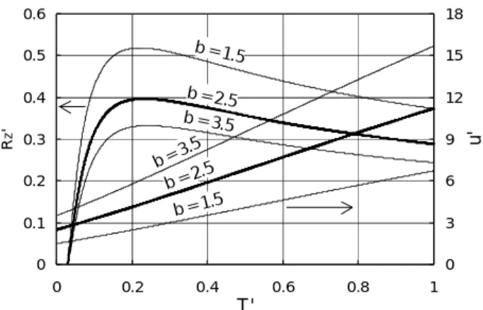
is about 3 for steel.Figure 7 shows the dependencies of Rz’ and u’ on T’ calculated from Eqs. (18) and (21) with
’ = 0.1, l’ = 1.0 and b = 2.5. The curves are shown also for b = 1.5 and 3.5 to see the influence from the variation of Am. It is confirmed that these curves have the same tendency as the case of
b = 2.5, so we discuss only this case in the following. When T’< 0.23 (T < 2.2 x 10³ K), Rz’
increases with the increase of T’. In this temperature region, u’ does not increase strongly with T’, whereas the heat flux through the solid-liquid interface does increases with T’. This
increment of the heat flux is consumed to melt more volume per unit time, which is proportional to (u’Rz’), and thus Rz’ is increased. As u’ and Rz’ increase, however, the heat conduction loss to
the solid part (the second term in the right hand side of Eq. (18)) begins to grow up and the heat flux that can be used to melt the solid is decreased. Consequently Rz’ takes the maximum at T’=
0.23. After this point, Rz’ decreases with T’ mainly due to the reduction of the viscosity with the
increase of T’. For this temperature region, the present simplified model predicts that Rz
decreases with T’, and this can explain the worse quality of cut surfaces obtained with a 1 m beam.
Considering striking difference observed between 1 m and 10 m, however, it seems that the difference predicted by this model is underestimated. Moreover, in reality, the roughness might decrease with the increase of temperature also in the range of T’< 0.23. One way to improve the present model is to take into account the evolution of the geometry of the MA and its effect on the kinetics of the MA. This point will be investigated in a future work.
V. Summary and conclusion
In order to clarify the mechanisms of the quality difference observed in laser cutting of thick section steel with 1 m and 10 m laser beams, we investigated the wavelength dependence of
0 0.1 0.2 0.3 0.4 0.5 0.6 0 0.2 0.4 0.6 0.8 1 T' R z ' 0 3 6 9 12 15 18 u ' b = 1.5 b = 3.5 b = 2.5 b = 3.5 b = 1.5 b = 2.5 0 0.1 0.2 0.3 0.4 0.5 0.6 0 0.2 0.4 0.6 0.8 1 T' R z ' 0 3 6 9 12 15 18 u ' b = 1.5 b = 3.5 b = 2.5 b = 3.5 b = 1.5 b = 2.5
the two fundamental processes.
First we analyzed the destabilization of the melt flow in the central part of the kerf front, which can disturb the dynamics of displacement of MAs (melt accumulations). It is concluded that when the stability function S(aeq) is positive (negative) the concave (convex) mode of
perturbation appears and develops. For both modes, the growth of the perturbations stops when the local inclination angle reaches a0, which satisfies S(a0) = 0. In the case of thick section
cutting (aeq < 3 degrees), the stopping angle a0 for 1 m (5.2 degrees) is far away from the
mean angle aeq of the cutting front, whereas a0 for 10 m (1.4 degrees) is very close to the
operating range of aeq. This explains why the cutting front for a 1 m laser beam is perturbed
much more strongly than that for a 10 m beam.
Then we investigated the dynamics of downward displacement of MAs along kerf sides, which is more directly related to the development of striations. Using a simple analytical model, it was shown that an increase of the absorbed intensity on the MAs can increase their temperature and decrease the surface roughness. This result indicates that the lower absorptivity for very small inclination angle of the kerf sides can be the reason for the worse quality obtained for thick section cutting with a 1 m laser beam.
From these considerations, we finally propose that a possible solution to improve the quality for 1 m is to utilize lasers with the radial polarization. The absorptivity on the kerf side can be increased because the radial polarization works as the favorable p-polarization on the side. To the best of our knowledge, the interest of the use of the radial polarization on the cut surface quality has never been pointed out, while relevant theoretical discussions have focused on improvement of capacity of the cutting process in terms of cut thickness or cutting velocity.23,24 Please note that the cutting capacity is determined mainly by the absorptivity on the central part of the kerf front and not by the absorptivity on the side, which is the present interest.
Experimentally, for CO2 laser cutting of steel, it has already been reported that the surface
roughness can be improved with the use of radial polarization compared to the ordinary circular polarization.25 For the 1 m wavelength, the problem of the destabilization of the central flow may not be completely solved with the radial polarization, because the stoppingangle a0 is still
kept high at 4.8 degrees even for the absorption of the p-polarization. Nevertheless, it is the dynamics of MAs that is directly related to the final surface roughness. Therefore, with the radial polarization, a better absorption of the laser beam on kerf sides should improve the quality to some extent. The authors are willing to see the experimental verifications in near future.
Acknowledgements
The authors would like to thank L. Limat (Paris Diderot University), M.V. Troshin (Tomsk Polytechnic University), P. Yudin (Khristianovich Institute of Theoretical and Applied Mechanics) and K. Sugioka (Tohoku University) for useful discussion and advice.
References
1
C. Wandera, A. Salminen, F. O. Olsen, and V. Kujanpää, “Cutting of stainless steel with fiber and disk laser,” Proceedings of 25th Int. Congress on Applications of Lasers & Electro-Optics (Scottsdale, AZ, 2006), pp. 211-220.
2
T. Himmer, T. Pinder, L. Morgenthal, and E. Beyer, “High brightness lasers in cutting applications,” Proceedings of 26th Int. Congress on Applications of Lasers & Electro–Optics (Orlando, FL, 2007), pp. 87-91.
3
P. A. Hilton, “Cutting Stainless Steel with Disc and CO2 Lasers,” Proceedings of 5th Int.
Congress on Laser Advanced Materials Processing (Kobe, Japan, 2009), Paper 306.
4
L. D. Scintilla, L. Tricarico, A. Mahrle, A. Wetzig, T. Himmer, and E. Beyer, “A comparative study on fusion cutting with disk and CO2 lasers,” Proceedings of 29th Int. Congress on Applications of Lasers & Electro–Optics (Anaheim, CA, 2010), pp. 249-258.
5
A. Mahrle, and E. Beyer, “Theoretical aspects of fibre laser cutting,” J. Phys. D: Appl. Phys. 42, 175507 (2009).
6
R. Poprawe, W. Schulz, and R. Schmitt, “Hydrodynamics of material removal by melt expulsion: Perspectives of laser cutting and drilling,” Physics Procedia 5, 1-18 (2010).
7
G. Vossen, J. Schüttler, and M. Nießen, “Optimization of Partial Differential Equations for Minimizing the Roughness of Laser Cutting Surfaces,” In Recent Advances in Optimization and its Applications in Engineering (M. Diehl et al. (eds.), Springer-Verlag, Berlin/Heidelberg, 2010), pp. 521-530.
8
D. Petring, F. Schneider, N. Wolf, and V. Nazery, “The relevance of brightness for high power laser cutting and welding,” Proc. 27th Int. Congress on Applications of Lasers & Electro–Optics (Temecula, CA, 2008), pp. 95-103.
9
P. Yudin, and O. Kovalev, “Visualization of events inside kerfs during laser cutting of fusible metal,” J. Laser Appl. 21, 39-45 (2009).
10
E. Grigory, P. Yudin, E. Verna, and T. Jouanneau, “Visualization and modeling of combustion effects at laser cutting of mild steel with oxygen,” Proceedings of Pacific Int. Conference on Applications of Lasers & Optics 2010 (Wuhan, China, 2010), Paper 905.
11
K. Hirano, and R. Fabbro, “Experimental investigation of hydrodynamics of melt layer during laser cutting of steel,” J. Phys. D:Appl. Phys. 44, 105502 (2011).
12
K. Hirano, R. Fabbro, “Experimental observation of hydrodynamics of melt layer and striation generation during laser cutting of steel,” Physics Procedia 12, 555-564 (2011).
13
H. Koch, K.-H. Leitz, A. Otto, and M. Schmidt, “Laser deep penetration welding simulation based on a wavelength dependent absorption model,” Physics Procedia 5, 309-315 (2010).
14
A. Matsunawa, and V. Semak, “The simulation of front keyhole wall dynamics during laser welding,” J. Phys. D: Appl. Phys. 30, 798-809 (1997).
15
A. Kaplan, “A model of deep penetration laser welding based on calculation of the keyhole profile,” J. Phys. D: Appl. Phys. 27, 1805-1814 (1994).
16
4075-4083 (2000).
17
R. Fabbro, and K. Chouf, “Dynamical description of keyhole in deep penetration laser welding,” J. Laser Appl. 12, 142-148 (2000).
18
F. Dausinger, and J. Shen, “Energy Coupling Efficiency In Laser Surface Treatment,” ISIJ International 33, 925-933 (1993).
19
C. Wandera, V. Kujanpää, and A. Salminen, “Laser power requirement for cutting thick-section steel and effects of processing parameters on mild steel cut quality,” Proceedings of the Institution of Mechanical Engineers, Part B: Journal of Engineering Manufacture 225, 651-661 (2011).
20
L. D. Scintilla, L. Tricarico, A. Wetzig, A. Mahrle, and E. Beyer, “Primary Losses In Disk And CO2 Laser Beam Inert Gas Fusion Cutting,” Journal of Materials Processing Technology,
accepted for publication (2011).
21
V. S. Golubev, Melt removal mechanisms in gas-assisted laser cutting of materials Eprint No. 3 (ILIT RAS, Shatura, 2004).
22
T. Podgorski, J.-M. Flesselles, and L. Limat, “Corners, Cusps, and Pearls in Running Drops,” Phys. Rev. Lett. 87, 036102 (2001).
23
V. G. Niziev, and A. V. Nesterov, “Influence of beam polarization on laser cutting efficiency,” J. Phys. D: Appl. Phys. 32, 1455-1461 (1999).
24
A. V. Zaitsev, O. B. Kovalev, A. M. Orishich, V. M. and Fomin, “Numerical analysis of the effect of the TEM00 radiation mode polarization on the cut shape in laser cutting of thick metal
sheets,” Quantum Electronics 35, 200-204 (2005).
25
M. A. Ahmed, A. Voß, M. M. Vogel, A. Austerschulte, J. Schulz, V. Metsch, T. Moser, and T. Graf, “Radially polarized high-power lasers,” Proceedings of SPIE 7131, 71311I (2009).