Reliability approach on impacted composite materials for railways

is an open access repository that collects the work of Arts et Métiers Institute of Technology researchers and makes it freely available over the web where possible.

This is an author-deposited version published in: https://sam.ensam.eu Handle ID: .http://hdl.handle.net/10985/8652

To cite this version :

Frédéric DAU, Laurent GUILLAUMAT, Francis COCHETEUX, Thomas CHAUVIN - Reliability approach on impacted composite materials for railways - Revue des Composites et matériaux avancés - Vol. 22, n°1, p.91-114 - 2012

Any correspondence concerning this service should be sent to the repository Administrator : archiveouverte@ensam.eu

materials for railways

Frédéric Dau

1

_{,Laurent Guillaumat}

2

_{, Francis Cocheteux}

3

_,

_Thomas

Chauvin

3

1.Institut de Mécanique et Ingénierie de Bordeaux (I2M)

site Arts et Métiers ParisTech, Centre Etudes et Recherches de Bordeaux-Talence Esplanade des arts et métiers, F-33405 Talence cedex

f.dau@i2m.u-bordeaux1.fr

2.Arts et Métiers ParisTech, Centre d'Etudes et Recherches d'Angers 2 Bd du Ronceray, BP 93525, F-49035 Angers cedex 1

laurent.guillaumat@ensam.eu

3.Agence d'essais ferroviaires

21 av. du président Allende, F-94407 Vitry sur seine cedex

RÉSUMÉ. This paper deals with a reliability approach applied on composite plates which

should be used in railway structures under low velocity impact loading.

Impacted composite plates in bending configuration are considered as an application of the reliability approach to composite materials. Mass of projectile, height of fall and distance between supports are the three variables considered. A limit state function G is defined by the impact force compared to a critical one. Using reliability approach, the reliability index



allows to estimate the probability of failure

P

_f. It is then assessed for several values of the critical force using Monte Carlo direct method and First Order Reliability Method (FORM) approximated method. For FORM method, genetic algorithms are investigated to obtain the best reliability index



. Results obtained by the approximated FORM method are finally discussed and compared to Monte Carlo simulations considered as a reference .

KEYWORDS: impact, damage, reliability, genetic algorithm.

1. Introduction

Fatigue is known to be responsible for the majority of failures of structural components in transportation applications but impact loading is also critical due to damage not always visible (Ballère & al., 2009). The main subject of this research is to develop a reliability approach (Méalier & al., 2010; Lemaire, 2008) for analyzing a composite plate under low velocity impact loading when variabilities are taken into account . Applying such a reliability approach on composite materials is not so usual in literature.

Both experimental and numerical aspects are performed in the present work. Experimental investigations concern the impact tests on composite plates using experimental design technique while numerical ones are related to mechanical reliability models based on experimental results to predict the probability of failure taking into account variabilities. Impact tests have been carried out to understand the main damage mechanisms and to determine the different mechanical responses of the impacted structure: the contact force between the striker and the sample, the contact duration and the out of plane displacement. Previous mechanical responses have been represented using the Response Surface Methodology (RSM) established from the experimental design. Each investigated response is then modeled by an empirical polynomial for which the coefficients are calculated from the chosen experimental design (Doehlert, 1970, 1972). For reliability analysis, the projectile mass (m), the height fall (h) and the span of the simply supported composite plate (p) are considered as mechanical uncertain input variables. The maximum value of the contact force, denoted by Fcontact, is analysed as the mechanical output response variability thanks to reliability tools so that the reliability index

_

and the failure probability level

P

fcould be achieved. Then, direct Monte Carlo method and

approximated First Order Reliability Method (FORM) are especially investigated. The reliability index

_

, needed for numerical FORM application is determined using Genetic Algorithm (GA) (Cantú-Paz, 2000) coupled with Deterministic Algorithm (DA), an original alternative (DA) mainly used in the most of current reliability tools. Results obtained by the approximated FORM method are finally discussed and compared to Monte Carlo reference simulations before concluding.

2. Experimental stage 2.1. Impact device

The impact tests have been performed using a dropping mass set-up designed in our laboratory to simulate accidental falls on a structure, Figure 1. The contact force history between the striker and the composite specimen is measured by a piezoelectric sensor clamped to the mass. A first laser sensor placed just underneath the center of the specimen provides the out-of-plane displacement history. Such a sensor allows measurement without contact. It is particularly adapted to dynamic

measurement. A second laser sensor measures the striker displacement versus time so that the velocity of the dropping mass can easily be assessed.

2.2. Composite samples and striker

The plate used in this study is made of an eight layers carbon/thermoset laminated composite. It was elaborated by hand lay-up technique and was cured under vacuum. Samples were cut from a large plate for which : i) the total thickness is close to 4.2mm and ii) the fiber volume fraction is estimated to 56%.

Each sample is simply supported on two metallic supports fixed on a solid mass and impacted on its center, Figure 1.

The stricker is hemispherical of diameter 16 mm. It is supposed to be indeformable.

Fig. 1. Drop tower and composite sample.

2.3. Impact tests

Three main parameters have been chosen to qualify a test : mass and velocity of the striker and the span. The width of the plate is defined such as the ratio 'width/span' remains a constant value (about 3.00) so that results could be compared more easily. For each test the different values for all the parameters are suggested by an experimental design (Droesbeker, 1997). Doelhert experimental design based on simplex method is adopted (Doehlert, 1970, 1972) due to its main properties: i) the experimental points are uniformly distributed in the experimental design space ii) new variable can be easily added iii) this is a second order design space which permits to elaborate surface response on the mathematical form given in Eq. (1).

height (h)

mass (m)

Y=a0

∑

i=1 n ai. xi

∑

i=1 n aii. xi. xi

∑

i=1 n

∑

ji n aij. xi. xj (1)

Setting up an experimental design method involves several steps. Firstly, the nature and limit values of the variables must be fixed. The degree of the polynomial must then be chosen. Thereafter, the matrix giving all the values for the parameters can be established according to strict rules (Droesbeker, 1997). Moreover, in order to make easier the determination of the relative influence of the different parameters, the variables are expressed in centred, reduced co-ordinates. Their amplitude of variation is therefore standardized into the range [-1,+1]. Codification is detailed in Table 1.

Table 1 : Impact test parameters in physical and centred reduced co-ordinates.

Variable Name Level +1 Level 0 Level -1

mass (kg) x1 3,50 2,75 2

height (m) x2 1,0 0,6 0,2

span (mm) x3 480 305 130

Using Doelhert theory, the experimental matrix is given by Table 2.

Table 2 : Test matrix using Doelhert theory.

N° 1 2 3 4 5 6 7 8 9 10 11 12 13

X1 0 1 -1 0.5 -0.5 0.5 -0.5 0.5 -0.5 0.5 0 -0.5 0

X2 0 0 0 0.87 -0.87 -0.87 0.87 0.29 -0.29 -0.29 0.58 0.29 -_0.58

X3 0 0 0 0 0 0 0 0.82 -0.82 -0.82 -0.82 0.82 0.82

We can notice that only 13 tests are needed to obtain the empirical polynomial including the influence of the coupling between the different variables (Xi). A last interesting point of the Dolhert approach is that all the variables can not have the same number of level. For instance, x1 can take five different values (-5, -1, 0, 1, 5) while x2 can change 7 times (-0.87, -0.58, -0.29, 0, 0.29, 0.58, 0.87). Advantages are: i) to increase the polynomial approximation accuracy according to particular variables, ii) to limit the number of device settings when discrete parameter is involved (the mass for instance).

Then, polynomial coefficients, â, are estimated using a multilinear regression, Eq. (2).

a= xt

x−1_xt

y (2)

with a=a0a1a2a3a12a13a23a11a22a33,  xa matrix for which each row

corresponds to a realization 1 x1 x2 x3 x1x2 x1x3 x2x3 x1 2

x₂2 x₃2_{, and}

The quality of the polynomial (Eq. (1)) has to be checked using the variance analysis (Saporta, 1990). It consists in verifying that the approximated response variation,

Fcontact, is really involved by variation of parameters X₁, X₂ and X₃ and not due to

experimental noise. Moreover, the total error coming from the choice of the experimental design can be established using Eq. (3) before doing any tests.

e= xtx−1 (3)

An example of e considering only the variable X1, X2, is illustrated in Fig. 2. It can be noticed that the accuracy is lower around the corners of the domain.

Fig. 2. Error due to the type of the investigated experimental design.

Although the analysis of the impact test responses is not the main objective of this work, an example of a registered curve Force versus Time is given in Fig. 3. It represents a mechanical response as a superposition of a quasi-static behaviour and a vibratory part which mainly reveals the striker, the plate and metallic supports eigen modes participation. More details about mechanical behaviour of impacted composites are available in literature (Guillaumat, 2000, 2005).

Fcontactwill correspond to the maximum measured value, that is to say 569 N in the

present case.

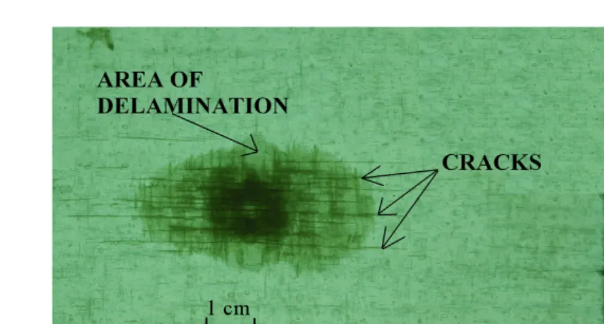
The damage, induced by the impact, is mainly represented by longitudinal localized cracks under the contact zone between the sample and the striker and delamination always inside the cracked zone, Fig. 4.

Fig. 3. Typical force versus time curve.

3. Response modelisation

Based on the previous experimental design, the contact force Fcontactis modeled by a

response surface avoiding heavy calculations with (FE) or numerous experimental tests to assess the variability of the response and perform future reliability analysis. The Fcontactpolynomial estimated by the Eq.2 from the experimental results according to the Doelhert's experimental design (Doehlert, 1970, 1972), is expressed by Eq. (4).

F_contact=1272171 x1485 x2−516 x3−20 x1x271x1x3−79 x2x₃

−97 x12_{−49 x2}2_{262 x3}2 (4)

Using Eq. (4), Fcontactresponse can be then simply evaluated with minimum cost;

only 13 tests are needed to establish this polynomial. A plot of this response is illustrated on Fig. 5 when the mass parameter is fixed to its mean value while the two other ones vary.

Fig. 5. Response surface of the contact force during impact.

According to this plot, the force evolution seems to be physically acceptable; the span decreases (coming from +1 upto -1) the force increases because of the increase of the sample stiffness. Moreover, a slightly nonlinear shape can be noticed for the response surface.

4. Reliability approach 4.1. Performance function

The reliability approach begins by the definition of the physical mechanism responsible of the structure failure. Then, this mechanism is translated into terms of a performance function, denoted G, Eq. (5), which classically compares the stress to the strength of the investigated phenomenon (Lemaire, 1997). In this study, the

maximum contact force

F

_contact(stress) is compared to an ultimate force

F

_ultimate

(strength) such as:

Obviously, the stress and strength can depend on several variables.

G equal to 0 corresponds to the so-called 'limit state function' (Eq. (6)), separating the failure and safety domains as illustrated in Fig. 6.

G

=F

ultimate

−Fcontact=0

(6)

The 'safety domain' (pale area) defined by G>0 and the “failure domain” (dark area) by G<0 are also illustrated in Fig. 6.

Fig. 6. Joint Density of Probability (JDP)

The next step consists in representing the distribution of uncertain quantities. The mass (m), the height (h), and the span (p) are such quantities in this study. They will be described by a normal distribution. This choice doesn't result from any measurements but it is only an assumption coming from the fact that generally physical data is well described by such a distribution.

It is quite obvious that the resulting level of probability can be largely influenced by the nature of the input variable distribution. The proof is given in Fig. 7 where two different statistical distributions (Gaussian and uniform) were used to compare their influences on the probability level. Monte Carlo method (see bellow) was applied on Eq. 6 using Eq. 4 for the

F

contact_{to obtain these probabilities.}

Fig. 7. Statistical distributions influence on probability levels

A great variation between the two situations can be noted. The Gaussian law provides a lower probability level because the values are more concentrated around the mean compared to the uniform law. Thus, the frequency of a value far from the mean is lower in a Gaussian case that implies a lower probability level. This simple example highlights the large influence of the distribution choice which has been established using mechanical tests.

4.2. Failure probability assessment

Classically, several methods are available to perform reliability analysis following the main objective: to estimate the failure probability or a reliability index. To this purpose, the following methods are often used: Monte-Carlo, the derivative Monte Carlo method such as Monte Carlo by importance sampling (Lemaire, 2008), and the others approximated methods such as First Order Reliability Method (FORM) and Second Order Reliability Method (SORM).

In Monte-Carlo approach, all the variables are randomly sampled according to their statistical distribution in order to create a random vector. For each trial (a set of data) the G function; Eq. (5), is then evaluated. The next step consists in counting the number of situations giving G negative. Finally, the failure probability

P

f is

classically estimated by Eq. (7). 

Using this method, it is possible to establish the error depending on the trials number (n) and the estimated probability level: P . It can advantageously be obtained by Shooman (Shooman, 1968) formula, Eq. (8).

% error=200



1− Pf n Pf

(8) On the opposite, this method can be very time consuming when limit state function calculation is complex and needs for instance the use of Finite Element Method (FEM).

From this point of view, the use of a surface response like an empirical polynomial to represent the approximation response Fcontact (see section 3) is quite justified. Then, Monte Carlo approach can be easily performed in this work with minimum cost. Results issued from this 'direct method' will be considered later as reference. On the other hand, the FORM (and SORM) method consists in an analytical

approximation of the failure probability by calculating a reliability index

_

(Hasofer

& Lind, 1974). It is necessary, in this case, to formulate the limit state, Eq. (6), in a reduced variable space, usually called standard space, where each variable distribution becomes a so-called normalized reduced Gaussian distribution after isoprobabilistic transformation. In this standard space, the mean becomes zero, the standard deviation becomes unit, Xi become ui, G becomes H and all the level curves are circular, Fig. 8.

Fig. 8. Isoprobabilistic transformation.

In the case where the statistical distribution in the physical space is a Gaussian, the transformation is simply given by Eq. (9).

ui=xi−mi

i (9)

mi and si stand for mean and standard deviation of xi.

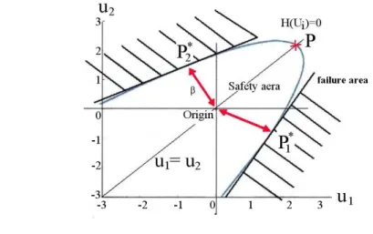
In the standard space, the reliability index

_

represents the shortest distance from

the limit state surface (defined by H) to the origin. Optimization algorithms are then needed to determine this index. Deterministic ones are not always the most efficient to find the global minimum depending on the function to minimize. Thus, genetic algorithms are investigated in this work (see section 4.3) looking for the best value of this index (global minimum) (Cantú-Paz, 2000).

Then, having

_

index, the failure probability can be easily deduced by Eq. (10).

P_{f=−=1− with} = 1



2

∫

−∞  e −u2 2 _du (10)

where

_

stands for the standard normal Cumulative Distribution Function (CDF).

The main assumption in this First Order Reliability Method (FORM) is to consider the limit state as a hyperplane. With FORM method, no error estimation is available contrary to Monte Carlo approach but it is less time consuming.

In general way, coupling several methods for 'reliable' failure probability estimation is preferable in order to obtain the maximum information.

4.3. Obtaining the reliability index

_

The failure probability estimation will be as much suitable than

_

index (needed by

FORM approach) issued from optimization algorithms is sufficiently accurate: its determination is of first importance. In the standard space, the optimization problem is formulated as:

=





∑

_iui

2_{ (11)}

Finding ui which minimize the distance



from the limit state surface to the origin,

Fig. 9, and satisfying:

Hui=0 (12)

Function H in Eq. (12) represents the performance function expressed (Eq. (6)) in the standard space. Moreover, by use of optimization algorithms, Xi variables

corresponding to

_

index can be obtained, which is of prime importance for design.

Having these coordinates, the statistical influence of every variable on the failure probability level can be estimated.

Let's keep in mind that if we consider only R=Fultimateand S= Fcontactas two

Eq. (13). It corresponds to the analytical definition of the smallest distance between the origin and a straight line representing, here, the limit state function.

= R−S



R

2_

S

2 (13)

where R and S respectively denote R and S mean whereas sR and sS denote R and S

standard deviation.

In this work, the

_

index is obtained by various ways: either analytically using Eq.

(13) with R=Fultimate and S= Fcontact variables considered in this case as independent Gaussian variables, (see section 4.2), or numerically using optimization algorithms. Genetic Algorithms (GA) are especially investigated in this study. In this case, x1 (mass), x2 (height) and x3 (span) are also considered as independent Gaussian variables. It is only an assumption in this work but generally they could be represented by any statistical distribution.

Genetic algorithms (GA) (Cantú-Paz, 2000; Chang, 2006; Cheng, 2007; Deep & Tackur, 2007; He & Sýkora, 2007) are here coupled with deterministic algorithms

(DA) to improve global minimum research: the best

_

value is expected in our case.

Generally known to be time consuming when they are coupled to finite element analysis, GA become powerful when the formulation is quite explicit like in this study and when the limit surface has a complicated shape. GA can reveal themselves more efficient than using only DA, even for simple function. Such a case is illustrated Fig. 9 (Méalier & al., 2009) where a paraboloid function is considered. Critical points P1* or P2* (feasible exact solutions) are systematically found with GA whereas point P is often obtained using DA; DA are influenced by gradient descent method and does not converge to the right optimum in this case!

Fig. 9. Paraboloid state limit function.

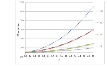
As a consequence, the estimated failure probability could be very different to the right value because of its high sensitivity to this index (see Equ 10). Fig. 10 gives a

good illustration of this phenomenon. Curves indicate the resulting inaccuracy on

the failure probability due to 1%, 2%, 5% and 10% inaccuracy on

_

index.

Fig. 10. Influence of

_

inaccuracy.

Several strategies of research have been investigated for this work to find the better



index. Optimization algorithm GA alone and GA coupled with DA are especially

investigated. Based on GA optimization toolbox program in Matlab software (Matlab software), a new program involving 'Islands' strategy GA algorithm (Maeda & al., 2006) and coupling the previous GA with classical DA (Haftka & Gürdal, 1993) have been developped. This program, named 'GARelDe' (as Genetic Algorithm for Reliable Design) is not detailed in this paper. Many tests have been performed using highly nonlinear and multi-modal limit state function from literature. The good performances of GA coupled with DA, using GARelDe, are proved in the following investigated Test 1 and Test 2. For these tests, illustrations are given in Fig. 11 and Fig. 12, the data are provided in Table 3 and the results in Table 4 and Table 5. For each method, 100 simulations have been performed and a percentage of satisfaction is given. The criterion of satisfaction represents the

number of times leading to the expected

_

index value within a fixed error range.

Table 3

Data for Test1 and Test 2.

Test 1

variables and research range: [x1;x2] in [-5;5]2

performance function: G1 x1,x2=e

design point theorical value: [-2.5397;0.9454] research methods:

- DAMatool: Matlab (Matlab software) Deterministic Algorithm - GAMatool: Matlab (Matlab software) Genetic Algorithm

- GARelDe without coupling: Present tool without coupling GA and DA - GARelDe with coupling: Present tool with coupling GA and DA population for GA application: 90 individuals

Test 2 variables and research range: [x1;x2] in [-10;10]2

performance function:

G2 x1,x2=−100∑ilog

∣

xi−4

∣

50

∣

xi

∣

cos²π /3 xi2 xi−1² design point theorical value: [0.989;0.989] research methods:

- DAMatool: Matlab (Matlab software) Deterministic Algorithm - GAMatool: Matlab (Matlab software) Genetic Algorithm

- GARelDe without coupling: Present tool without coupling GA and DA - GARelDe with coupling: Present tool with coupling GA and DA population for GA application: 90 individuals

Table 4

Comparisons of optimization techniques for Test 1.

Error on

_

±5 % ±10 %

Satisfaction rate in %

DAMatool 100 100

GAMatool 5 8

GARelDe (without coupling) 39 48

GARelDe (with coupling) 100 100

Error on

_

±2 %

Satisfaction rate in %

DAMatool 14

GAMatool 54

GARelDe (without coupling) 27

GARelDe (with coupling) 97

For the simple limit state function used in Test 1, DAMatool and GARelDe lead to the same performances. Neverthless, DAMatool remains the most efficient owing to less consuming time compared to GARelDe with coupling in this case. For the Test 2, GARelDe with coupling is the most efficient algorithm.

Finally, a synthesis of results obtained for all tests is given in Table 6. Design point coordinates are also mentioned in this table.

Table 5

Synthesis for all tests.The results obtained by the present GARelDe program are compared to Theory, Phimeca (Phimeca software), Elegbede (Elegbede, 2005), Gayton (Gayton & Bourinet, 2003), Borri ( Borri & Speranziniones, 1997) and Kiureghian (Kiureghian, 2006) ones.

Performance function Method x1 x2 

 x1−1² x2−1 ² Theory GARelDe 11 11 1.4141.414 e0.2 x11.4−x 2 Theory GARelDe Phimeca Elegbede Gayton -1.680 -1.682 -1.675 -1.688 -1.686 2.898 2.897 2.901 2.893 2.892 3.350 3.350 3.350 3.349 3.348 −1/ 2x1²x2²−2 x1x2− x1 x2/√ 23 Theory GARelDe Phimeca Borri -0.765 -0.744 2.121 -0.752 1.472 1.482 2.121 1.480 1.658 1.659 3.000 1.660 5−1/ 2 x1−0.1 ²−x2 Theory GARelDe Phimeca Elegbede Kiureghian -2.741 -2.741 -2.741 -2.742 -2.741 0.965 0.965 0.966 0.963 0.965 2.906 2.906 2.906 2.906 2.906 e0.4 x126.2−e0.3x25−200 Theory GARelDe Phimeca Elegbede -2.540 -2.540 -2.540 -2.548 0.945 0.940 0.944 0.924 2.710 2.710 2.710 2.710 x1 3 2 x2−5. x1−1² Theory GARelDe 0.617 0.617 0.248 0.251 0.666 0.666 x₂2 −x12 2 −5 Theory GARelDe -1.000-1.001 2.4502.449 2.6462.646 These results confirm the good performance of the association GA (islands strategy , Maeda & al., 2006) and DA in GARelDe computer program. For previous reasons, GARelDe will be used for present application of impacted composite plate.

5. Simulations and results

All variables distributions are supposed, in this study, to be Gaussian, so completely defined by the mean and the standard deviation.

Fultimateis considered as a variable for this work. Its variation is justified by the

Fcontact mean value of 1271 N, which is a constant value in Eq. (1). Fultimateis

considered as a Gaussian distribution, the mean value varies from 600 N to 2100 N by increment of 30 N and the same variance coefficient of 5% is used for each case. In this way, the probability of failure varies from 1 up to a very small value. For each variable x1, x2 and x3, varying in the range [-1,+1] as suggested by the

experimental design (see section 2.3), a zero mean value and 0.2 standard deviation are retained. Choosing a small standard deviation avoids to truncate the distribution. For Monte Carlo approach, the performance function G is directly evaluated by the approximation given in Eq. (4) for Fcontact. A first series of Monte Carlo simulations, denoted MC1, is performed. It consists in one million of trials for each variable. For each variable set, function G is evaluated using Eq. (6). The failure probability is finally estimated by Eq. (7). A second series of Monte Carlo simulations, MC2, is next performed. For this one, only linear terms in Eq. (4) are considered to evaluate

Fcontact and then G function.

Two ways of calculating the

_

index are performed for each Monte Carlo calculation: i) an analytical calculation issued from Eq. (13) where Fultimateand

Fcontact are considered as independent Gaussian variables, as explained in section

4.3. Results are denoted FORM1-Anal when complete expression given in Eq. (4) is used and FORM2-Anal when only first order terms are conserved. ii) a numerical calculationusing genetic algorithms where x1 (mass), x2 (height) and (span) x3 are considered as independent Gaussian variables. Results are denoted FORM1-GA when complete expression given in Eq. (4) is used and FORM2-GA when only first order terms are conserved.

First of all, a comparison between the Monte-Carlo (MC1) and FORM (FORM1-Anal) methods is shown on Figure 13. The Fultimatemean value, used for the Gaussian distribution with a variance coefficient of 5%, is mentioned on the curve in X-coordinate.

Fig. 13. Probability versus Fultimate estimated by MC1 and FORM1-Anal

A gap between the two simulations is obviously visible beyond Fultimate=1500 N.

The main explanations are due to the fact that i) firstly, the number of trial becomes insufficient as regard to the probability level for the Monte-Carlo technique, ii) secondly, second order polynomial (Eq. (4)) induces a non-Gaussian distribution for

Fcontact(Figure 14). So, an error can be observed in the FORM analytical

calculation.

Fig. 14. Fcontact non-Gaussian distribution

Even if the distribution seems to be not so far from a Gaussian distribution, it has not strictly the right shape. It means that the only knowledge of the mean and the

standard deviation calculated from this distribution are not enough for its complete characterization. Consequently, the FORM method is not powerful in this case. The Henry test (Droesbeker, 1997) also reveals that the Fcontactdistribution is not a Gaussian one (Figure 15) because the obtained points (circle) do not follow a straight line.

Fig. 15. Henry test for a non-Gaussian distribution.

Indeed, this curve obtained by Henry test deviates from the straight line beyond Fcontact~1500 N, that means that Fcontactdistribution deviates from a Gaussian distribution from this value.

Percentage of error obtained with Monte Carlo method, coming from Eq. (8), is mentioned for different values of Fultimate, see Figure 8. It indicates that Monte Carlo results are probably reliable until Fultimate~1900 N ; approximatively 10% error is reached at this level. Beyond this value, % error rapidly increases. The number of simulations becomes insufficient.

On the other hand, results issued from MC2 and FORM2-Anal (only linear terms are kept for Fcontact) are compared on Fig. 16.

Fig. 16. Probability evolution evaluated by MC2 and FORM2-Anal.

Figure 17 shows the result of the Henry test applied on the distribution representing the polynomial with only the linear terms. The distribution can be now considered as a Gaussian one.

Fig. 17. Henry test for a Gaussian distribution.

Better agreement is observed compared to the previous case (Figure 13). FORM approximated method gives an 'exact' estimation of the failure probability due to the Gaussian nature of all the distributions used in this simulation. Concerning Monte Carlo results, same remarks than previous ones for MC1 can be done. Results are reliable as much as the number of simulations is in agreement with the expected probability level. The limit of result validity is around Fultimate~1850 N. Beyond this

value, error is over 10% and rapidly increases. On the opposite, FORM2-Anal gives correct failure probability estimation without limitation. Indeed, as FORM2-Anal results are validated by MC2 ones for high probability levels (till around Pf=3.10-4 corresponding to 10% error), the validation can be extended for small probabilities level as regards FORM properties in this case of linear limit state function.

Moreover, MC1, FORM1-Anal and FORM1-GA results are finally presented on Figure 18. Those obtained by FORM1-GA are encouraging but need to be improved as regards discrepancies for low probability levels. Obviously, this technique should be better in case of complex shapes for the limit state function.

Fig. 18. Comparison between FORM1-Anal, FORM1-GA and MC1.

Finally, this kind of results is very usefull for designers to define some dimensions

of the structure for a given probability of failure. For example, in our case the x3

variable (span) could be considered as a distance between two panel stiffeners. It means that using the methodology developed in this work, it is possible to link some structures data to a level probability in order to estimate a risk.

6. Simulations and results

In this work, a reliability approach for designing composite plates as a part of railway structure under low velocity impact loading is developed. A methodology is presented for this approach. First of all, it consists in using experimental design to approximate correctly the interaction force between the structure and the striker

Fcontact during the impact. Doing so, the limit state function G comparing Fcontactto

calculated by FORM determining the reliability factor

_

either analytically or numerically. Genetic algorithms are principally investigated for the numerical way. Results issued from each technique are compared to Monte Carlo simulations

standing for reference. Good agreement are observed. Feasibility of

_

determination

using genetic algorithms is very satisfying and encouraging. In this case of explicit problem formulation, previous algorithms happen to be interesting. Nevertheless, they may be used carefully and the crossing of several methods is indispensable. Future works are envisaged to consolidate the present approach and to deal with performance functions involving local damage mechanisms in composite such as debonding, delamination, crackings .

Bibliographie

Ballère L., Viot P., Lataillade J.L., Guillaumat L., Cloutet S., Damage tolerance of impacted curved panels, International Journal of Impact Engineering,Vol. 36, Issue 2, February 2009, p. 243-253.

Méalier N., Dau F., Guillaumat L., Arnoux P., Reliability assessment of locking systems, Probabilistic Engineering Mechanics, 2010

Lemaire M. Reliability of structures. Wiley, 2008.

Doehlert DH. Uniform shell designs. Applied Statistics, 1970, Vol. 19(3), p. 231-239. Doehlert DH, Klee VL. Experimental designs through level reduction of the d-dimensional cuboctahedron. Discrete Mathematics, 1972; Vol.2, p.309-334.

Cantú-Paz E., Goldberg D. E. - Efficient parallel genetic algorithms: theory and practice - Computer Methods in Applied Mechanics and Engineering, 2000, Vol. 186, Issues 2-4, p. 211-238.

Droesbeker JJ, Fine J, Saporta G. Experimental designs. French Statistical Association, Technip Ed., 1997.

Saporta G. Probabilities – Data analysis and Statistic. Ed. Technip, 1990. Guillaumat L., Reliability of composite structures - impact loading. Computers and structures, 00359, Vol 76, Issues 1-3, pp163-172, june 2000.

Guillaumat L., Baudou F., Gomes De Azevedo A.M., Lataillade J. L., Contribution of the experimental designs for a probabilistic dimensioning of impacted composites.

International Journal of Impact Engineering, Vol. 31, Issue 6, pp 629-641, july 2005. Lemaire M. Reliability and mechanical design. Reliability engineering and system safety, 1997, Vol. 55(2), p.163-170.

Shooman M.L., Probabilistic Reliability: An Engineering Approach. Mc Graw Hill Book co, New-York, NY, 1968.

Hasofer AM, Lind NC. Exact and invariant second moment code format. Journal of Engineering Mechanics Div., 1974, p.100:111-121.

Chang W. D. An improved real-coded genetic algorithm for parameters estimation of nonlinear systems. Mechanical Systems and Signal Processing, 2006, Vol. 20, Issue 1, p.

236-246.

Cheng J. Hybrid genetic algorithms for structural reliability analysis., Computers & Structures, 2007, Vol. 85, Issues 19-20, p. 1524-1533.

Deep K., Thakur M. A new crossover operator for real coded genetic algorithms - Applied Mathematics and Computation, 2007, Vol. 188, Issue 1, p. 895-911.

He H., Sýkora O. Parallelization of genetic algorithms for the 2-page crossing number problem Journal of Parallel and Distributed Computing, 2007, Vol. 67, Issue 2, p. 219-241. Matlab Software – Optimization Toolbox

Maeda Y, Ishita M, Li Q. Fuzzy adaptative search method for parallel genetic algorithm with island combination. International Journal of Approximate Reasoning, 2006, Vol.41, p. 59-73.

Haftka R. T., Gürdal Z.,Elements of structural optimization, 3rd _{revised and extended}

edition, 1993, Kluwer Academic Publishers. Phimeca software by Phimeca Engineering SA.

Elegbede C. Structural reliability assessment based on particles swarm optimization - Structural Safety, 2005, Vol. 27, p. 171-186.

Gayton N., Bourinet J.M. CQ2RS : a new statistical approach to the response surface method for reliability analysis Structural Safety, 2003, Vol. 25, p. 99-121.

Borri A., Speranzini E. Structural reliability analysis using a deterministic finite element code -Structural Safety, 1997, Vol. 19, Issue 4, p. 361-382.

Kiureghian AD. Structural reliability software at the University of California. Structural Safety, 2006,Vol. 28, p. 44-67.

Annexe A. Symbols list



: Reliability index

P

f : Probability of failure

Fcontact : Contact force between impactor and target

F

ultimate: Ultimate force

G : Performance function 

Pf: Estimated failure probability

_

: Cumulative Distribution Function (CDF). GA : Genetic Algorithm

DA : Deterministic Algorithm

GARelDe : Genetic Algorithm for Reliable Design FORM : First Order Reliability Method

SORM : Second Order Reliability Method MC : Monte Carlo

Annexe B. Figures list

Fig. 1. Drop tower and composite sample... 3

Fig. 2. Error due to the type of the investigated experimental design...5

Fig. 3. Typical force versus time curve...6

Fig. 4. Delamination and matrix cracks after impact...6

Fig. 5. Response surface of the contact force during impact... 7

Fig. 6. Joint Density of Probability (JDP)...8

Fig. 7. Statistical distributions influence on probability levels...9

Fig. 8. Isoprobabilistic transformation...10

Fig. 9. Paraboloid state limit function...12

Fig. 10. Influence of inaccuracy...13

Fig. 11. Graphical representation of G1 limit state function (test1)...14

Fig. 12. Graphical representation of a multi-modal function (test 2)...15

Fig. 13. Probability versus Fultimate estimated by MC1 and FORM1-Anal ...18

Fig. 14. Fcontact non-Gaussian distribution... 18

Fig. 15. Henry test for a non-Gaussian distribution...19

Fig. 16. Probability evolution evaluated by MC2 and FORM2-Anal...20

Fig. 17. Henry test for a Gaussian distribution... 20

Fig. 18. Comparison between FORM1-Anal, FORM1-GA and MC1...21

Annexe C. Tables list

Table 1: Impact test parameters

Table 2: Test matrix using Doelhert theory Table 3: Datas for Test1 and Test 2

Table 4: Comparisons of optimization techniques for Test 1 Table 5: Comparisons of optimization techniques for Test 2 Table 6: Synthesis for all tests