Etude multi-échelle du couplage matériau-procédé pour l'identification et la modélisation des variabilités au sein d'une structure composite

(1)

(2)

(3)

Remerciements

Ces travaux de thèse ont été réalisés à l’Institut Clément Ader et ont été financés par le gouvernement mexicain grâce à une bourse du Consejo Nacional de Ciencia y Tecnología (CONACyT).

Je veux tout d’abord remercier énormément mon directeur de thèse, Francis Collombet, pour toute son aide et encouragement tout au long de cette longue et difficile route qui m’a conduit à la soutenance.

J’adresse également mes remerciements à Bernard Douchin pour ses commentaires toujours critiques et pertinents, et cela toujours dans la bonne humeur quelles que soient les circonstances.

J’adresse aussi un grand merci à Laurent Crouzeix qui a énormément contribué à l’avancée de ces travaux grâce à la vertu créative de ses idées et des discussions toujours d’un très grand intérêt.

Toute ma gratitude va vers les membres du jury qui m’ont fait l’honneur de lire ce manuscrit de façon critique et attentionnée.

Je suis très reconnaissant envers mes rapporteurs, messieurs Alaa Chateauneuf et Jacques Renard, pour le travail et l’attention qu’ils ont bien voulu apporter dans l’analyse de ce travail de thèse. Je suis très honoré qu’ils aient fait montre d’une analyse avec un grand souci du détail aussi bien du point de vue de la forme que du fond.

Ma reconnaissance va aussi vers à monsieur Peter Davies dont les commentaires et la relecture du manuscrit ont été précieux.

Je veux remercier Yves-Henri Grunevald pour ses apports permanents au travers de longues discussions sur ce sujet complexe en y apportant tout son expertise industrielle et sa vision scientifique très avancée dans le domaine des composites.

(4)

J’exprime toute ma reconnaissance à Nathalie Gleizes-Rocher qui m’a, non seulement aidé pour l’analyse expérimentale, mais qui m’a aussi accompagné pour de nombreuses démarches administratives. Je lui serai toujours reconnaissant pour sa bonne humeur et sa gentillesse jamais démenties, chapeau Nathalie !

Je veux remercier également les membres de l’Institut Clément Ader, Philippe Olivier, son directeur, et notamment Jean-Noël Périé et Philippe Marguerès avec qui j’ai eu des discussions animées et intéressantes.

Une thèse n’est pas seulement un exercice solitaire et j’en ai eu la démonstration tout au long de ces dernières années. Je veux remercier tous les stagiaires qui m’ont aidé à avancer dans différentes parties de ce travail de thèse et notamment Jean-Daniel Bodin (2011), Yeison Duran Soache (2012), Marian Gălbău et Claudia Consuela (2012), Eric Hernandez (2013) et d’autres qui me pardonneront d’avoir omis de citer leur nom.

Je remercie aussi l’ensemble des doctorants et des post-doctorants pour l’ambiance si agréable au laboratoire. Mes pensées vont aux anciens Mauricio, Bénédicte, François, Christophe, Luis, Nicolas, Zheng, Linh et José. Pour les futurs docteurs Ambre, Sonia, Matthias et Thibaut, je vous souhaite bon courage pour la suite ! Je n’aurai jamais pu réaliser ce doctorat sans l’aide de ma famille, de mes proches qui ont toujours su me soutenir depuis si loin. Une pensée très forte va à mes parents José Angel et Ma. Luisa, à mes sœurs Tere et Marlene, et aussi au petit Barbarito (Luis Adrian) mon neveu.

Enfin, je veux remercier mes amis, qui ont été ma famille à Toulouse et avec qui j’ai passé de grands moments, Misa, Sara, Germercy, Elena, Dinesh, Arturo, Nestor, Tommaso et Mattia. Thank you guys I love you!

(5)

Résumé des travaux en français

Introduction

Ce travail porte sur l’étude des variabilités au sein de plaques composites carbone/epoxy en M10.1/38%/UD300/CHS avec une stratification quasi-isotrope de 16 plis. Un spectre large de variabilités est adressé, depuis le pli non polymérisé jusqu’à la pièce polymérisée, en passant par la phase de drapage et de polymérisation.

L’objectif de l’ensemble des identifications de variabilités est de permettre d’introduire l’effet de ces variabilités dans des modèles de calcul du comportement de la pièce composite, et d’en évaluer l’influence sur le comportement mécanique.

Chapitre 1 : étude bibliographique

Dans ce chapitre 1, on montre que l’étude des variabilités sur des pièces composites reste un problème ouvert qui peut être abordé de plusieurs manières. En effet, il n’existe pas une méthodologie générale applicable pour chaque étape associée à l’établissement de la solution composite. La définition même de la variabilité reste l’interprétation des chercheurs ou des concepteurs.

Sur l’analyse et la conception des structures composites, il existe une quantité importante de méthodes permettant l’introduction des variabilités dans le calcul des propriétés structurelles. La méthode Monte-Carlo est la plus utilisée pour alimenter ce type d’analyse. Elle sert ainsi comme une sorte de benchmark des autres types de méthodes. Malgré la quantité importante de méthodes dédiées à l’étude des problèmes composites, la prise en compte les variations continues des propriétés au sein d’une pièce composite ou la présence d’un défaut localisé sont

(6)

peu ou pas réalisées. Les propriétés mécaniques sont variables à chaque itération mais en utilisant la même valeur pour tous les éléments finis.

De plus, une grande quantité de méthodes pour l’introduction des variabilités est obtenue à partir d’éprouvettes normalisées. Celles-ci n’ont pas la même stratification que la structure finale et elles ne sont pas fabriquées dans des conditions identiques. Il est bien établi que les propriétés de la structure composite dépendent des matières premières et du procédé de fabrication car les interactions entre la matrice et le renfort ont une nature très complexe. Les variabilités au sein des matériaux composites sont souvent regardées comme des défauts, mais elles sont en réalité le résultat de l’interaction d’un nombre non déterminé de paramètres.

Chapitre 2 : Vers une modélisation de la variabilité répartie sur une structure CFRP

Le chapitre 2 explique le parti pris initial de ce travail. Il s’agit de la volonté d’inclure dans des modèles de calcul des variations locales de géométrie et de propriétés matériaux, tout en retenant comme idée principale que ces variations ne devaient pas être distribuées aléatoirement au sein de la structure composite, mais présenter des lois d’évolution spatiale qui soient en accord avec la réalité du matériau. Cette volonté d’injecter des lois d’évolution spatiale contrôlées constitue le fil conducteur des analyses, identifications et modélisation au cœur de ce travail. De plus, l’objectif affiché n’est pas de recréer à l’identique une unique pièce composite en « injectant » des lois d’évolution figées. Il s’agit de proposer une stratégie de modélisation qui respecte la réalité du matériau tout en contenant des grandeurs déterminées aléatoirement afin d’être capable de mener des études variabilistes. On souhaite ainsi restituer le fait que deux pièces a priori semblables ne se ressemblent pas tout à fait. Ainsi pour chaque paramètre étudié, il est proposé une loi mathématique retranscrivant de façon représentative ces variations, et à laquelle on adjoint une étude probabiliste effectuée sur les paramètres pilotant ces lois.

(7)

Résumé des travaux en français Chapitre 3 : Etude des variabilités sur une structure CFRP polymérisée en autoclave

Dans ce chapitre, la fabrication de plaques composites est décrite ainsi que les mesures de certaines propriétés qui sont prises à chaque étape du processus de fabrication.

Le premier paramètre étudié est, suivant l’ordre chronologique de fabrication de la structure composite, les variations de masse surfacique du pli de préimprégné. Une procédure, inspirée d’approches normatives, est proposée pour obtenir une mesure précise de cette grandeur, notamment via la numérisation de l’échantillon afin d’en déterminer l’étendue sans être influencée par les défauts géométriques des bords de l’échantillon. Une variabilité est identifiée sur cette grandeur avec un coefficient de variation de moins de 2 % au sein de chacun des lots de matériaux étudiés. Une forte variation de la masse surfacique entre deux rouleaux différents est mise en évidence. Cependant, aucune corrélation à ce stade n’a pu être identifiée entre la masse surfacique mesurée et la position de l’échantillon au sein du rouleau de pré-imprégné. De ce fait pour ce paramètre, aucune modélisation mathématique de son évolution spatiale n’a été effectuée.

Une fois les structures composites polymérisées, les plaques ainsi créées ont été caractérisées au moyen d’une machine à mesurer tridimensionnelle. On met en évidence des variations conséquentes d’épaisseurs existant entre des plaques de différents lots de pré-imprégné pour un même matériau et une même stratification. Ces différences ont un lien probable avec le flot de résine se produisant au cours de la polymérisation, lui-même étant directement impacté par le choix et la place des produits d’environnement utilisés. De plus, les mesures démontrent que si l’ensemble des plaques ne possède pas une épaisseur constante, elles présentent une épaisseur maximale en leur centre. Une modélisation mathématique de l’évolution spatiale globale de l’épaisseur de la plaque est proposée comme la somme d’une valeur moyenne et de la valeur d’une sinusoïde de longueur d’onde de l’ordre de la longueur de la plaque avec un déphasage de manière à présenter un maximum au centre de la plaque. L’amplitude des écarts

(8)

d’épaisseur entre le centre et les bords d’une plaque est estimée dans cette étude comme supérieure à la valeur de l’épaisseur d’un pli. Il s’agit donc d’un facteur majeur d’écart des propriétés mécaniques entre une représentation géométriquement parfaite de la pièce et la réalité.

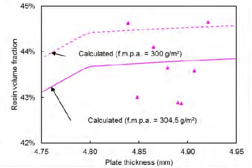
Des analyses physico-chimiques sont réalisées sur des échantillons découpés au sein des plaques ainsi polymérisées. De par la nature de ces analyses, ces mesures n’ont pu être faites qu’à l’échelle de la plaque, et non du pli. L’objectif de ces analyses est de relier l’évolution des propriétés volumiques matériau avec les épaisseurs. Il est montré que le taux de porosité semble augmenter avec l’épaisseur de la plaque, malgré une importante dispersion des résultats. En partant de cette constatation, une loi d’évolution de la porosité en fonction de l’épaisseur est proposée. Cette loi contient un paramètre qui suit une évolution linéaire directement liée à l’épaisseur de la plaque, mais elle est bornée de manière à obtenir une porosité nulle en dessous d’un seuil identifié par les mesures. A ce paramètre dépendant uniquement de l’épaisseur, on ajoute un terme déterminé par un tirage aléatoire basé sur les dispersions identifiées grâce aux mesures expérimentales.

Chapitre 4 : Détermination et modélisation des désalignements de fibres dans le plan apparus pendant le drapage manuel d’un stratifié CFRP

Dans ce chapitre, le paramètre étudié est l’orientation des fibres de chacun des plis. Un système optique est utilisé pour obtenir une image numérique de l’ensemble pli juste après son drapage et avant le drapage du pli suivant. Une analyse des photographies permet de remonter, via l’analyse d’images, aux orientations des mèches de fibres. Ainsi un écart ou une erreur d’orientation moyenne de chaque pli est aisément obtenue. La valeur de cet écart d’orientation semble faible, moins de 2° au maximum, et plus dépendante de l’habilité et de la fatigue de l’opérateur que de la valeur de l’orientation du pli. Une procédure est mise en place pour remonter à un champ d’orientations des mèches au sein du pli. De par la qualité des images et la résolution de l’appareil de mesure comparée à la

(9)

Résumé des travaux en français largeur de la pièce fabriquée, la procédure ne permet pas de remonter à des désorientations sur une zone de petite taille. Malgré cela, la procédure est suffisante pour identifier des évolutions locales d’orientation des mèches de fibres. L’analyse de ces évolutions démontre que toutes les fibres d’un pli ne présentent pas une orientation identique, mais que des zones de plusieurs cm² présentent des écarts par rapport à une valeur moyenne. Ces zones peuvent être par exemple le résultat de la manipulation du pli non polymérisé par l’opérateur. Cependant, on relève que ces zones, dont l’amplitude maximale ne dépasse pas 1°, ne présentent pas de régularité quant à leur position au sein du pli, ni de dépendance suivant l’orientation théorique du pli.

Suite à ces constatations, les lois mathématiques d’évolution de l’orientation à travers un pli proposées contiennent un écart moyen une ondulation systématique dont la valeur est issue de la littérature de travaux anglo-saxons (mais qui n’est pas identifiée dans ces travaux parce que correspondant à des zones trop petites pour être atteignables par la stratégie de mesure), et enfin une somme de perturbations locales correspondant aux écarts identifiés par rapport à la valeur moyenne. Ces perturbations sont modélisées comme des surfaces gaussiennes, et une analyse probabiliste est faite sur l’amplitude et l’étendue de ces surfaces gaussiennes pour en définir des bornes qui soient basées sur la physique du matériau. Il est démontré qu’une somme d’une douzaine de surfaces gaussiennes est suffisante pour représenter fidèlement les évolutions d’orientation au sein de plis de 600 x 300 mm dans le plan. Pour l’exploitation numérique de ces résultats, on fera l’hypothèse que le placement des fibres n’est pas affecté par la polymérisation de la pièce.

Chapitre 5 : Evolution spatiale de la variabilité de l’épaisseur de pli répartie sur une structure CFRP

D’une part, l’étude des variations d’épaisseur des plis dans une section montre que les valeurs pour un même pli peuvent varier, le long de quelques millimètres dans le plan, d’une valeur supérieure à 30 % de sa valeur moyenne.

(10)

D’autre part, les variations d’épaisseur des plis dans une direction donnée semblent présenter des régularités, avec notamment l’existence de longueurs d’onde privilégiées. Cette constatation est confortée par une analyse fréquentielle sur les variations d’épaisseur dans une direction de plaque donnée. Elle démontre que les ondulations de chaque pli pris indépendamment peuvent être décrites sous la forme de sommes de sinusoïde, et peuvent être retranscrites fidèlement avec moins d’une dizaine de sinusoïdes. Cependant, la comparaison des résultats entre les différents plis d’une même section reste difficile à effectuer. Si certaines plages de longueurs d’onde semblent présentes dans tous les plis, d’autres ne le sont pas de façon systématique. De plus, aucun lien n’a pu être démontré pour l’instant entre les amplitudes, les longueurs d’onde de ces variations et l’orientation des plis. Néanmoins, on peut retenir d’une manière générale pour l’ensemble des plis que leurs épaisseurs varient via des répétitions périodiques allant de 50 mm à moins d’un millimètre.

Ces variations périodiques d’épaisseur peuvent être « injectées » dans les modèles de calcul, en identifiant les lois mathématiques d’évolution spatiale, basées sur les résultats d’analyse fréquentielle. Ces lois mathématiques reposent sur la somme de fonctions sinusoïdales, dans lesquelles les amplitudes et longueurs d’onde sont tirées de manière aléatoire, tout en étant bornées dans des espaces de recherche basés sur les résultats des grandeurs expérimentales. Les déphasages des fonctions sinusoïdales sont également soumis à un tirage aléatoire, mais avec un contrôle permettant d’assurer le couplage entre les variations d’épaisseur de chaque pli et de la plaque.

Chapitre 6 : Proposition d’un modèle éléments finis avec prise en compte des variabilités locales avec gradient contrôlé

L’ensemble des modélisations mathématiques, proposées pour la représentation de l’évolution spatiale au sein d’une pièce respectivement de l’épaisseur des plis, de l’épaisseur de la pièce, du taux de porosité et de l’orientation réelle des plis, est utilisé pour la création de modèle par Eléments

(11)

Résumé des travaux en français Finis prenant en compte des variations locales de propriétés. La modélisation proposée est basée sur une modélisation en éléments coques 2D, de manière à être capable de mener un grand nombre de simulations en changeant les paramètres variables au sein des modélisations mathématiques proposées. Dans cette proposition de modèle, les valeurs des paramètres matériaux et géométriques changent non seulement d’une maille à l’autre, mais également pour une même maille, entre chacun des 16 plis constituant l’élément coque composite.

Le premier paramètre déterminé l’est, pour chaque maille et en utilisant les formulations identifiées par les mesures (l’épaisseur de chaque pli) pour lequel on tient compte non seulement de ses variations propres mais également de l’évolution de l’épaisseur de la plaque. Ensuite, le taux de porosité par pli et par maille est déterminé en fonction de l’épaisseur du pli et d’un tirage aléatoire. En utilisant une hypothèse de volume constant de fibres, le taux de porosité et l’épaisseur du pli sont utilisés pour calculer les taux volumiques de fibres et matrice, et ainsi les propriétés mécaniques du pli orthotrope dans le repère lié à la direction des fibres. Enfin, l’orientation des fibres est déterminée et « injectée » dans le modèle comme un paramètre indépendant.

L’utilisabilité de ce type de modélisation fine des variations locales des propriétés géométriques et matériaux d’un composite est illustrée par trois cas. Dans un premier temps, le modèle ainsi créé est confronté à des résultats expérimentaux et une analyse numérique faisant varier toutes les grandeurs de manière homogène dans le cas d’un essai de flexion 4 points, sur un échantillon de taille plus réduite que la pièce finale. L’étude démontre que la modélisation proposée permet d’obtenir des variations de propriétés en flexion qui sont cohérentes avec les variations identifiées via le dispositif expérimental, malgré un écart moyen qui est probablement dû plus à la stratégie de modélisation numérique plus qu’à la stratégie de prise en compte des variabilités. Afin de démontrer la faisabilité de cette stratégie d’introduction des variabilités dans des cas de structures de plus grandes dimensions, un calcul de déformations résiduelles dues aux contraintes internes de cuisson est effectué, sur une structure

(12)

de 600 x 300 mm. Ces calculs démontrent qu’à cette échelle, il apparaît, uniquement, du fait des variabilités identifiées, des variations de déformations non négligeables au sein d’une même pièce (de l’ordre de 10-4_{). Enfin, la stratégie} est utilisée pour l’analyse d’un essai multi-axial pour un trajet de chargement complexe sur un évaluateur technologique. Elle requiert une simulation non linéaire géométrique car on se place dans le cas du flambage d’une structure composite sous une sollicitation de compression/flexion. Les premières applications de la stratégie font en particulier apparaître des dissymétries et hétérogénéités du champ des déformations liées aux variabilités, et pourraient ainsi permettre de mieux comprendre les résultats expérimentaux quand des couplages responsables de voilement ou de gauchissement des pièces se mettent en place au sortir de la polymérisation.

Conclusions

L’ensemble des travaux de ce document prétend d’une part illustrer l’existence des variabilités dans les structures composites, phénomène connu de tous mais souvent non considéré dans la phase de conception. De plus, on propose une démarche de prise en compte numérique de ces variabilités, basée de façon prioritaire sur l’observation du matériau. Si dans ce document, n’est présenté uniquement que le cas d’une plaque plane et théoriquement homogène, il sert à démontrer la faisabilité de l’approche et des modèles associés. Il serait nécessaire d’explorer à terme des géométries et matériaux différents, et notamment toutes les zones proches des zones singulières, dont on sait qu’elles sont sources de fortes variabilités. De la même manière, si une seule stratification et un seul matériau ont été utilisés durant cette étude, la démarche proposée se veut applicable à un grand nombre de cas, mais nécessitera pour chaque application une mesure des différentes grandeurs sur des pièces témoins si possibles représentatives des structures finales, afin d’identifier les grandeurs caractéristiques des lois mathématiques proposées, voire proposer de nouvelles lois mathématiques de variations adaptées aux cas traités.

(13)

(14)

5.3.1 Variation in the mean ply thickness 118 5.3.2 Evolution of the ply thickness profile 120 5.4 Modelling the ply thicknesses profile for use in a FE model 123 5.4.1 Formulation of the mathematical law of the thickness profile 123 5.4.2 Determination of the representative frequency peaks 125 5.5 Generation of a digital stratification 130

5.5.1 Digital profile 130

5.5.2 FE model of the residual strains of a composite plate with variable thicknesses 135

5.6 Conclusions 136

5.7 References 138

Chapter 6: Proposition of a finite element model for the introduction of local

variabilities with controlled gradient 141

6.1 Introduction 141

6.2 Description of the characteristics of the finite element model 142

6.3 Four-point bending test 148

6.3.1 Introduction and experimental results 148 6.3.2 Analytical simulations in bending 153

(16)

6.3.3 FE model of the four points bending test 156 6.4 Residual strains of a cured plate subject to cooling 160 6.5 Technological evaluator under flexion-compression loading 164 6.5.1 Presentation of the ‘toolbox’: Multi-instrumented Technological Evaluator 164 6.5.2 FE model of the technological evaluator under a flexion-compression loading case 168

6.6 Conclusions 171

6.7 References 174

General conclusions and future work 177

Future work 184

List of figures

Figure 1. Micrograph showing the ply thickness variations spread over a layered composite plate. 2 Figure 1-1. Uncertainty modelling and propagation in Class A2 approach [9]. 9 Figure 1-2. Schematic representation of FORM/SORM approximations [16]. 11 Figure 1-3. Probability distributions of the ineffective length for various combinations of random

variables [27]. 14

Figure 1-4. Schematic representation of interdependencies in composites manufacturing [34]. 18 Figure 1-5. On the left hand side the shear slip representation resulting in the formation of an

S-shaped wrinkle and on the right hand side the of 0° plies showing severe out-of-plane misalignment in a micrograph of a ([90/45/0/-45]3)S stratification with intermediate debulks, showing an in-plane misalignment of greater than 20° in three of the six 0° plies in the vicinity of the S-shaped wrinkle [49]. 21 Figure 1-6. Diagram showing the origin of residual stress and shape distortions in CFRP composite

processing [62]. 23

Figure 1-7. Soft-patch detail at base of repair, curvature in end of scarf cavity probably caused by

hand machining error [72]. 26

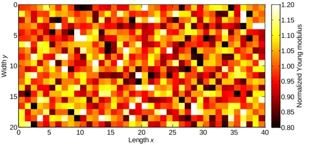
Figure 1-8. Moulded patch, detail of outer edge of repair [72]. 26 Figure 2-1. Map of a randomly distributed normalised Young's modulus over a composite lamina

with a mean of 1 (MPa/MPa) and standard deviation of 0.1. 37 Figure 2-2. Map of the distribution of the normalised Young's modulus spread over a composite

lamina with a known distribution where the mean NEx still equal to 1 with a standard

deviation of 0.1. 38

Figure 2-3. Map of the distribution of the Young's modulus spread over a composite lamina with a known distribution with random phase shifts. 39 Figure 2-4. Schema generation and assignment of elastic properties in the F.E. model, element per

element and ply per ply. 41

Figure 2-5. Challenges in the determination of the volume fractions of the constituent material at local scale (ply scale) and global (specimen) scale. 45 Figure 3-1. Typical cure cycle for a thick plate manufactured in M10.1/38%/UD300/CHS. 53 Figure 3-2. Prepreg M10.1/38%/UD300/CHS (view from below). 54 Figure 3-3. Determination of ply areas in protection scan of the image with, (a) the raw image after

the scan, (b) correcting the brightness and contrast, (c) binary image and (d) removal of black

(17)

Table of contents

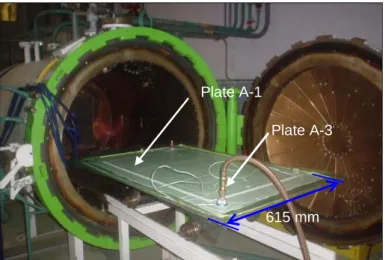
Figure 3-4. Mass per unit area compared to the area of the ply of samples E and R1. 60 Figure 3-5. Average of the mass per unit area for each specimen with ± 1 standard deviation. 61 Figure 3-6. Picture of the composite plates prior to introduction into the autoclave. 63 Figure 3-7. Diagram indicating the placement of thermocouples TC-1, TC-2 and TC-3 in the

composite plates. 64

Figure 3-8. Actual cycle of temperature for autoclave batches A, B and C. 65 Figure 3-9. Difference between the temperatures measured by thermocouples TC-1 and TC-2 to

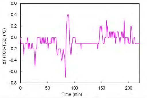
autoclave batch A and B. 66

Figure 3-10. Temperature difference between TC-2 and TC-3 thermocouples for autoclave batch B. 66 Figure 3-11. Schematic of vacuum bagging for the autoclave polymerization. 68 Figure 3-12. The batch “A” plates after being taken out from the autoclave and the excess flow of

resin impregnated the breather mat. 69

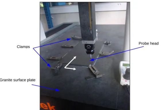
Figure 3-13. Positioning and clamping of a plate in the coordinate-measuring machine (CMM). 71 Figure 3-14. Schematic drawing of the profile of composite plates with, (a) with mosite and

(b) without mosite. 72

Figure 3-15. Reference system for the coordinate-measuring machine (CMM). 73 Figure 3-16. Thickness map of the A-2 plate. 74 Figure 3-17. Thickness map of the plate B-2. 74 Figure 3-18. Plate thickness generated using eq. 3-7. 75 Figure 3-19. Evolution of the volume fraction of the porosity through the plate thickness. 77 Figure 3-20. Evolution of the fibre mass per unit area ρAf with the ply thickness 78 Figure 3-21. Change of the volume fractions of the fibre with respect the plate thickness. 79 Figure 3-22. Change of the volume fractions of the resin respect the plate thickness. 79 Figure 4-1. DSLR Camera mounting on an adapted ceiling panel. 87 Figure 4-2. Working area (reference grid). 87 Figure 4-3. Fibre orientation measurement in a composite prepreg with, a) laid ply onto the work

zone, b) detail of an element image, c) the image after the application of the LOG filter and convolution masks, d) edge detection and e) Hugh lines along the fibre direction. 89 Figure 4-4. Precision test on the orientation method by Hough lines comparing the theoretical

value (written top) to the measured value (written between parentheses), each quadrant representing a different mean value with, (top) the 0° orientation and (bottom) the 45°

orientation. 91

Figure 4-5. Maximum resolution of the determined angle for a single Hough line according to the

maximum length of the image. 92

Figure 4-6. Mean number of Hough lines per elements (error bars for ±1 SD from the mean value) and its length in function of the number of elements with, (top) a ply oriented at 0° and

(bottom) a ply oriented at -45°. 93

Figure 4-7. Mean ply orientation in function the number of elements (error bars for a ±1 SD from the mean value) with, (top) a ply oriented at 0° and (bottom) a ply oriented at -45°. 95 Figure 4-8. Difference between the theoretical orientation and the measured orientation in the ply.

(18)

Figure 4-9. Orientation maps of 4 different plies from plate C-11 oriented, from top to bottom 0°,

+45°, -45° and 90° respectively. 101

Figure 4-10. Schematic description by a pseudo-Gaussian surface (on right) of a localized zone of fibre orientation perturbation (on left). 103 Figure 4-11. Comparison of the misalignment maps for the plate C-11 ply #15 oriented at -45° with,

(top) the measurements and (bottom) the ply reconstructed using the identification

algorithm. 105

Figure 4-12. Cumulative distribution function of the Amplitude Bi acquired by the optimisation

algorithm. 107

Figure 4-13. Cumulative distribution functions for the reconstructed misalignment using equation 5-2 (square markings) compared to experimental data (diamond markings) with, (top) the mean misalignment and (bottom) the standard deviation of the in-ply misalignment. 109 Figure 4-14. Cumulative distribution functions for the reconstructed misalignment using equation

5-2 (square markings), corrected for a zero mean (cross markings) compared to experimental data (diamond markings) with (top) the maximum values and (bottom) the minimum

values. 110

Figure 4-15. Localisation and amplitude of the 12 perturbation peaks used to generate digital in-plane misalignments, the diameter of the circles indicating the values of the amplitudes Bi

in degrees. 111

Figure 4-16. Map of the generated in-plane fibre misalignment with the size of the element of

30 x 30 mm. 111

Figure 5-1. Micrograph showing the ply thickness variations spread over a layered composite plate. 115 Figure 5-2. Mean ply thicknesses listed for each of the 16 plies ± 1 standard deviation, the measured

thickness divided by 2 for the pair of plies 4/5, 8/9 and 12/13. 119 Figure 5-3. Profiles for the #2 and #3 interfaces delimiting the #2 ply, the crosses showing the

selection points along the ply interface, while the continuous lines showing the interpolated

interfaces. 121

Figure 5-4. Thickness profile for the #2 ply and the least squares linear fit (dashed line) and the mean thickness fit (dashed horizontal line). 122 Figure 5-5. Profile of the plate thickness. 123 Figure 5-6. Zero mean thickness profile of the #2 ply before and after the application of a low pass

filter with a cut-off frequency of 1 Hz. 126 Figure 5-7. Amplitude spectrum of the thickness profile of #2 ply with selected frequency peaks.

127 Figure 5-8. Distribution of the number of peaks per ply (top) and amplitude distribution in

function of the frequency peaks (bottom) with the double plies 4/5, 8/9 and 12/13

considered as single plies. 128

Figure 5-9. Digital profile generated by the model with equation 1 compared to the real profile of

#2 ply. 131

Figure 5-10. Comparison of the CV between the real plies (diamond markings) and the generated

profiles (circle markings). 132

Figure 5-11. Representation of the cross section of the 16 ply stratification (plies 4/5, 8/9 and 12/13 shown as independent plies) with, a) reconstruction from the actual ply thickness profiles (after filtering), b) constant ply thickness accounting the contribution of the plate thickness variation in each ply and c) digital stratification generated by the proposed model. 134

(19)

Table of contents

Figure 5-12. Strain field of the upper skin of a 16-ply composite plate subject to a thermal of -120 °C simulating the cooling process of a composite (on the left hand side) with constant thickness and (on the right hand side) with variable ply thickness. 136 Figure 6-1. Map of the generated ply thickness in a ply of 200 x 100 mm dimensions. 145 Figure 6-2. Theoretical example of the reinforcement misalignment in a +45° 200 x 100 mm ply. 147 Figure 6-3. Theoretical example of a map of the Young’s modulus Ex distribution in a 200 x 100 mm

ply oriented at +45°. 148

Figure 6-4. Schema of the 4-point bending test with front view (top) and top view (bottom). 149 Figure 6-5. Load as function of the displacement in a 4-point bending test. 151 Figure 6-6. Flexural break load Pf of the tested specimens. 152 Figure 6-7. Composite failure in a 4 points bending test with (on the left hand side) the expected

failure of the 0° oriented plies under compression, and (on the right hand side) delamination

of the mid plane. 153

Figure 6-8. Flexural modulus Efx of the tested specimens. 153 Figure 6-9. Distribution of the flexural modulus Efx for a 16-ply laminate for a mean ply thickness

of 0.302 mm and standard deviation of 0.014 mm with (a) the plate thickness with the values x 16 (case 2); (b) each ply thickness different (case 3); (c) the ply thickness constant with ply misalignments (case 4) and (d) both the ply thicknesses and misalignments variables (case 5).

155 Figure 6-10. Strain field of the upper skin along the x-axis εx in a 4-point bending test for

Δsa = 3 mm (nose displacement). 157

Figure 6-11. Cumulative distributions for the flexural modulus of the 4-point bending test FE model for the deterministic case (dashed line), constant material properties (square markings) and material properties varying according to the local ply thickness (triangle

markings). 159

Figure 6-12. Comparison of the normalised flexural moduli as function of the plate thickness for 3 cases with constant thickness with ply thickness divided by 16 (cross markings), all

parameters variable (triangle markings) and experimental (square markings). 160 Figure 6-13. Thickness variation of the composite plate. 161 Figure 6-14. Thickness variation of ply #7. 162 Figure 6-15. Variation of the fibre misalignment in a ply (ply #4) with a theoretical orientation (at

+45°). 162

Figure 6-16. Nodal displacements w along the z-axis. 163 Figure 6-17. Strain field along the x-axis εxx for the upper skin ply#16 (top) and the lower skin ply

#1 (bottom). 164

Figure 6-18. Side view of the multi-axial testing machine. 165 Figure 6-19. Different loading scenarios possible with the actual configuration of the multi-axial

testing machine. 166

Figure 6-20. Composite evaluator to be tested in the multi-axial testing machine. 167 Figure 6-21. Boundary conditions in displacements imposed to the composite evaluator by mobile

clamp. 167

Figure 6-22. Composite evaluator during the testing, (right hand side) deformation of the plate in bucking moments before failure, (left hand side) failure of the composite, fracture of the outermost 0° ply subjected to compression near the clamp area. 168

(20)

Figure 6-23. Numerical representation by composite shell elements of the composite evaluator tested in a flexion-compression test. 169 Figure 6-24. Strain field along the x-axis εx for the lower skin of a technological evaluator in a

flexion-compression test with a homogenous material. 170 Figure 6-25. Strain field along the x-axis εx for the lower skin of a technological evaluator in a

flexion-compression test with material variabilities. 170

List of tables

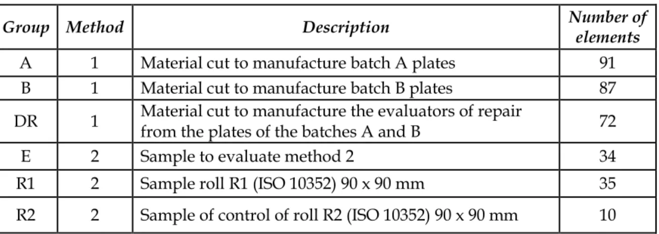
Table 3-1. Nominal properties of the prepreg s UD M10.1/CHS and M21/T700GC. 51 Table 3-2. Types, forms and formulas used for calculating the area. 55 Table 3-3. Identification of groups for the determination of the mass per unit area. 58 Table 3-4. Mass per unit area obtained with method 1. 59 Table 3-5. Mass per unit area of material lot L-1 obtained with method 2 samples. 59 Table 3-6. Summary of samples for comparison between the values of the MS for R1 and R2. 61 Table 3-7. Comparison between theoretical mass and the actual mass of the plates. 62 Table 3-8. Weighing composite plates before and after curing. 70 Table 3-9. Measurement of thickness of composite plates. 73 Table 5-1. Thickness comparison between the ply and the plate averages. 119 Table 5-2. Parameters of the distribution for the Frequency (uniform) and Amplitude (normal)

associated with the probability of appearance of the ith peak within a frequency band. 130 Table 5-3. Frequencies and amplitudes of the thickness evolution for the digital stratification. 131 Table 6-1. Homogenized elastic constants necessary for the composite shell element according to

the SAMCEF® software syntax. 143

Table 6-2. Mechanical properties of the CHS reinforcement and M10.1 resin. 143 Table 6-3. Measurements and calculations coming from the 4-point bending test. 152 Table 6-4. Statistical values of the plate thickness and flexural modulus Efx. 155 Table 6-5. Elastic quantities for the principal directions 1 and 2 calculated for the median ply

thickness of 0.300 mm. 156

(21)

(22)

(23)

General introduction

The employment of composite structures in transport and civil applications has shown an exponential growth during the last decade. Today, the aeronautical industry relies heavily on the use of these advanced materials to decrease the structural weight and maintenance costs associated to corrosion and fatigue. However, polymer matrix composite materials present a higher variability of their mechanical properties compared to the classic engineering materials, such as metals. The origins of the material variability can be traced from the elementary material variability, the manufacturing conditions and chosen geometries of the composite structure, thus the notion of variability cannot be dissociated from the finished product. From the point of view of a finite element model, the input parameters that modify the structural behaviour include, but are not limited to the volume fractions of the fibres, resin, and porosity; the fibre orientation, both in-plane and out-of-in-plane, characteristics of the type of material of the reinforcement and resin system employed, etc. In fact, the list of parameters and its couplings at the different material scales can be considered infinite, adding an unknown complexity to the composite solution. A first step to address the problem is through the geometric description of the composite structure at the mesoscopic and structural scales. This geometric description is driven by the evolution of the thicknesses of the plies and the structure itself.

For design purposes, the structure thickness is given by the sum of the ply thicknesses that form the laminate, or alternatively the thicknesses of the plies are obtained by dividing the total structure thickness by the number of plies of the given stratification. The thickness of the structure is thus considered as constant and equal for all plies, provided that there is not change of the geometry of the

(24)

cross section and stratification. In reality, each ply in the stratification does not present a constant thickness (cf. Figure 1).

Figure 1. Micrograph showing the ply thickness variations spread over a layered composite plate.

The main goal of our approach is to propose a finite element model that takes account of the geometric and material variability present in a composite structure. This model is based on the assumption that the property variation shows a continuous evolution through the composite dimensions that cannot be reproduced by only randomly assigning a set property to each element of the model.

This dissertation is composed by six chapters.

The Chapter 1 is dedicated to a literature review where the variability parameters are shown to be tightly linked to the manufacturing process of the composite plate, as well as the raw materials.

In Chapter 2, an overall solution for the variability introduction into a FE model is proposed.

(25)

General Introduction In Chapter 3, the general process of fabrication and measurement of the sources of variability are described for a chosen composite plate, with a particular focus on the measurement of the following parameters.

The mass per unit area of the composite prepreg is a parameter associated with the variability of volume fractions of the elementary constituents. The influence of resin flow during the polymerisation by weighing the plates before and after the cure cycle is considered. The plate thickness variation through the composite plate and the differences that are due to the sequence of the used vacuum products in different autoclave batches are taken into account. It deals with the determination of the volume fractions of the constituent materials of the cured plates.

In Chapter 4, the reinforcement misalignments are quantified during the lay-up procedure of the prepreg plies. A more in-depth analysis on the evolution of the ply thickness variations and the fibre orientations, describing the methods to obtain the geometric properties and as well the mathematical laws for their modelling is described. In a first step, the difference between the actual orientation and theoretical orientation of the plies is obtained. Then by the implementation of an in-house program, the values of local misalignments are determined.

In Chapter 5, the evolutions of both the ply and the plate thicknesses are quantified. Using images of the cross-section of the composite, the variations in the thicknesses are modelled. It is demonstrated that the profile of the ply thickness exhibits a periodic variation. The amplitude spectrum, obtained by a discrete Fourier transform of the thickness profile, is then used to determine the representative pairs of frequencies and amplitudes. These representative peaks are used to model a digital ply that has variability of the same order of magnitude as the measured thickness profiles.

Finally, in Chapter 6 three cases of FE model are considered using the methodology proposed in Chapter 2 and the mathematical laws proposed in Chapters 3 through 5.

(26)

(27)

Chapter 1: Literature review

1.1 Introduction

Variability in composite materials is referred to the dispersion of the properties that these materials exhibit, and such are much more significant than for classic engineering materials, like the metals. The Military Handbook 17 [1] states that the variability of the composites property data may originate from different sources, like batch to batch variability in raw materials, variability in the fabrication process of the composite part, variability during the testing and the intrinsic variability of the material. However, in the literature, the definitions of variability and uncertainty are often used indifferently, as they are included within the boundaries of the lack of knowledge of the system [2].

1.2 Definition of variability

Thunnisen [3] made a recompilation of different definitions of uncertainty grouped by areas of knowledge. In this recompilation, he states that there is no agreement in the different terms that are understood under the term uncertainty, the variability being one of these definitions. Likewise, he found that different areas of knowledge assign a different classification and term definitions for the same words. For the mechanical engineering domain, one of the most suitable taxonomy of the systems uncertainty is offered by Oberkampf [4], in which the variability is defined as the inherent variation associated to the physical system under consideration. Meanwhile, the uncertainty is the potential deficiency in any

(28)

Chapter 1

phase or activity of the modelling process due to a lack of knowledge or incomplete information. Finally, an error is a recognisable deficiency in any phase or activity that is not due to the lack of knowledge. As can be seen, it is extremely difficult to draw the line between each definition, especially when dealing with multilevel systems with complex interactions such as the composite materials.

Therefore, the material variability can be defined as the dispersion of properties that are due to the spatial and consistency variations of the material itself, and due to variations in its processing. The components of the material variability can be the combination of fixed effects and random effects and as well as errors. The fixed effects are produced by the controlled variables which are a systematic shift in a measured quantity due a particular level change or a treatment or condition, which is often under the control of the experimenter. The random effects are produced by uncontrolled variables that produce a particular change in the measured properties. This random effect is never under the control of the experimenter. The shift in the measured quantities is viewed as a random variable with a zero mean and a non-zero variance. The errors are the part of the data that varies due to unknown or uncontrolled external factors that affect the observation independently and unpredictably. A random error is a special case of a random effect where the errors vary independently from measurement to measurement. To further classify the errors, they can be divided into acknowledged and unacknowledged errors. An acknowledged error is for example the approximations or assumptions to simplify the modelling of a physical process, meanwhile an unacknowledged error can be referred as a simple mistake [3]. Defect is another term that is usually found in the literature linked to experimental work. A defect can be defined as an involuntary split, or flaw, from the theoretical properties produced by a physical imperfection of the material or caused by an error during the composite part processing.

In order to successfully design a composite structure, the reliability of the system must be demonstrated. This exercise consists in the evaluation of the probabilities for the various structural responses to satisfy the specified design

(29)

Literature review criteria and quantify the uncertainty ranges for each response. The scatter in the structural behaviour cannot be simulated by the traditional deterministic methods that use a safety factor to account for uncertain structural behaviour. A probabilistic method is thus needed to accurately determine the structural reliability of a composite structure [5, 6].

Effectively, the vast quantity of variabilities and the infinite possible effects make difficult the calculation and analysis of composite structures. There are multiple methods and approaches that can be used. The acknowledgement of variability is therefore limited to the fields of study and the expected results. This implies that there is no global framework to introduce the variability in composite structure design.

The properties of composite materials are cure and process dependent. In most of the cases, the composite structures are the product of complex multi-step procedures, and with each step, additional variability is introduced [7]. One important point to take into consideration is that most of the work done to design a composite structures is based on the test pyramid [1]. Thus, the design properties of composite material are derived from small laboratory scale coupons. It has been thought that when increasing the size of the composite its strength decreases. This is based on the assumption that the probability of encountering a flaw large enough to initiate the structural failure increases with the size of the specimen. However, this is not necessarily true since the processing techniques to fabricate a test coupon are not the same as those used to fabricate as full scale structure [8].

As is often the case, there is a strong dichotomy on the calculation aspects of the composite structures and the compilation of data in a real composite structure. This literature review intends to cover, on one side, the general aspects on how the variabilities in composite materials are studied during the design and analysis phases, and on the other side the lack of actual properties of the composites materials. The first part of this review is dedicated to the analysis and design of composite structures; starting from the most used methods to the required data

(30)

Chapter 1

that is introduced into the models. The second part of this review focuses on the sources of variability of the real composite material and the techniques used to measure the material properties.

1.3 Variability calculation of the composite materials

1.3.1

Introduction to a stochastic design of composite materials

The analysis of composite materials is performed usually at three different scales of the material: at the level of the elementary materials (fibre and matrix), known also as micromechanical level; at level of the homogenised ply or meso-scale, and at the structural scale, also known as macromechanical scale. Sriramula and Chryssanthopoulos [9] considered a significant number of studies and classified them into these three major groups regarding the scale at which the material is observed. The class A is set at micromechanical level, and it is further divided into two subgroups:

The class A1 deals with the analysis of the composite from the determination of the material properties by the use of the micromechanical structure of the composite. In this class, the identified probabilistic models for the random variables can be introduced into composite micro-mechanics theory, leading to effective property estimation at lamina level, which can be later combined with the laminate theory and finite element (FE) analysis [10].

The class A2 builds the micromechanical properties from the morphology of the composite microstructure by the use of sophisticated numerical modelling of microstructural randomness in conjunction with spatial variability modelling of the studied variables. These methods consider of a representative volume element (RVE) of the composite structure linked to an appropriate micro-mechanical model to evaluate the response behaviour (cf. Figure 1-1). An example of a class A2 methodology is given by Guillaumat and Dau [11,12] where, using a micrograph of a composite cross-section, a RVE of the composite is determined.

(31)

Literature review Then, by varying the diameter of the fibres and the elastic moduli of the fibres and matrix, as well as the Poisson’s ratio for each variable, the compliance matrix of the composite lamina is determined. To reduce the impact of uncertainties at this stage, a material database is stablished to show the admissible and non-admissible values for each property at any given scale [13].

Figure 1-1. Uncertainty modelling and propagation in Class A2 approach [9].

Class B problems are studied at a component level (composite beam or panel). In this case, the models are based on random variables based on experimental evidence and engineering judgment. Typically the probability distributions for random variables representing stiffness or strength properties are specified. Finally, the meso-scale modelling, or Class AB, which is an intermediate stage of modelling, is suggested when the ply characteristics significantly influence the composite properties. This class is also used to verify the propagation of uncertainties across the length scales.

(32)

Chapter 1

The rational treatment of the great number of variables considered in a composite system can be achieved by means of probability theory and statistics, and cannot be addressed by the traditional deterministic approach. Stochastic methods provide a way to represent a wide range of structural loading and strength scenarios. A stochastic field is defined as:

 



x



F x

F( ) 1 (1-1)

where the stochastic response of a variable F(x) is described by the mean value of said variable F̅ and a zero mean stochastic field ξ(x). There are two major approaches to assess a composite structure through a stochastic framework: reliability based methods and stochastic finite element methods (SFEM). For both approaches, the Monte Carlo simulation (MCS) is the most used method to solve stochastic problems and serves as well as a benchmark to qualify the results obtained by other types of methods [14].

As an example of a stochastic method to analyse composite structures presenting variability, Venini [15] used the Rayleigh-Ritz method to study an out-of-plane vibration of a cantilever composite beam. In this problem, five zero-mean random fields are introduced at a macromechanical level (E1, E2, ν12, G12, and the material density ρ). The properties were modelled as homogeneous

random fields to be averaged into random variables by means of the stochastic Rayleigh-Ritz method, where each random variable results from a spatial average over the whole domain of the structure and therefore is representative of the entire structural system.

1.3.2

Reliability based methods

The reliability is defined as the probability that the system performs its intended functions for a specific period of time under a given set of conditions. In other words, the reliability is the probability that unsatisfactory performance or failure will not occur.

(33)

Literature review The probability of failure Pf is:

 









_

_{ }_

 

 0 0 x G X f PG x f x dx P (1-2)

where fX(x) is the joint probability density function (PDF) of the random variables

X, whose realisations are x, and G(x) ≤ 0 denotes the failure domain. The reliability index β is the shortest distance between the origin of the space and the failure domain in the normalised space (cf. Figure 1-2).

Figure 1-2. Schematic representation of FORM/SORM approximations [16].

A first order reliability method (FORM) is used to approximate the boundary of the failure domain G(x) into a linear function, by means of a first order Taylor series approximation of G(x) in the vicinity of the design point to evaluate the β index. A second order reliability method approximates the failure domain using the second order derivatives of G(x).

The strength of a fibre reinforced in a composite material can be adequately described by probabilistic methods. Soares [17] introduced the different probabilistic approaches to represent the strength of fibre reinforced composite materials and to assess the reliability of laminated components. Di Sciuva [14] compared the mechanical properties of a composite beam obtained by MCS and several algorithms. In this study, the deformation of a cantilever composite beam

(34)

Chapter 1

is calculated using stochastic variables which are the moment of inertia J, the Young’s modulus E, the length of the beam L and the transverse load applied to the beam q. Using a convergence criterion pre-established, they determined both the maximum deflection of the beam and the reliability. It is evident that FORM algorithms offer quick convergence and low computational costs.

A probabilistic approach can be used to construct the macroscopic properties of a composite plate from the constituent materials to obtain a stochastic response of the macroscopic properties. Shaw et al. [18] used 14 random properties of the elementary constituents of a composite plate obtained from the literature to determine the macroscopic properties of the studied plate. By using MCS the macroscopic properties of the composite plate were then obtained. The properties include the longitudinal and transversal moduli in the principal directions, E1 and E2, the shear modulus G12 and the Poisson’s ratio ν12, as well as

the ultimate longitudinal and transversal stresses, XT and YT. The derived

macromechanical properties were compared against three probability distributions to determine the most suitable distribution for each property using a Kolmogorov-Smirnov (K-S) goodness-of-fit test. The tested probabilistic laws were the Normal law, the 2-parameters Weibull distribution and the lognormal (L-N) distribution. The failure probability estimates were then calculated by a combination of MCS and FORM/SORM using the Tsai-Hill failure criterion. Although this study compares the macroscopic properties derived from the micromechanical analysis to the values obtained by experimental setups found in the literature, it does not takes into account neither the details of the used material system, other than being a carbon/epoxy, nor the fabrication process. In comparison, Lekou and Philippidis [19,20] created a material database obtained from the tensile test coupons. The E-glass/polyester coupons were fabricated by hand lay-up. Nine macroscopic properties were obtained by experimental means. Each property was compared against 6 probability laws using the K-S test and the Tsai-Hahn criterion is used as a limit state function.

(35)

Literature review The reliability methods are used also to obtain the sensitivity factors of certain variables and how they affect the global behaviour of the system. Antonio [21] used MCS in a global sensitivity analysis to determine the reliability of a composite plate. The parameters used to assess the reliability were the maximum displacement and the critical Tsai number covering four stochastic variables: the ply angle, the elastic strength, the lamina thickness and the loading of the composite. The study assesses the effect of each property at different ply angles, ranging from 0 to 90°. The material properties are obtained from the literature and the coefficients of variation of each property are assigned.

1.3.3

Optimisation methods

The variability of the composite material does not only impact the reliability of the structure, but also it must be taken into account in the optimisation phase of the composite structure.

Walker [22] developed a technique for optimally designing fibre-reinforced symmetric laminated plates under buckling loads for minimum mass accounting for manufacturing uncertainties in the fibre layup orientation. The constraint implemented is a minimum buckling load carrying capacity constraint, and the objective is to determine the value of the fibre orientation that corresponds to a minimum plate thickness, with the uncertainty included.

Correspondingly, the optimisation techniques can be coupled with reliability analysis. This is the case of cylinders subject to pressure. Boyer and Béakou [23,24] obtained the optimal winding angle which reduces the mass of the composite structure by maximising the distance between the operating point and the failure domain. The failure mode used in this study is the Tsai-Wu criterion. The mechanical properties of the composite are built from the micromechanics of the elementary materials, using 9 properties with values obtained from the literature. Bouhafs et al. [25,26] expanded on the study of pipes to the sensitivity analysis of the design parameters, within a macromechanical study. This time the

(36)

Chapter 1

variable parameter was the thickness variation of the container. Khiat et al. [27] continued with the micromechanical level by studying the fibre arrangement and analysed the sensitivity against the failure criterion, that in this case is the ineffective length of the broken fibres. A sensitivity analysis is performed to see how the probability distribution of the behaviour response changes when adding the stochastic parameters. The mean response remains the same, but the tails of the distribution function are more spread, indicating a higher value of uncertainty (cf. Figure 1-3).

Figure 1-3. Probability distributions of the ineffective length for various combinations of random variables [27].

Composite materials show a wide variety of failure mechanisms as a result of their complex structure and manufacturing process. The accuracy of the reliability analysis is critically dependent on the appropriate criterion for the study conditions. Moreover, the reliability methods can be used to provide a reliability-based calibration to define the safety factors in the composite structure [16].

(37)

Literature review

1.3.4

Stochastic finite element methods

Previous works are oriented into obtaining an analytical solution to the reliability calculation of composite structures. Therefore, they have their limitations on the size and the shape of the structure to be analysed. The FE analysis is a powerful tool to study the behaviour of complex structural systems. A stochastic finite element modelling (SFEM) implies that the values at each element are stochastic in nature, leading to random properties [28]. Computer power has grown at an increasing pace during the last few years permitting the SFEM to resolve large scale problems.

Mendoza-Jasso [29] studied the open hole off-axis test of a unidirectional IM7/8552 carbon epoxy composite. In this case, the macromechanical properties

E1, E2, ν12 and G12 were treated as stochastic variables, with their values varying for

the entire coupon. A local variability of the fibre volume fraction Vf is introduced

in bands aligned with the fibre axis. Vf of 0.556 with 2 different standard

deviations of 0.03 and 0.09 are evaluated. The value of standard deviation was obtained from experimental data. Their results show that the dispersion in the fibre volume fraction is one of the causes of the probabilistic distribution of the failure initiation location in the coupons tested experimentally. The SFEM analysis of complex structures can be coupled with a first-order reliability approach [30]. This approach is applicable to any limit-state criterion that is prescribed in terms of random variables. Measurements of reliability sensitivity with respect to any set of parameters can be easier computed than with MC Simulation.

SFEM is a particularly powerful tool to assign at each element a different property, as shown by Spanos [31]. In this study that deals with single-walled carbon nano tubes, a methodology to assign a different element property to composite plate is introduced. The most used method to deal with the response variability calculation is the Monte Carlo simulation [28]. The mechanical properties are derived from MCS of the volume fraction of the reinforcement at each element. The MCS is the easiest method since it does not require a reformulation of the deterministic formulation of the FE analysis in order to take

(38)

Chapter 1

account the random field. Thus, the homogenised properties can be used to determine the local Young modulus and the local Poisson’s ratio. The volume fractions of the reinforcement were obtained from the micrographic observations. Thus, the values obtained are representative of the reality of the composite plate.

Regardless of the type of analysis to be performed, whether analytical or SFEM, in the majority of cases, the statistical data used as model input assumes that the mechanical properties are independent from the manufacturing process. Indeed, many of the structural performance calculations are based on the data obtained from elementary coupons. When changing the scale and the size of the tested element, the mechanical properties do not correlate with the model prediction. This is often linked to the increased probability of finding a material defect that initiates the failure. However, as Sutherland [32] suggested, the conditions of manufacturing of test specimens having larger dimensions are different from those employed to produce elementary coupons. Thus, the scale of the composite, as well as the fabrication process, must be taken into account when building a material database in order to feed stochastic models.

In order to better understand how the different sources of variability affect the composite structure, another literature survey is performed. This time, the focus is put on the actual manufacturing and how the measuring techniques affect the material properties.

1.4 Identification and quantification of the variability

during the manufacturing of composite structures

1.4.1

Interdependencies of the sources of variability of composite

materials

As stated, composite materials are the product of multiple complex processing stages to form the composite structure. Each stage adds its own variables that affect the material in various forms. This makes the problem even