Measurement of the Dark Energy Equation of State Using the Full SNLS Supernova Sample

(1)

HAL Id: tel-01127401

https://tel.archives-ouvertes.fr/tel-01127401

Submitted on 7 Mar 2015

HAL is a multi-disciplinary open access

archive for the deposit and dissemination of sci-entific research documents, whether they are pub-lished or not. The documents may come from teaching and research institutions in France or abroad, or from public or private research centers.

L’archive ouverte pluridisciplinaire HAL, est destinée au dépôt et à la diffusion de documents scientifiques de niveau recherche, publiés ou non, émanant des établissements d’enseignement et de recherche français ou étrangers, des laboratoires publics ou privés.

Measurement of the Dark Energy Equation of State

Using the Full SNLS Supernova Sample

Patrick El Hage

To cite this version:

Patrick El Hage. Measurement of the Dark Energy Equation of State Using the Full SNLS Supernova Sample. Cosmology and Extra-Galactic Astrophysics [astro-ph.CO]. Université Pierre et Marie Curie - Paris VI, 2014. English. �NNT : 2014PA066382�. �tel-01127401�

(2)

DOCTORAL THESIS

OF THE UNIVERSITÉ PIERRE ET MARIE CURIE

presented by

Patrick El-Hage

To obtain the title of

DOCTEUR EN SCIENCES

DE L’UNIVERSITÉ PIERRE ET MARIE CURIE

Measurement of the Dark Energy Equation of State

Using the Full SNLS Supernova Sample

To be defended to the following jury on September 26th_{, 2014 :}

Julien GUY Thesis advisor

Rick KESSLER Referee

Emmanuel BERTIN Referee

Christophe YÈCHE Examiner

Jacques DELABROUILLE Examiner

Michael JOYCE Examiner

(3)

(4)

A little knowledge that acts is worth infinitely more than much knowledge that is idle. Gibran Khalil Gibran

(5)

(6)

Acknowledgements

My journey at the Laboratoire de Physique Nucléaire et de Hautes Énergies (LPNHE) began a few months before my thesis did, during my Master’s degree (NPAC) internship. My first memories at the laboratory are those of Julien Guy and Pierre Astier talking over each other in an attempt to explain to me the objectives of my internship. In the short hour I spent with them, I was bombarded with details on topics ranging from supernova cosmology as a whole to the finer details of manipulating a Fisher matrix for optimization purposes. Needless to say, I left that office confused and intimidated. That meeting, however, set the tone for the next 3 years of my life, in that the LPNHE cosmology team would treat me not as an underling but as a colleague, albeit a slightly inexperienced one.

After that first encounter with the dynamic duo of French cosmology, my circle of collab-orators would only grow. While my own research often focused on minute technical details, I could always count on the rest of the group for friendly discussions regarding broader topics in cosmology. Here I would like to thank in particular Pierre Astier, Nicolas Regnault, Sébastien Bongard, Laurent Le Guillou, and Augustin Guyonnet for the time they took in imparting some of their technical expertise regarding the bigger picture of supernova cosmology. I would also like to thank Reynald Pain, our fearless leader, for his wisdom regarding the challenges and out-looks of being a graduate student and his frank discussions of the current state of fundamental physics.

As time progressed, so too did my reponsabilities as a member of the SNLS collaboration. As the third year of my thesis came around, it was time for me to process and analyze the final SNLS supernova sample. Here I must extend my sincerest gratitude to Marc Betoule for his time, patience, and software, all of which greatly facilitated this part of my reaserch. In particular, by exploiting his previous experience with the JLA anlaysis he allowed me to focus my attention on the more pressing scientific questions I was facing rather than spend time dealing with pipeline issues. His help in this regard was so significant that I was even willing to overlook his unintelligible code writing style. Here I would also like to thank Delphine Hardin and Christophe Balland for their crucial help in core aspects of the SNLS analysis, in particular for having adapted their timelines to my thesis requirements despite their exceedingly busy schedules.

Throughout it all, there was my advisor, Julien Guy, whose enthusiasm for science and all its gory details can only be described as infectious. During our time together he has done more than merely invigorate my passion for cosmology, though he has certainly done that as well. I knew that I was always welcome in his office, and as such we would regularly discuss matters ranging from the direction of my thesis to the optimal choice of revision control software for our next project. Indeed, we regularly spent hours on the same computer screen, often times even passing the keyboard back and forth to each other. In those moments he imparted upon me a

(7)

Acknowledgements

work method that will stay with me well beyond my years as a graduate student. While a love of science is commonplace, Julien has taught me how to love details without drowning in them, and how to appreciate the importance of expertise without ever forgetting the bigger picture.

I would like to add that while Julien was my official thesis advisor, both Marc Betoule and Pierre Astier were also a constant source of support during my thesis, despite having no formal obligations towards me whatsoever. In addition, help came from well beyond the walls of the LPNHE, as the many international researchers I had the opportunity to collaborate with proved to be a rich source of intellectual stimulation. In particular, I would like to thank Rick Kessler for his warm welcome during my visit to Chicago.

Beyond the cosmology team, there were many people that made the LPNHE the welcoming environment that it was. I would like to thank Véronique Joisin, Vera Varanda, and Magali Carlosse for their organizational efforts which make the life of an LPNHE researcher possible, as well as François Legrand, our systems administrator, for always helping me out when I was in a bind. During my years at the LPNHE, Eli Benhaim was my graduate “godfather”, a job he took very seriously by regularly checking up on me to ensure that all was well. He provided me with a safe space to air both my joys and my concerns with regards to the progress of my thesis, and for that I am very grateful. I would also like to thank Sophie Trincaz-Duvoid both for her help during my Master’s degree, as well as the support she shows all graduate students of the LPNHE.

Of course, no graduate student experience would be complete without other graduate stu-dents who suffer alongside you. I would likely not have survived these last 3 years were it not for the friendship and solidarity of my fellow NPAC graduates, as well as the students I befriended along the way. While it may have led to a diploma, it would have been a sad thesis indeed with-out the cheerfulness of Guillaume Lefebvre, Aurélien Demilly, Pierre Morfouce, Agnès Ferté, Matthieu Roman, and Tania Garrigoux.

I would not have even contemplated pursuing my passion without the constant support of my family. I would not be the passionate geek I am today were it not for my brother and the childhood we spent building legos together. Today, my sister is the biggest fan of my work, despite not understanding much of it, and I am eternally grateful for her fascination with the universe which serves to remind me of the ultimate purpose of scientific pursuits. Of course, were it not for my parent’s encouragement that I pursue my dreams regardless of how odd they seemed to those around me, the very concept of becoming a cosmologist would not have even occured to me. And while we may not be technically related, Raja Salamé’s unwavering friendship is what has allowed me to enjoy the ride in this pursuit, and to me that makes him as good as family.

This pursuit was also greatly aided by a number of scholarships. The first of these was the Philippe Jabre scholarship which allowed me to attend the Research Science Institute at MIT while still in high school. The second was the Fayez Sarofim Scholarship which covered the complete cost of my undergraduate tuition while at Rice University. And finally, the last of these was the French government grant that made this thesis possible. I will strive for a career as a researcher that lives up to the expectations of these financial benefactors.

Also during that pursuit, I encountered many professors which played a crucial role in making me the person I am today. I will start by thanking Jean Baptiste Fourest, my middle school math teacher, for teaching me that a passion in life is something to be treasured and nurtured. I would then like to thank professor Paul Padley for introducing me to the world of research by granting me the opportunity to work at CERN for a summer, as well as his willingness to talk about life and all things physics during his invaluable office hours. I would also like to thank

(8)

Acknowledgements everyone at NPAC, teachers, students, and administrators, for making me feel so welcome when I first got to France, as well as for their availability in my times of need.

Last, and most certainly not least, special mention must be made of the role Laura Cottard played in shaping my academic career. Had I not decided to follow her to France after graduating from Rice University, I would not have discovered NPAC. Had I not discovered NPAC, I would not have discovered cosmology, the field that I was always meant to pursue. Had I not pursued cosmology, I would have likely ended up in the field of particle physics, or worse yet in applied physics. On the whole it goes to show that even when it tells you to cross an ocean, your heart always knows best.

(9)

(10)

List of figures

1.1 Here we plot the observed flux of an object as a function of the redshift at which its light was emitted, for different cosmology models. The dashed line corresponds to a flat matter dominated universe in which there is no acceleration. The solid line corresponds an accelerating expansion, similar to actual observations. . . . 11 1.2 The density profile required to explain the observations implies the presence of

significant amounts of missing mass. . . 12 1.3 Cosmological results using the luminosity distance estimates ofPerlmutter et al.

(1999). . . 14 1.4 Map of CMB temperature anisotropies as seen by Planck. The central regions

correspond to the galactic plane and are mostly excluded from cosmological anal-ysis. . . 15 1.5 Uncertainty contours of the JLA analysis. “Planck” represents CMB temperature

data, “WP” represents CMB polarization data, and “BAO” represents BAO data. Note that in both parameter spaces, the 2 contours are nearly perpendicular and greatly compliment each other. . . 17 1.6 Uncertainty contours in the w VS wa plane provided by the JLA analysis. wa is

almost completely unconstrained. . . 20 2.1 Spectroscopic properties of a typical SNIa. Note that the emitted flux peaks in

the blue band. For this reason, we establish the convention that the integrated flux in this band is to be used when comparing supernovae. . . 22 2.2 Typical supernova lightcurve, before and after model fitting, of supernova 03D4ag

from the SNLS5 analysis. Note the second smaller peak in the redder i and z bands. 23 2.3 The 2 most visible correlations between SNIa brightness and lightcurve properties. 24 2.4 Spectra and light-curves of peculiar SNIa relative to normal SNIa. The differences

between the two are less obvious then between Ia and non-Ia supernovae, but are still significant enough to be distinguished after careful consideration of all the information at hand. . . 25 2.5 Total transmission functions for the 5 filters that describe the SNLS data. Tais the

atmospheric transmission function, Tm is the instrument transmission function, T0 is the filter transmission function, and ‘ is the quantum efficiency of the CCD.

The total transmission function is the product of all of these. . . 28 2.6 . . . 30 3.1 The objective is to compare the supernova fluxes highlighted in blue. The left

hand figure shows us how to calibrate fluxes, whereas the right hand figure shows the necessity of a spectrophotometric model of SNIa. . . 36 3.2 Location of the wide and deep fields in the night sky. . . 37

(15)

List of figures

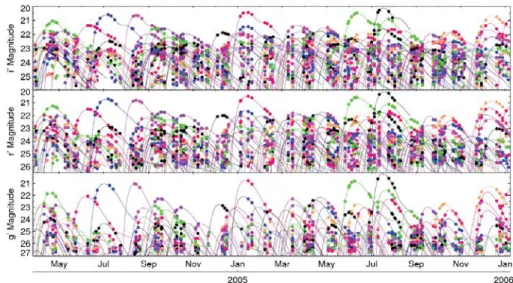
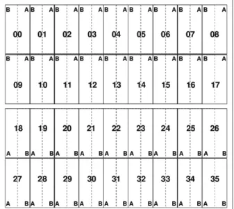
3.3 SNIa candidates, detected between May 2004 and January 2006, and their bright-ness in g, r, or i band as a function of time. . . 40 3.4 Telescopes used for spectroscopic confirmation of SNIa candidates for the SNLS. 41 3.5 The MegaPrime instrument (from the CFHTLS website). . . 42 3.6 Arrangement and numbering scheme of the CCD mosaic. A and B correspond

to the 2 amplifiers used during readout. Taken from Terapix. . . 44 3.7 Effective model of the optical path within the MegaPrime instrument. The

model’s free parameters include the properties of each lens, the distance from one lens to the next, and also an offset between the lens center and the central axis, in order to model the impact of misalignement of the various components. Taken from Villa(2012). . . 44 3.8 Example of the end result on the CCD of illumination of the focal plane by a given

LED. The deformed square near the middle is the result of inner reflections. Taken from Villa (2012). . . 45 4.1 Gaussian-weighted second moments from a single typical image, with the found

star clump and the star selection (red points within the ellipse). . . 50 4.2 Astrometric 1-D residuals scatter as a function of star magnitude for the D3 field

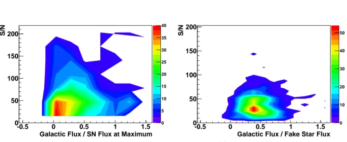
in r band. The top plot compares, as a function of magnitude, the measured residual RMS (points) with the average expected RMS (curve) including a noise floor of 0.013 pixels. They are roughly compatible, but not necessarily equal because the expected RMS varies with IQ at fixed magnitude. The bottom plot displays the RMS of the residual pulls (i.e. residuals in unit of expected RMS), which are close to 1 at all magnitudes. We hence conclude that adding the position noise floor of 0.013 pixels (2.4 mas) in quadrature to the position uncertainty expected from shot noise fairly describes the residuals. This figure only considers residuals along y for reasons explained in section §4.2.3. . . 53 4.3 . . . 57 4.4 Above are density plots comparing the distribution of real supernovae and

simu-lated fake stars in the plane of S/N of the supernova lightcurve VS the ratio of the galaxy flux to the supernova flux at maximum. . . 60 4.5 Photometric factor accuracy as a function of S/N for the RSP method. We have

binned the estimated ˆr/r in S/N bins. We plot both the uncertainty on the bin mean as well as the dispersion in the bin so as to compare it to the expected dispersion at that S/N. We also plot the expected S/N bias, as well the obtained fit for equation 4.14. . . 62 4.6 Photometric factor accuracy as a function of S/N for the DSP method. We have

binned the estimated ˆr/r in S/N bins. We plot both the uncertainty on the bin mean as well as the dispersion in the bin so as to compare it to the expected dispersion at that S/N. We also plot the expected S/N bias, as well the obtained fit for equation 4.14. . . 62 4.7 . . . 63 4.8 Standard deviation of flux estimates over the lightcurve as a function of the

average flux. The relation is shown here for high-flux field stars, and we see a clear linear relationship, indicative of a contribution to scatter beyond shot noise from the sky and the object. . . 64

(16)

List of figures 4.9 We plot here the ratio of the modeled uncertainty to the RMS of the light curve,

as a function of the sum of the fluxes of the fake star and galaxy. The two set of points refer to before and after adding a — term to the model uncertainty (Eq.

4.16). We see that the correction makes only a small difference. . . 64

4.10 Evolution of ‰2_/N_dof _{of night fits of real SNe as a function of redshift. . . .} ₆₅

4.11 We consider the error in the fitted position in units of ‡IQ as a function of the S/N ratio. We also plot the expected relation between the two using equation 4.17. 66 4.12 To fit the form factor, we fit a slope in the r2 _{VS flux bias plane, where r is} the error on the position. Each black point represents the computed bias using equation 4.18 for a random position on the image and a random displacement across it. . . 66

5.1 The solid black lines represent the old calibration transfer scheme, as described in Regnault et al. (2009). The dotted red lines represent the work done in Betoule et al.(2013). The instrument names indicate that both sets of stars were observed with the said instrument, hence making flux calibration transfer possible. . . 70

5.2 Relative corrections to the twilight flat fields due to grid corrections. . . 71

5.3 Overview of the MegaPrime photometric response analysis. Boxes describe the various data sets involved in the construction of the model (dashed for external data). Ellipses represent the main steps of the analysis. Taken fromBetoule et al. (2013). Using the lessons learned from surveys such as SNLS and SDSS, newer surveys such as DES and LSST will regularly measure the combined impact of the optics, the filters, and the CCDs rather than dealing with them separately. . 72

5.4 Filter induced color dependence of magnitudes at 17cm from focal center in u, g, r, i, i2, and z bands. . . 73

5.5 Ratio of the fitted sky level to the flux of the star as a function of color, for high flux stars only in i band. For such stars we assume that the fitted sky level is predominantly a fraction of the flux incorrectly fitted as the sky level. We see that the fraction of flux that goes into our sky level estimator evolves linearly with color. . . 75

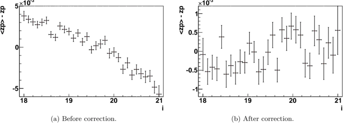
5.6 Plot of zero point residual vs magnitude in i band, before and after correcting for aperture sky pollutions. . . 76

5.7 Comparison of data with Pickles (1998) spectroscopic library in order to fit an appropriate effective filter, in g band. . . . 78

6.1 Distribution of the full supernova sample (before cuts). . . 83

6.2 . . . 85

6.3 Evolution of standardization parameters as a function of redshift. . . 87

6.4 Diagrammatic overview of the simulation process. We begin by choosing the un-derlying input models for both the cosmology and the supernovae. This produces two sets of supernovae : one for SALT2 training, and one for cosmology. Once the training is complete, distance moduli are computed for the cosmology set. In turn, we correct these moduli for Malmquist bias, and fit a cosmology to them. We can then compare the input and output values of the cosmological parameters, in particular w. . . . 88

6.5 Difference between input and recovered distance moduli for various input models. The first two entries in the model name describe the input spectral and intrinsic scatter models. The last two indicate that a “real” training set was used. . . 89

(17)

List of figures

6.6 Fitting galaxy mass VS KS magnitudes. . . 91

6.7 Hubble residuals as a function of galaxy mass, before any correction is applied, as obtained in the JLA analysis. . . 91

6.8 Expected Malmquist bias for each survey as a function of redshift. The smaller error bars represent the Monte Carlo statistical limitation alone, while the larger ones include the uncertainty on the selection function. Taken from Betoule et al. (2014). . . 94

6.9 In order of redshift, the samples are the low-z subsample at z < 0.03 and z > 0.03, the SDSS subsample at z < 0.2 and z > 0.2, the SNLS subsample at z < 0.5 and z > 0.5, and the HST subsample. Despite appearances, the points are consistent with a redshift independent ‡coh. . . . 96

6.10 Confidence contours of the nuisance parameters and m. Note that the contours in nuisance parameter VS m space lack significant diagonal tilts. . . 99

6.11 Histogram of difference in Hubble residual relative to JLA uncertainty, in absolute value. . . 100

6.12 Distribution of the full supernova sample (before cuts). . . 102

6.13 Expected uncertainty on w for various scenarios computed using an artificial Fisher matrix. The x-axis represents a change in the zero point uncertainty in all bands. The solid lines represent the statistical uncertainty on w for various color coded data samples : black corresponds to the SNLS3 data sample, red corresponds to the addition of the final SNLS and SDSS data, and green represents the addition of 300 low redshift supernovae. Points 1 and 2 represent the SNLS3 analysis, before and after recalibration. Points 5 and 3 represent the addition of new supernovae to both the SNLS and SDSS samples, again before and after recalibration. Point 4 represents the addition of new low-z data, after recalibration.103 B.1 Example of cuts for a single zero point fit. . . 112

B.2 Scatter plot of calibration stars for field D1 . . . 114

B.3 Residuals of zero point for cut aperture photometry quality . . . 115

B.4 Distribution in magnitude for cut aperture photometry quality . . . 116

B.5 Residuals of zero point for cut saturation suspect . . . 117

B.6 Distribution in magnitude for cut saturation suspect . . . 118

B.7 Residuals of zero point for cut excessive clipping in flux average . . . 119

B.8 Distribution in magnitude for cut excessive clipping in flux average . . . 120

B.9 Residuals of zero point for cut aperture bias npoints . . . 121

B.10 Distribution in magnitude for cut aperture bias npoints . . . 122

B.11 Residuals of zero point for cut aperture bias dim . . . 123

B.12 Distribution in magnitude for cut aperture bias dim . . . 124

B.13 Residuals of zero point for cut aperture bias bright . . . 125

B.14 Distribution in magnitude for cut aperture bias bright . . . 126

B.15 Residuals of zero point for cut variable star . . . 127

B.16 Distribution in magnitude for cut variable star . . . 128

B.17 Residuals of zero point for cut clipped in zp fit . . . 129

B.18 Distribution in magnitude for cut clipped in zp fit . . . 130

(18)

List of tables

3.1 Central coordinates of the CFHT Deep Survey fields. An estimated average value of Milky Way E(B ≠V ) is given using the Schlegel et al.(1998) maps, which will be discussed further in section § 6.3.4. . . 38 3.2 Total integration time of the deep survey in different bands, for each field i.e. the

total time allotted to the survey is 4 times what is shown. . . 38 4.1 Average and standard deviation of tanz cos÷ and tanz sin÷ across all fields. Note

that within the same field the values are very similar from band to band. . . 56 5.1 Parameters relating fitted sky level and flux as a function of color for bright stars

(Eq. 5.8). . . 75 5.2 Color terms and offsets between PSF and aperture natural magnitude systems

in each band. – and ‘ are defined by Eq. 5.12. The ⁄0 parameter describes the

corresponding additional effective filter of equation 5.14such that C(⁄) = ⁄ + ⁄0. 77

5.3 Final calibration uncertainty of the SNLS survey, as obtained by the work of Betoule et al. (2013). . . 78 5.4 Summary table of statistical uncertainties due to zero point fitting. The mean,

min, and max sub-columns correspond to the average, minimal, and maximal values of the quantity in question across all 36 CCDs. . . 79 5.5 Summary of systematic uncertainties due to PSF photometry. Note that if the

effect is filter dependent, the table shows the maximum uncertainty. . . 80 6.1 . . . 83 6.2 Contributions of each survey to the Hubble Diagram after cuts, including average

redshift and residual of each survey after a fit to a wCDM model (see section § 6.5.1). . . 84 6.3 Results of fit for flat wCDM model, for blinded data. . . 101 B.1 Description of aperture bias cuts. These are chosen by considering the patterns

observed in figureB.2. . . 112 B.2 Description of cuts on stars used during zero point fitting. We show the fraction

of stars each cut eliminates as a percentage of the total sample. We also show the shift in zero point had it been computed excluding this cut. The referenced figures correspond to the distribution in magnitude of the cut stars, and their residues as a function of magnitude. The combination of all cuts can be seen in figure B.19. An example of these cuts for a single zero point fit can be seen in figure B.1 . . . 113

(19)

(20)

Introduction

The advent of General Relativity (GR) in the early 20th _{century heralded the era of}

modern physical cosmology. One of its simplest solutions, the Friedmann equations, was the result of applying GR to the universe as a whole and were discovered in 1922 (Friedmann 1922). They described the underlying dynamic of cosmological evolution as being that of a metric expansion of space. The backwards extrapolation of this expansion indicated that the universe originated as an infinitely hot, dense soup of matter and radiation, and was thus eventually dubbed the Big Bang theory. The ensuing decades saw a slow but gradual confirmation of many of the most basic implications of this expanding universe.

In 1929, Edwin Hubble’s observations confirmed that, in our cosmological neighborhood, an object’s redshift was directly proportional to its distance from us (Hubble 1929). This was a direct test of the concept of metric expansion itself. In 1965, Penzias and Wilson discovered the faint traces of a much hotter, denser early universe in the form of isotropic microwave radiation (Penzias & Wilson 1965). This microwave radiation is often dubbed “fossil radiation” because it probed a much earlier stage of the universe’s history than Hubble’s discovery. The temperature of the discovered radiation seemed consistent with theoretical expectations. This same radiation was thought to have very small anisotropies (later found to be on the order of 10≠5_{) as a result of adiabatic fluctuations in the very early universe. These fluctuations seed}

the large scale structure growth in the later universe. In 1992, the first measurement of these anisotropies was carried out using the Cosmic Background Explorer (COBE) (Smoot et al. 1992). The results proved to be the definitive piece of evidence that gave the Big Bang theory a wide consensus. Today, this consensus is near universal.

At the same time, the COBE results also observationaly confirmed some of the first challenges to the Big Bang model of cosmology. Combining the correlations in the observed fossil radiation with the expected history of expansion seemed to suggest superluminal communication in density anisotropies in the early universe. In addition, the COBE data indicated a spatially flat metric, and it was not clear why this had to be the case. In the late 1990s, a significant discovery was made when two independent teams of cosmologists working with supernovae (Riess et al.(1998) and Perlmutter et al.(1999)) found that the expansion of the universe was in fact accelerating, which lies in stark contradiction with the simplest scenario of a flat matter dominated universe. Rather than completely overturn the Big Bang theory, these anomalies and others have instead served to enrich the theoretical landscape with which modern cosmology concerns itself. The Big Bang theory itself is better thought of as a class of models, rather than a single well defined theory. Each such model contains a number of assumptions regarding the structure of the universe and its energy content. Hence, anomalies in cosmology could be indicative of new physics in a whole host of areas, ranging from basic assumptions regarding homogeneity and isotropy, to General Relativity itself, to particle physics, and even to the fundamental question of interpreting infinities in quantum field theory. Indeed, none of these anomalies require us to

(21)

Introduction

rule out the concept of metric expansion. Instead, they force us to rethink what mechanisms lie behind it.

Following in the success of the seminal supernova observations, the Supernova Legacy

Survey (SNLS) was undertaken to provide the most competitive constraints to date regarding

the accelerating expansion of the universe. The aim of this manuscript will be to give the reader a thorough overview of both the conceptual underpinnings of supernova cosmology in general and the technical details of the SNLS experiment in particular.

In chapter §1, we aim to offer a review of the current theoretical status of cosmology. While there exists a “standard” model of cosmology, there is no wide consensus on its validity. In particular, a great diversity of views emerge when trying to explain the aformentioned anomalies. We explore a few of these views with respect to the acceleration anomaly.

In chapter §2, we introduce type Ia Supernovae (SNIa), the supernovae that are studied by the SNLS (and all other supernova cosmology experiments). In particular, we motivate their use as probes of expansion, or so called “standard candles”. We also discuss their shortcomings as standard candles and how to get around them. In particular, it is in this chapter that we introduce the spectrophotometric model of SNIa known as SALT2, a crucial component of the so called “standardization” procedure. We also discuss issues that will be of particular concern for future, more precise generations of supernova surveys relating to open questions in the realm of SNIa standardization.

In chapter § 3, we present an overview of the SNLS experiment. This includes presenting the instruments used to collect the science images, the manner in which the data was collected, and a brief overview of the science analysis that follows in the remaining chapters.

In chapter § 4, we look at the process of transforming images of supernovae into a time series of fluxes, known as a light curve, corresponding to the observed brightness of the SNIa. This process is known as photometry. In chapter § 5, we explain the calibration process of the obtained fluxes. These two processes are intertwined, as high precision photometry requires a careful application of the calibration procedure that takes into account the peculiarities and characteristics of the photometry method employed.

Finally, in chapter §6, we describe the use of all the aforementioned steps to produce cosmo-logical constraints. We place special emphasis on the determination of the various uncertainties at play. We conclude with an overview of the results of the analysis in its current state of advancement.

Of note is that this will constitute the first cosmology analysis of the full SNLS supernova sample. The SNLS analysis has been progressively releasing cosmological analyses as its methods and data sample have evolved with time. The results of the first year data set can be seen in Astier et al. (2006). The three year data set results can be seen in Guy et al. (2010), Sullivan et al. (2011), andConley et al. (2011). The total data set represents five years of data taking.

Following the release of the three year data set, a close collaboration developed between some members of the SNLS and some members of the supernova cosmology team of the Sloan Digital

Sky Survey (SDSS). This collaboration was dubbed the Joint Lightcurve Analysis (JLA).

A number of significant improvements to and validations of the anlysis methods of supernova cosmology were attained as a result of this collaboration, which we will explore in the course of this manuscript. All these improvements were put into effect in the JLA cosmology paper Betoule et al. (2014), providing new and improved cosmological constraints compared to the previous analysis of the three year data set. This manuscript follows hot on the heels of this paper, and the final cosmology analysis closely mimics that of the JLA paper, the most notable difference with which is the inclusion of the final 5 year data set of SNLS. We refer to this ongoing analysis as SNLS5.

(22)

Chapter 1

Physical Cosmology and the

Acceleration of Expansion

In this chapter we present a broad overview of the theoretical concepts crucial to our current understanding of cosmology. We begin by looking at the evolution of our concept of relativity, from Galilean to General Relativity. We then explore how General Relativity can give rise to a class of predictive models about our universe’s history, and how these models tie into the cosmological parameters. Afterwards, we present the so called CDM model, the simplest model that can explain our current observations, in particular the relatively recent observation that the expansion of the universe is accelerating. Finally, we briefly explore the many other models that have been put forth to explain this acceleration.

1.1 A Historical Overview of Relativity

1.1.1 Galilean Relativity

Which reference frames can be called inertial ? Answering this question has led to some of the most profound discoveries of physics, and fundamentally altered our very understanding of space and time. In this section, we take a historical approach to understanding why and how this question led to the formulation of General Relativity (GR). A principal motivating factor in defining such frames is understanding how the formulation of the laws of physics depends on the chosen reference frame. While such investigations have led to widely varying descriptions of space and time as the laws considered change, there is a single postulate that remains fundamentally the same in all theories of relativity :

Postulate 1 The postulate of relativity : The laws of physics are invariant in all inertial

reference frames.

This postulate defines the very concept of inertial reference frames. To understand its im-plications, we begin with a simple thought experiment; one so fundamental most non physicists have already wondered about it. An observer is on a moving train. As the train begins to move, he has trouble telling if the train is moving forward or if the station is moving backwards. To answer this question, one must first consider what mechanical laws are being considered. To start, we begin by considering Newton’s laws, famously formulated in Newton (1760). These are :

(23)

Physical Cosmology and the Acceleration of Expansion

Newton’s Law 1 If no external forces are applied on a system, it remains at rest or continues

moving at constant velocity.

Newton’s Law 2 The mass times acceleration of a system equals the amount of external force

exerted on it : F = m ◊a

Newton’s Law 3 For every force one system applies on another, the latter system exerts a

force on the former equal in force but in the opposite direction.

The galilean perspective on this issue is that both answers (either that the train is moving forwards or that the station is moving backwards) can be considered valid, so long as the relative motion between the two can be said to be rectilinear and uniform. The only thing that matters then, is that the proper transformations be applied when transferring coordinates from one reference frame to the other. We call the train station’s reference frame S, and that of the train SÕ. If the train tracks are aligned with the x-axis, and the train is moving in the positive x direction with speed v, these transformation are :

xÕ = x ≠v ◊t yÕ = y zÕ = z Z _ ^ _ \ (1.1)

This can be justified by the fact that Newton’s laws are invariant under this transformation. It is obvious that law1still holds, since equations1.1transform constant velocities into constant velocities. In addition, it is clear that the second derivative of xÕ _{is the same as that of x,}

provided v is constant in time. Hence, law 2 still holds. Finally, law 3 is left unaffected by these transformations. In other words, because only the second derivative in time of coordinates are thought to matter in the formulation of the laws of physics, adding a first order derivative (in time) to an inertial reference frame will lead to another inertial reference frame. This term will simply vanish after the second derivative is taken, and postulate1 will hold for the laws of Newton. Our train passenger can now rest at ease in the knowledge that both of his answers are correct, and he can simply pick the frame which facilitates whatever particular physical problems he is trying to solve during his train ride.

1.1.2 Special Relativity

Suppose, however, that the particular problem he is trying to solve happens to involve an electrically charged ball. Maxwell’s laws require that moving electrical charges create a magnetic field proportional to their speed. In other words, what happens when one introduces first order derivatives in the laws of physics ? Indeed, this is the case for Maxwell’s laws.

This poses a conundrum to our train passenger. The galilean tranformations described in equation 1.1 can reconcile the apparent motion of objects in reference frame S which are stationary in reference frame SÕ_{. It cannot, however, make magnetic forces appear out of thin}

air. It is clear then that the galilean transformations cannot satisfy the postulate of relativity if electromagnetic forces are involved.

To find a replacement for equation 1.1, we begin by reformulating the problem. First, we note that Maxwell’s equations can be shown to lead to a wave equation :

1 Ò2≠c12 ˆ 2 ˆt2 2 ˛ E = 0 1 Ò2≠_c12 ˆ 2 ˆt2 2 ˛ B = 0 Z ^ \c= 1 Ô_µ‘ (1.2)

(24)

1.1 A Historical Overview of Relativity Where ˛E and ˛B are the electrical and magnetic fields, and µ and ‘ are the permaebility and permittivity of vacuum. If the postulate of relativity is to hold, then the value of c must remain constant throughout any change of reference frame. Otherwise, that would require different values for the permeability and permittivity of vacuum, violating the postulate. This electromagnetic wave equation actually describes light waves, leading to a second postulate that we will use in formulating our next relativistic theory, Special Relativity (SR) :

Postulate 2 The speed of light in a vacuum is the same for all observers.

The idea, then, is to change the transformations of equation 1.1 into transformations that will satisfy postulate2. The only way to accomplish this is to allow the transformations to affect the time coordinate as well. This leads to the Lorentz transformations :

tÕ = “1t≠vx c2 2 xÕ = “ (x ≠v ◊t) yÕ = y zÕ = z Z _ _ _ ^ _ _ _ \ “=Ò 1 1 ≠!v c "2 (1.3)

While these transformations had been known prior to the advent of special relativity, the contribution of Einstein (1905) was to derive these entirely from postulates 1 and 2, and to understand that they represented fundamental properties of the geometry of space and time, and not the effects of motion on the size of rigid bodies (see the historical discussion in Brown (2003)). By allowing space and time to “mix” in these transformations, we have introduced the concept of spacetime. Before moving on to General Relativity, it is important to understand how norms are defined in spacetime. Given a 4-vector u with components uµ its norm squared is defined as :

u2= ≠u2₀+ u2₁+ u2₂+ u3₃ (1.4)

It is worth noting that such a definition ensures that norms are invariant under the Lorentz transformations of equation 1.3, and is therefore a fixed quantity regardless of the choice of reference frame. To simplify explanations regarding general relativity, we introduce here the concept of the metric tensor gµ‹. The metric tensor is defined such that for any 4-vector u, its norm is :

u2= gµ‹uµu‹ (1.5)

It is clear therefore, that in the case of special relativity, the metric tensor is always the same. This special case of the metric tensor is usually written as ÷µ‹ :

÷µ‹= Q c c c a ≠1 0 0 0 0 1 0 0 0 0 1 0 0 0 0 1 R d d d b (1.6) 1.1.3 General Relativity

At this point, our train passenger still has one final question. He has derived transformations that will allow him to transform coordinates from one reference frame to another. These trans-formations will not alter the laws of physics provided the 2 frames are moving apart from each other at a constant speed v. Going back to our initial question, however, how then do we define

(25)

inertial reference frames. These transformations allow us to say that if any given reference is an inertial one, then any other reference frame moving in a rectilinear and constant fashion relative to it is also an inertial reference frame. This defines a class of inertial reference frames up to an acceleration. How to tell then if our frame is an inertial one or an accelerating one?

Our observer might be tempted to draw upon his experiences aboard the train. When the train began to slowly edge forward, he could not tell if he was moving forward or if the train station was moving backward. On the other hand, when the train began to accelerate in order to reach its top speed, he felt pushed backwards against his seat, confirming that he was accelerating forward. We might then be tempted to use these virtual forces to define inertial reference frames : they are the class of frames that do not experience virtual forces. At this point, we are tempted to think that special relativity has completely solved the question of defining inertial reference frames.

However, much like Maxwell’s laws challenge Galilean relativity, so too does the law of gravitation present a challenge to special relativity. Recall that in a given gravity field g, the force applied on a body is simply m ◊ g where m is the mass of the body. Applying Newton’s second law in this case becomes :

F = m ◊a

m_{◊ g = m ◊ a} (1.7)

g = a

Because the force of gravity is proportional to the mass of the gravitating system, Newton’s second law implies that all gravitational forces are locally equivalent to an acceleration field. How then does one distinguish gravitating reference frames from accelerating ones ? The development of general relativity is rooted in the impossibility of this distinction. To understand this, we introduce our third and final postulate :

Postulate 3 The equivalence principle : The inertial mass of a body (right hand mass term

in equation 1.7) is equal to its gravitational mass (left hand mass term in equation 1.7). This postulate cements the indistinguishability of gravitating and accelerating reference frames. The solution of general relativity is to make the free falling frames the inertial frames. In this interpretation, the “force” of gravity as we experience it in everyday life is actually a virtual force, arising from our acceleration relative to local inertial frames. General relativity therefore sets out to write a set of equations relating the presence of energy to distortions in the spacetime metric. This derivation is constrained by the fact that these distortions must reproduce the observed effects of gravity. These are known as the Einstein field equations (EFE), and were first derived in Einstein (1915). They are :

Rµ‹ ≠ 1₂R gµ‹ = 8ﬁ Tµ‹ (1.8)

Where Tµ‹ is the stress-energy tensor, R is the Ricci scalar, and Rµ‹ is the Ricci tensor. In this world view, Newton’s laws become replaced by the concept of geodesics which describe the path of inertial reference frames. The geodesic equations are also derived from the equivalence principle. We will not explore the differential geometry details of the EFE. Suffice it to say that our primary use for them as observational cosmologists lies in their ability to make predictions about the metric tensor gµ‹. This tensor is the one most directly related to observables. In the next section, we will see how these equations give rise to the Hubble diagram. For now, we will

(26)

1.2 Theoretical Basis of Modern Cosmology conclude by saying that it is a most profound testament to the power of physics that merely asking the question “who is in motion and who is not” leads to a theory capable of elucidating our cosmic origins.

1.2 Theoretical Basis of Modern Cosmology

1.2.1 The Friedmann Equations

The simplest solutions to the EFE are actually not for the case of a spherical mass, as is often the case in physics. Though it is a subjective assessment, the EFE are most easily applied to the universe as a whole. In this case, a number of different symmetries allow us to simplify the problem. Recall that the metric tensor is now a dynamical quantity. Rewriting equation1.5 in differential form we find that the line element is given by :

ds2= gµ‹dxµdx‹ (1.9)

We begin by making a simplifying assumption :

Assumption 1 The Cosmological Principle : The energy content of the universe is

homoge-neous and isotropic in space.

Using this principle we can rewrite Tµ‹ as : Tµ‹= Q c c c a ﬂ 0 0 0 0 p 0 0 0 0 p 0 0 0 0 p R d d d b (1.10)

The homogeneity and isotropy required by the cosmological principle means that there exists a reference frame in which the off diagonal terms of gµ‹ are 0, and in which T11= T22= T33= p.

We use this to rewrite equation 1.9 in less general form using spherical coordinates. Taking r, ◊ and „ to be comoving coordinates (i.e. observers at rest in (r,◊,„) are in free fall), and defining the cosmic time t as the time measured by observers at rest in (r,◊,„) we arrive at the

Friedmann-Lemaitre-Robertson-Walker (FLRW) metric : ds2 = ≠c2dt2+ a2(t) C dr2 1 ≠kr2+ r2 1 d◊2+ sin2◊d„22 D (1.11) = ≠c2_dt2_{+ a}2_(t)dl2 (3)

Where k is the curvature of space. The dynamical quantity a(t) is known as the scale factor. The simplifying symmetries constrain this to be the only dynamical quantity involved. The quantity multiplied by the scale factor is simply the line element for an infinitesimal displacement in 3D space, hence why we have rewritten it as dl2

(3). This is immediately apparent for the flat space

case (k = 0) where one finds the usual formula for the line element in spherical coordinates. In other words, before we even apply the EFE, the underlying symmetries allow us to describe the universe using a single dynamical quantity, which can easily be understood as the evolution over time of the relative distance between objects. Because it is found to strictly increase over time, this evolution is referred to as expansion.

(27)

Assuming that the metric takes the FLRW form described in equation 1.11, and that the stress energy tensor takes the form described by equation1.10, we can use the EFE to relate the scale factor to the energy content of the universe. These relations are known as the Friedmann equations, and were first described in Friedmann(1922) :

H is defined as the Hubble parameter. Its value today, H₀, is known as the Hubble constant. Assuming that the energy content of the universe is dominated by either matter or radiation, one can put general constraints on the values of ﬂ and p :

Assumption 2 Energy density is positive. Assumption 3 Pressure is positive.

This would imply that the right hand term of equation 1.12b is negative, leading to a net deceleration in the universe’s expansion. Here, we can already understand the implications of an observed acceleration. Namely that, in the context of the Friedmann equations, matter and radiation alone cannot explain the observations.

Before going further, it can be useful to rewrite equation1.12ain a more wieldy form, better suited to compare it to various models of the universe. For a full description of the universe, we need to account for a multitude of possible contributions to its total energy density (traditionally thought to be matter and radiation). In what follows each such contribution is designated by the subscript i : H2(a) = 8fiG 3 A ÿ i fli(a) ≠ k a2 B = 8fiG 3 flc(a) C ÿ i i(a) + ka≠2 D (1.13) Where i(a) is the density of fluid i relative to the critical density flc(a), and flc(a) is chosen such that the sum of all (a), including ka≠2, is equal to 1 (i.e. flc(a) = 3H(a)2/8fiG). In this formalism, ka≠2 is referred to as the curvature of the universe.

We can simplify the first Friedmann equation even further by treating the universe’s energy content as an effective fluid and introducing the concept of an equation of state. This equation relates the energy density of a fluid to its pressure :

p= w ◊ﬂ (1.14)

Where w is the equation of state parameter. For matter, whose energy density is dominated by its mass energy, w is effectively 0. For radiation, whose energy density is dominated by its momentum, w is effectively 1/3. Semi-relativistic matter can take any value in between. Using local conservation of energy (T–—

;— = 0), the equation of state informs us about the rate of

evolution of the energy density :

(28)

1.2 Theoretical Basis of Modern Cosmology Finally, plugging this rate of evolution into equation 1.13 and comparing the left hand side with the present day rate of expansion H0, we obtain :

H2 H₀2 =

ÿ

i

ia≠3(1+wi)+ ka≠2 (1.16) Note that here, the scale factor independent values of represent their values today. Equation 1.16 is a particularly common form of the first Friedmann equation, since it contains many cosmological parameters of interest (the Hubble constant, the present day density of the various components that make up the universe, their equation of state, and curvature).

1.2.2 Cosmological Redshift

An important consequence of expansion is its impact on the frequency of light as it travels across a changing metric. This change in frequency is defined by the quantity z, known as the redshift, and defined such that :

1 + z = ‹e

‹o (1.17)

Where ‹e is the frequency at emission and ‹o the observed one.

Imagine a light wave emitted at time te, and observed at time to. For light, we have that ds of the FLRW metric (equation 1.11) is 0. We also choose our coordinate system such that r = 0 for the observer, the light is emitted at r = R, and its path is radial (i.e. d◊ = d„ = 0). Applying this to the FLRW metric (equation 1.11) we obtain :

0 = ≠c2_dt2_{+ a}2_(t) dr2 1 ≠kr2 c2dt2 a2(t) = dr2 1 ≠kr2 cdt a(t) = dr Ô1≠kr2 c ⁄ to te dt a(t) = ⁄ 0 R dr Ô1≠kr2 (1.18)

Applying the same reasoning one period later, we obtain : c ⁄ to+1/‹o te+1/‹e dt a(t)= ⁄ 0 R dr Ô1≠kr2 (1.19)

Note that the right hand side of equations1.18 and1.19 are the same. We can thus set the left hand sides as equal :

c ⁄ to te dt a(t) = ⁄ to+1/‹o te+1/‹e dt a(t) ⁄ to te dt a(t) = ⁄ to te dt a(t) ≠ ⁄ te+1/‹e te dt a(t)+ ⁄ to+1/‹o to dt a(t) ⁄ te+1/‹e te dt a(t) = ⁄ to+1/‹o to dt a(t) (1.20)

(29)

Assuming that the scale factor changes negligibly during a single period, we can consider a(t) to be a constant in the integrals of equation 1.20 (ao for the scale factor at observation time, and ae for the scale factor at emission). Equation1.20 becomes simply :

1

ae(te+ 1/‹e≠ te) = 1

ao(to+ 1/‹o≠ to) 1 ae‹e = 1 ao‹o ‹e ‹o = ao ae 1 + z = ao ae (1.21)

Note that the resulting redshift depends only on the ratio of the scale factors at the time of emission and observation. In other words, it does not in any way depend on the rate of change of the scale factor at either time, nor does it depend on its intermediate history between emission and observation. Redshift is therefore a direct probe of the relative scale factor at the time of emission. Of course, this is only true provided the observed redshift is only the result of cosmological expansion in a homogeneous universe. In other words, it excludes possible contributions from the peculiar velocity of the object itself, and expanding potential wells due to the intervening structure between emission and observation.

1.2.3 The Hubble Diagram

Such an expansion would obviously have an impact on the distance of objects as a function of redshift. Keep in mind, however, that “distance” is not a well defined concept in general relativity and we must be more specific in order to be clear. Here, we will consider the concept of luminosity distance. Anyone who recalls the formula for the surface of a sphere will not be surprised to learn that luminosity distance is defined as :

F = L

4ﬁd2

L

(1.22) Where L is the intrinsic luminosity of an object, F is the amount of light received by an observer, and dL is the luminosity distance. Using the Friedmann equation 1.12, we can compute the luminosity distance’s dependence on the Hubble parameter, which changes form depending on the curvature of the universe :

dL(z) = Y _ _ _ _ _ _ _ _ _ ] _ _ _ _ _ _ _ _ _ [ (1+z)c H0Ô| k|sin Ë | k|s0zH(zdzÕ_)/HÕ ₀ È for k = 1 i.e. k<0 (1+z)c H0 sz 0 H(zdzÕ_)/HÕ ₀ for k = 0 i.e. k= 0 (1+z)c H0Ô| k|sinh Ë | k|s0zH(zdzÕ_)/HÕ ₀ È for k = ≠1 i.e. k>0 (1.23)

Because the Hubble parameter and its evolution over time can itself be related to cosmo-logical parameters using equation1.13, we are now in a situation where we can constrain those parameters using an observable, namely the luminosity distance. In figure 1.1, we compare the evolution of the flux of an object over a redshift range, assuming a constant luminosity, for different cosmological models. This gives us an idea as to the measurement precisions required

(30)

1.3 Constructing the CDM Model in order to constrain different models. In real life, we cannot simply move an object of galactic brightness accross cosmological scales. Instead, we must rely on objects whose intrinsic lumi-nosity can be considered either constant from one object to the next or well determined for each observation. Such objects are called standard candles. In the next chapter, we will explore the properties of type Ia supernovae, and show that these can be used as standard candles.

Figure 1.1: Here we plot the observed flux of an object as a function of the redshift at which its light was emitted, for different cosmology models. The dashed line corresponds to a flat matter dominated universe in which there is no acceleration. The solid line corresponds an accelerating expansion, similar to actual observations.

1.3 Constructing the CDM Model

In this section we will explore the experimental and theoretical foundations of the so called CDM model. This model, rather than being the result of a consensus, can be thought of more as a placeholder model. What is meant by this is not that it is the most physically motivated model. Rather, it is the simplest model that can be invoked to explain the observations, in other words, the one with the least degrees of freedom. As we will see in the next section, many different classes of models have been postulated to replace it. However, none so far have yielded detectable observational differences between the two.

1.3.1 On the Astrophysical Need for Dark Matter

We begin by looking at the early history of the CDM in CDM, which stands for Cold Dark

Matter. As the name implies, CDM is a form of matter that is both dark, in that it does not

interact with electromagnetic radiation, and cold, in that the velocites of the particle that make it up are too small to significantly wipe out structure formation in the early universe. The most straightforward attempts at describing such matter using particle physics unsurprisingly belong to a class of models called Weakly Interacting Massive Particles (WIMPs), whereas CDM is made dark because its interaction cross sections are extremely small, and is made cold because it is massive (see section 4 of Kamionkowski(1998)).

Historically, the principal motivating factor for introducing it has been the presence of dis-crepancies between estimated galactic masses and their dynamical behavior. As recounted in van den Bergh (1999), various observations stretching back to Zwicky’s cluster observations in

(31)

the early 1930’s gave hints of this anomaly. An unmistakable and seminal signal was discovered by Rubin et al. (1978) using high precision spectroscopy. Specifically, maps of the baryonic density of galaxies seemed to imply that the density profile of galaxies peaks at the center, and yet the rotation curves of galaxies (average stellar velocity as a function of distance from galactic center) failed to follow suit, as seen in figure1.2.

(a) Rotation curve of various galaxies as measured byRubin et al. (1978). Note that the rotation curve remains flat well beyond the observed range of baryonic matter in all cases.

(b) Integral mass as a function of distance from galactic nucleus, as deduced from the galactic rotation curves.

Figure 1.2: The density profile required to explain the observations implies the presence of significant amounts of missing mass.

Since then, the presence of dark matter has been used to explain other dynamical observations requiring the presence of mass exceeding that of the observed baryonic matter, such as the high velocity dispersions of galaxy clusters. As we will see later in this section, present day cosmological observations, and not just astrophysical ones as discussed above, require that the density of matter in the universe be different than its baryonic density, namely that roughly only 20% of matter be baryonic. CDM is also needed to explain the growth rate of structures, otherwise discrepancies arise when comparing its expected current state from CMB observations (see section § 1.3.3.1). This serves as a strong argument against theories that try to explain the anomalies by modifying the dynamical laws underlying the behavior of astrophysical scale systems, since CDM has been invoked to explain the data in a wide variety of contexts.

1.3.2 The First Acceleration Observations From SN

The seminal observations that first indicated an acceleration in the expansion rate of the universe were those of Riess et al. (1998) and Perlmutter et al. (1999). While the sample of nearby supernovae was nearly identical in both papers, these were two independent teams that had been working in parallel. This provided a certain degree of independent confirmation of the result, at least vis-Ã -vis analysis methods. To understand the significance of their observations, we rewrite the first Friedmann equation (as formulated in equation1.16) for a universe containing only matter and radiation, what seemed like a reasonable assumption prior to these observations. This yields :

H

H0 = ma ≠3₊

ra≠4+ ka≠2 (1.24)

The only free parameters involved are r (which in practice is so small it has no effect on the observations at hand), m, and k. The data was statistically incompatible with the prediction

(32)

1.3 Constructing the CDM Model of equation 1.24 for any given values of m and k. This meant that either a new component had to be added to the universe’s energy content, or there was a significant error in the derivation of the Friedmann equations. Either way, this shakes the foundations of modern cosmology, and continues to be one of the most active areas of research in the field today.

Since the Hubble diagram produced was incompatible with any combination of m and k, a new parameter was added to fit the data. Indeed, many in the theoretical particle physics community wondered if the non-zero (indeed infinite) expectation value of the vacuum energy predicted by the Standard Model of particle physics had an effect on cosmology. This question, known as the Cosmological Constant Problem, has troubled physicists for decades and continues to do so. We do not have time to give a full treatment of such a vast problem. Instead, we redirect the reader to the extremely comprehensive reviews ofWeinberg (1989) and Martin (2012). For now, suffice it to say that a non zero vacuum energy represents a constant energy density that does not change with the scale factor. In other words it would alter equation 1.24 to give :

H

H0 = + ma

≠3₊

ra≠4+ ka≠2 (1.25)

The results of fitting to this model using thePerlmutter et al.(1999) data are seen in figure 1.3. Of note is that the supernova data alone excludes any model where is equal to 0, thus providing strong evidence for acceleration. Indeed, assuming flatness, the paper concludes that P( >0) = 0.9984.

Note that while the choice of adding was theoretically motivated, the data does not exclude other explanations. Indeed, one of the principal concerns of SNIa cosmology is that the observed results actually reflect cosmological evolution, and not evolution in observed SNIa luminosity, either due to their intrinsic luminosity decreasing with redshift or intergalactic dust dimming high redshift supernovae. However, it is important to keep in mind that the obser-vations only deviated from a decelerating universe for low redshift supernovae, but that higher redshift supernovae again became compatible with a decelerating universe, as expected from a signal that is indeed due to late time cosmological acceleration. The late time deceleration cannot is incompatible with the presence of dust which can only dim supernovae, and would require a far fetched tuning of SNIa intrinsic luminosity evolution so as to first brighten then dim SNIa in just the right way as to reproduce CDM. Therefore, the most likely explanation for the observations was that the universe does indeed undergo a late time phase of accelerated expansion.

Whatever the actual mechanism driving this acceleration, it is referred to as Dark Energy, where here the term “Dark” refers to our as of yet uncertainty regarding its nature. Indeed, theRiess et al. (1998) paper gives a constraint on the deceleration parameter, which is directly related to the equation of state paramter w simply by q = (1 + 3w)/2 for a flat universe. De-pending on the analysis method used, the uncertainty on q delivered byRiess et al.(1998) is at best 0.3, which corresponds to an uncertainty on w of 0.2, leaving the door open for a wide host of models, certainly not limited to the w = ≠1 case of . Likewise, the actually portion of the universe’s energy budget that represents is extremely uncertain, lying around 0.65 ±0.2.

1.3.3 Concordance With Other Probes

In the days since these initial observations, new probes have delivered their own constraints on overlapping cosmological parameters, providing significant constraints on the dark energy problem.

(33)

(a) Hubble diagram showing multiple model lines for comparison with the data. No model with = 0 can fit the available data.

(b) Contour in mVS space showing the

impos-sibility of a purely matter dominated flat universe. Note that this impossibility remains true even if we relax the condition of flatness.

Figure 1.3: Cosmological results using the luminosity distance estimates of Perlmutter et al. (1999).

1.3.3.1 The Cosmic Microwave Background

The Cosmic Microwave Background (CMB) represents the light emitted at a redshift of about zdecoupling= 1,091 = zı when the universe became transparent to the photons it contained. Indeed, prior to this redshift, the universe was a photon-proton-electron plasma. When the photons decoupled from the protons and electrons, they began to travel freely, being significantly redshifted until their capture in our modern day microwave detectors. These observations are not particularly sensitive to the equation of state of dark energy given that large differences in the value of w have a similar impact on CMB observations than would small differences in the value of m. However, by constraining other cosmological parameters they limit the parameter space that supernova measurements must live in, thus lowering the uncertainty they deliver. In particular, the confidence contours of CMB observations in the Omegam VS w plane are nearly orthogonal to those of SNIa observations.

We review some of the physical mechanisms that underlie CMB observations in order to understand its implications for cosmology. To start, the CMB itself represents the most perfect black body ever observed. The temperature maps of the CMB (see for example figure 1.4) are extremely uniform accross the sky, and the variations observed therein are on the order of 10≠5

in temperature. The main analysis for extracting information from the CMB lies in the angular dependence of the correlations of these variations.