Cosmological Parameter Estimation: Method
Texte intégral
Figure
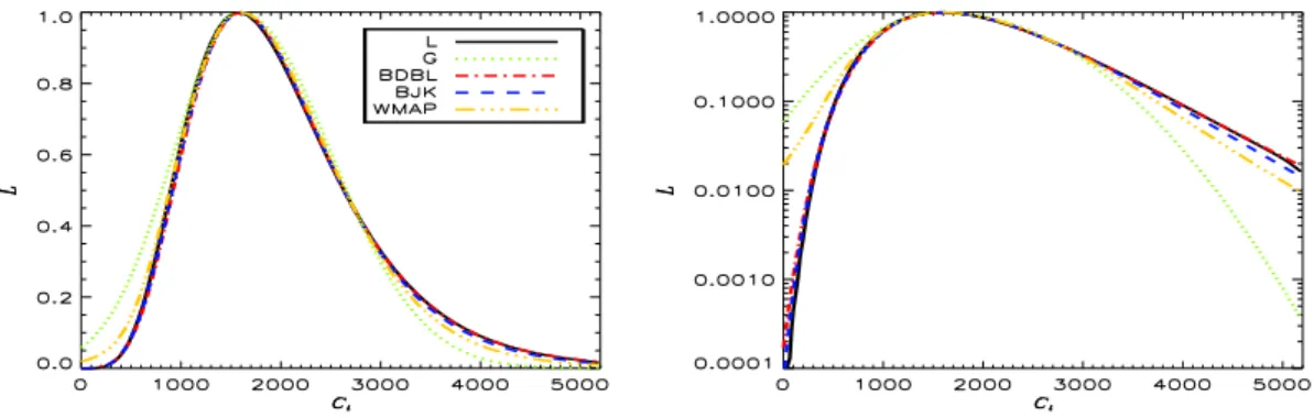
![Figure 1: Angular power spectrum estimates of the CMB anisotropies in September 2003 ([7, 8, 9, 10, 11, 12, 13, 14, 15])](https://thumb-eu.123doks.com/thumbv2/123doknet/2345153.34710/5.892.221.608.222.531/figure-angular-power-spectrum-estimates-cmb-anisotropies-september.webp)
Documents relatifs
It uses interferences in OFDM signal spectrum at the receiver (RX) in order to estimate the TDOA. This approach, allows to perform localization and data transmission simultaneously.
In contrast with classical techniques such as the EM algorithm, that define a precise likelihood function by averaging inside each imprecise observations, our approach presupposes
Key-words: Hidden Markov models, parameter estimation, particle filter, convolution kernels, conditional least squares estimate, maximum likelihood estimate9. (Résumé
The characterisation of the likelihood is completed in chapter 6 with the description of the Planck large scale data and the external datasets that are used in the estimation of
Subsequently, based on the derived aepdf expression, we present a technique to estimate the sparsity order of the wideband spectrum with compressive measurements using the
Then a new algorithm for frequency domain demodulation of spectral peaks is proposed that can be used to obtain an approxi- mate maximum likelihood estimate of the frequency slope,
In contrast with classical techniques such as the EM algorithm, that define a precise likelihood function by averaging inside each imprecise observations, our approach presupposes
Macovski, “Exact maximum likelihood parameter estimation of superimposed exponential signals in noise,” IEEE Transactions on Acoustics, Speech and Signal Processing, vol. Hua, “The
