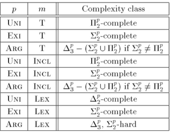
Non-monotonic reasoning: from complexity to algorithms
51
0
0
Texte intégral
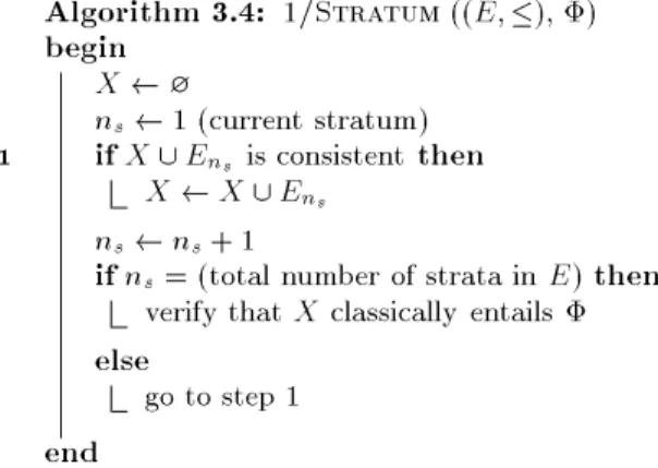
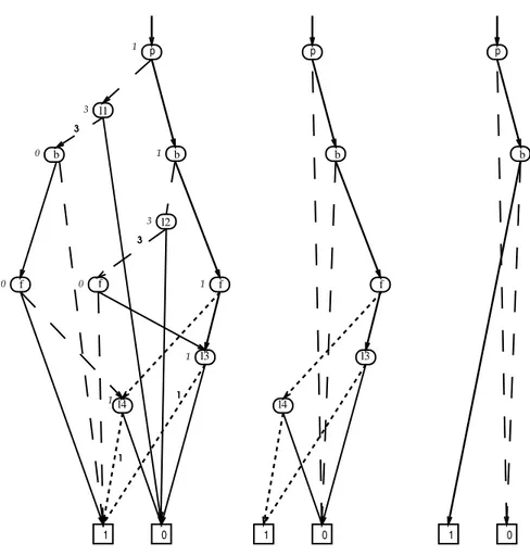
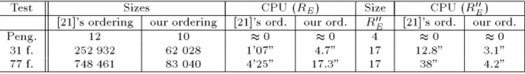
Figure

+4
Documents relatifs
