Deliverable D 2.1 – 6.1
Methodology proposal
01/08/2016
BRAIN-TRAINS
Transversal
assessment of new
intermodal strategies
BELGIAN RESEARCH ACTION THROUGH
INTERDISCIPLINARY NETWORKS
CONTENTS
CONTENTS ...2
INTRODUCTION ...3
DELIVERABLE 2.1: Methodology proposal for optimal corridor and hub development ...6
1. Identifying the managerial problem ...6
2. Modelling the problem using mathematical programming ...7
3. Computing the solutions ... 11
4. Translating the scenarios ... 12
REFERENCES... 13
DELIVERABLE 3.1: Methodology proposal for the macro-economic influence of rail freight transport ... 14
1. Problem identification: why measuring the macro-economic impact? ... 14
2. Methodology: Input-Output, multipliers and linkages ... 16
3. Risk analysis: data collection and validity of the results ... 23
4. Link with the scenarios: translation of tkm and a sensitivity analysis ... 24
REFERENCES... 26
DELIVERABLE 4.1: Methodology proposal for the sustainability impact of intermodality ... 28
1. Problem identification ... 29
2. Methodology ... 30
3. Link with the scenarios and perspectives ... 34
REFERENCES... 35
DELIVERABLE 5.1: Methodology proposal for the regulation policy ... 37
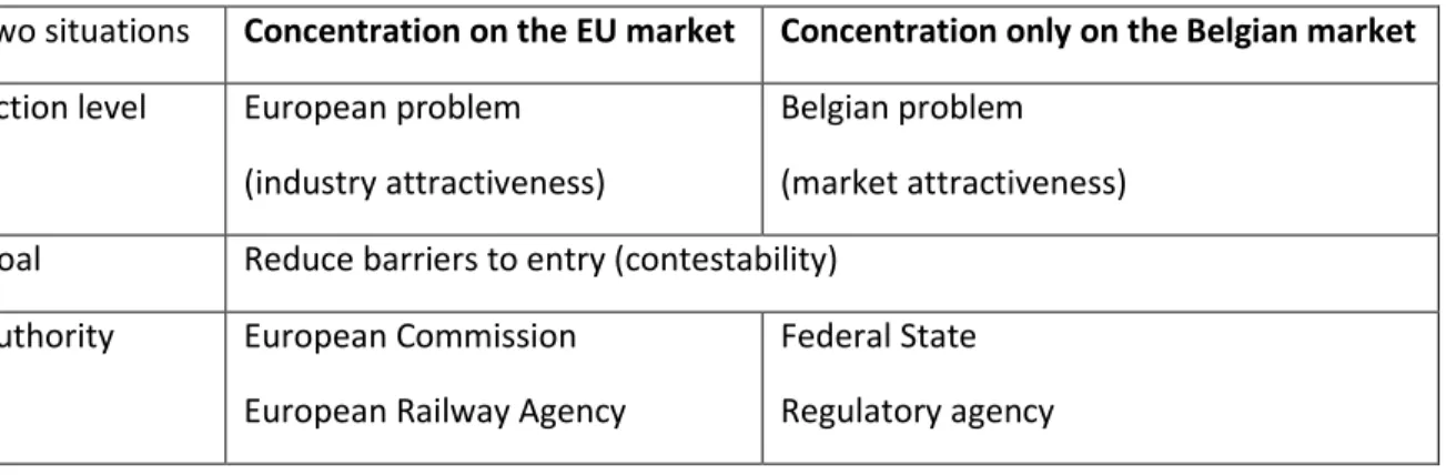
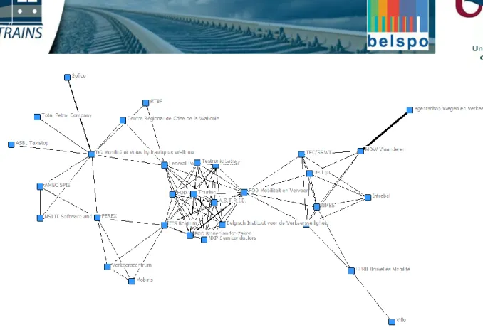
1. Problem identification : which market to regulate? ... 37
2. Data collection: limit of traditional databases ... 39
3. Methodology: tools for a market analysis ... 39
4. Link with the scenarios: a grid and tools to regulate the market ... 42
REFERENCES... 44
DELIVERABLE 6.1: Methodology proposal for an analysis on effective policy-making for a well-functioning intermodality ... 47
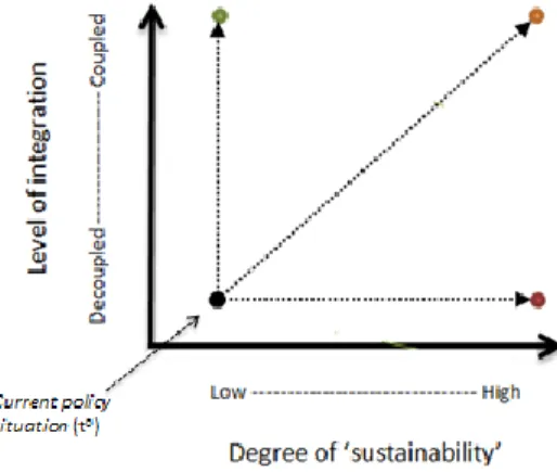
1. How to ensure ‘integration’? ... 47
2. Methodology ... 48
3. A glimpse at the final results ... 53
INTRODUCTION
The BRAIN-TRAINS project deals with the possible development of rail freight intermodality in Belgium. The main goal of the project is to develop a blue print establishing the detailed criteria and conditions for developing an innovative intermodal network in and through Belgium, as part of the Trans-European Transport Network and related to different market, society and policy-making challenges. The project develops an operational framework in which effective intermodal transport can be successfully established in Belgium, with attention to beneficial participation and commitment of all different stakeholders.
This analysis is built around five different main topics: (WP 2) The optimal corridor and hub-development. (WP 3) The macro-economic impact of intermodality. (WP 4) The sustainability impact of intermodality.
(WP 5) Effective market regulation for a well-functioning intermodality.
(WP 6) Effective governance and organization for a well-functioning intermodality. FIGURE 1:STRUCTURE OF THE BRAIN-TRAINS PROJECT
SOURCE:OWN COMPOSITION
Figure 1 is showing the process mapping for this transversal BRAIN-TRAINS project. The current document is providing more information on the developed methodologies for work package 2 to 6, indicated by the red frame
field. As such all five mentioned fields have developed a new or adapted methodology that will allow these quantifications to be made. The result of this methodology development process will be presented within this combined deliverable (D 2.1 – D 6.1). In a later phase of the project, the methodologies will be used on the earlier developed scenarios in order to create a model for each field that will allow to quantify and measure the impact of possible future developments and decisions on rail freight transport development in Belgium. The outcome of these field studies will then be combined in task 7, in order to develop the corresponding indicators, and to perform a final synthesis.
TABLE 1: WORK PACKAGE CHARACTERISTICS
SOURCE:OWN COMPOSITION
For the development of the different methodologies for the five corresponding work packages or tasks, a set of inputs, outputs and work package context assumptions has been made. The result of this internal discussion is shown in table 1 and is used as a starting point for each field to develop their corresponding methodology. In addition, this information will also be used as a guidance for the interpretation of future results from each work package. This table will also be of crucial importance when the output of all models will be combined in the last phase of the project, as mentioned in the section above.
All work packages will focus on rail freight transport in general, which includes also intermodal transport with rail as the main mode of transport for inland transportation. Work package 2 (WP 2) will also focus more on the specific intermodal component of rail transport within intermodal transport, indicating the optimal corridor and hub development for this specific part of rail transport in Belgium.
The main geographical scope of the research is Belgium, as previously defined. However, work package 2 and 5 will also take into account the European context, and more specifically the possible impact of the European rail corridors of which three are operating on Belgian territory. Other work packages will also take into account the European context, as rail transport is often an international business, but these effects will not be quantified within the corresponding models.
A last characteristic is the market perspective. Work package 3 to 6 will take into account an open market perspective, whereas work package 2 will built its model around a single operator perspective, in order to simplify the modelling, optimization and calculating techniques as described in chapter 2.1.
Input Output Rail in intermodal Transport
Rail Transport in general (incl. intermodal transport) Belgium Europe (rail corridors) Single operator perspective Multiple operator perspective (open market) Work Package 2 Optimal corridor and hub
development - emissions - taxes / subsidies - O-D matrix - operational cost (structure) - modal split - cost/emissions - frequencies - price - revenu + + + + + -Work Package 3 Macro-economic impact
- taxes and subsidies - VAT listings - supply and demand
tables (turnover) - added value - employment - multipliers - markov relations - + + - - + Work Package 4 Environmental impact - energy consumption - transport emissions - noise exposure
- life cycle assessment - + + - - +
Work Package 5 Regulatory impact - operators info - rail demand - optimal number of operators
- regulation best practices - + + + - +
Work Package 6 Public administration and
governance
- social network analysis - current level of
integration
- desired level of
TABLE 2:LINKS BETWEEN WORK PACKAGES
SOURCE:OWN COMPOSITION
Table 3 above is showing the different links that exist between the five work packages. The table should be interpreted from left to right. As such, there is not necessarily an equal mutual relationship between two work packages, as one work package can influence another on a high level, where the latter does not have any influence on the first work package. As for the symbols, ‘-‘ is indicating that there is no or a weak correlation between the two work packages. ‘+’ is representing a moderate to strong link and ‘++’ is showing a very high influence on the work package.
Work package 2 has a very strong link with all other work packages, except for work package 6 where a moderate correlation is observed. Especially the calculated modal split (output of WP 2) and the corresponding transported volumes by each mode will impact the scenarios and as such the input parameters for the other work packages. In addition, the change in prices and revenues will impact the input-output model of WP 3, emissions will be a mutual factor with WP 4 an the developed model of WP2 will be a tool to calculate certain findings in WP 5. Work package 3 is showing a moderate to strong impact on work packages 2, 5 and 6. Rail demand is a driving input factor for the input-output analysis in WP 3 and is therefore a common parameter with these work packages. In addition the studied Markov-chain relations between the different actors in WP 3 can be linked to the social network analysis performed in WP 6. There is only a limited direct correlation between the macro-economic impact (WP 3) and the environmental impact (WP 4)
The above mentioned factors also indicate a moderate to strong influence of work package 4 on work package 2, whereas work package 5 is influencing work package 3 and 6, and work package 6 is impacting on work package 3 and 5. Work Package 2 Optimal corridor and hub development Work Package 3 Macro-economic impact Work Package 4 Environmental impact Work Package 5 Regulatory impact Work Package 6 Public administration and governance Work Package 2 Optimal corridor and hub development ++ ++ ++ + Work Package 3 Macro-economic impact + - + + Work Package 4 Environmental impact ++ - - -Work Package 5 Regulatory impact - + - + Work Package 6 Public administration and governance - + - + Impact on
DELIVERABLE 2.1: Methodology proposal for optimal corridor and hub
development
CHRISTINE TAWFIK, MARTINE MOSTERT & SABINE LIMBOURG
QuantOM – UNIVERSITY OF LIEGE
Work package (WP) 2 aims at providing tools from the operations research domain, in order to highlight how effective intermodal rail transport is in Belgium. The objective of this package is also to give more insight on the decision-making process of the different stakeholders in the intermodal chain. The methods are based on the area of expertise of optimization, which aims at translating a managerial problem into a mathematical model that should be optimized. The main components of the methodology consist in:
1) Identifying the managerial problem.
2) Modelling the problem using mathematical programming. 3) Computing the solutions.
4) Translating the scenarios.
In this WP, two models are proposed to provide decision-making insights to the Belgian stakeholders of rail and intermodal rail transport. The first model stays at a strategic level and focuses on the network design of road and intermodal freight transport. The second model is at a tactical level and focuses on the service network design and pricing problems of intermodal rail transport.
The two models considered are developed in the following parts of the document.
1. IDENTIFYING THE MANAGERIAL PROBLEM
With the rising interest to stimulate intermodal transport, various topics provided interesting areas of research and investigation to the field of Operations Research. The first developed multi-modal network models that were able to handle intermodal flows appeared in the early 1990s (Caris et al., 2013). The most notable considered decision problems are intermodal freight location-allocation optimization problems, internalizing external costs, consolidation strategies and service network design.
1.1 Model 1
The managerial problem identified in this section is the location/allocation problem of intermodal terminals. When dealing with intermodal transport, some intermodal terminals are required on the route, in order to proceed to the transhipment of goods from one mode of transport to the other. Correctly locating intermodal terminals is of strategic importance in terms of intermodal competitiveness in relation to road (Mostert and Limbourg, 2016). Indeed, the main benefits of intermodal transport are generally obtained during the long-haul travel by the environment friendly mode of transport. However, if a terminal is wrongly located, it might increase the pre- and post-haulage distances by truck between the origin node and the first intermodal terminal, or between the second terminal and the destination node. If these drayage distances are too long, it can happen
that the long-haul travel by the environment friendly mode cannot compensate anymore for the disadvantages of the pre- and post-haulage travels by truck.
The model also tackles the allocation of flows between the different possible modes of transport. It allows determining the impact of specific policies on the flow repartition between intermodal and road transport. It can also show the flow transfers inside the intermodal market share, between rail and inland waterway (IWW), depending on the implemented initiatives.
1.2 Model 2
A particular aspect that closely affects intermodal transport competitiveness, and that is yet under-studied in the corresponding literature, is the determination of the right service tariffs, known as the pricing strategy (Bontekoning et al., 2004). Generally speaking, pricing strategies are distinguishable in the way they handle the interplay between profitability and competitiveness. A service price has to be high enough to cover the costs, and hence generate a profit, and low enough to remain attractive to the target customers. Bontekoning et al. (2004) identify two levels, at which the pricing strategy operates. The first level is that of the individual actor in the intermodal chain. Previous studies at this level were mainly concerned with calculating opportunity costs and providing educated pricing guidelines, mostly from the perspective of the network (main haul) and the drayage operators. The second level is that of the entire door-to-door chain. Service pricing decisions at this level are taken from the perspective of the service providers (carriers), while accounting for the potential competition and the target customers’ (shippers’) choices. As pointed out by the literature review in Tawfik and Limbourg (2015), there is a peculiar gap in the literature of solid optimization approaches tackling intermodal pricing problems that belong to the latter category. Nevertheless, their relative importance and relevance to the competitiveness of intermodal transport is acknowledged through the previously conducted SWOT analysis within the BRAIN-TRAINS project (Deliverable D1.1, D1.2).
We consider an approach that explicitly addresses intermodal service prices as decision variables within a numerical optimization problem. In particular, we highlight the non-trivial trade-off between the generated revenues through the collected tariffs and the cost expenses through the operated services; a service performance can be increased, and thus more customers attracted, at the expense of additional operating costs, and vice versa. The problem is tackled from the economic perspective of a single intermodal service provider, belonging to the tactical planning horizon and in the interest of profit maximization. Two main categories of joint decisions are examined: the service prices as received by the target clients and the service design reflected in their corresponding operating frequencies during a medium-term interval, typically one week.
2. MODELLING THE PROBLEM USING MATHEMATICAL PROGRAMMING
The second step of the methodology is to develop the mathematical formulation of the managerial problem. A mathematical optimization problem is composed of four main elements: parameters, variables, objective function and constraints. The input of the model consists of the different parameters, which take a fixed value. The output of the model consists in the variables, which are identified at the end of the optimization process. The model is structured according to two main parts: the objective function, that should be minimized or
maximized, and the different related constraints applicable to the problem under consideration. The generic structure of a general mathematical model is given by:
Minimize/Maximize Objective function Subject to: Constraint 1, Constraint 2, … Constraint n.
2.1 Model 1
The model developed in this section of WP2 allows optimizing two main kinds of objectives. The first one relates to economic aspects: trying to obtain the minimum total operational transportation costs on the road and intermodal networks. The second objective that can be optimized relates more to environmental concerns. This version of the modelling can indeed find the solution that minimizes the total amount of specific emitted air pollutants or external costs.
The main input parameters of the formulation are the distances (in km) between two nodes (each node representing a NUTS3 region) using a specific mode of transport (road, rail or IWW), the cargo-aggregated demand for one year between the nodes of the origin/destination matrix (in t), the costs/emissions/external costs values (in € or t of pollutants) for the transportation and transhipment of goods between modes, as well as the potential subsidies/taxes (in €/tkm) allocated to certain modes by public authorities. The output values consist of the location where to build additional terminals, the type of terminal to locate (rail or IWW), and the flow repartition (in tkm) between road, intermodal with rail, and intermodal with IWW transport.
The model is structured according to the following objective functions and constraints: Minimize either of the following:
Global operational costs. Air pollutant emissions. External costs.
Subject to:
A maximum of 𝑝 terminals can be located. Existing terminals should be open.
Demand should be satisfied. Flows should leave their origin.
Flows cannot go through a closed terminal.
Flows should be conserved between the intermodal terminals. Flows should be non-negative.
One characteristic of the model is that it can be used for solving one specific objective or for considering two potentially contradictory objectives at the same time (for instance, an economic versus an environmental objective). Under this configuration, a bi-objective model is thus solved, which leads to the generation of a set of Pareto-optimal pairs of solutions. The latter are solutions of the model, for which none of the objective functions can be improved, without worsening the value of the other one. Indeed, economic and environmental objectives may lead to different optimal solutions. Pareto equilibrium for these objectives is found when the optimal combination of economic-environmental objectives is reached, i.e. when it is not possible to reduce the obtained optimal value of costs, without increasing the value of the emitted pollutants/external costs. Different combinations of Pareto-optimal pairs can be found, depending on the level of economic or environmental optimality that should be achieved. The junction of all these combinations of economic-environmental objectives on a two-dimensional graph is called the Pareto frontier. The latter thus allows the decision-maker to make the choice inside a set of potentially optimal solutions, some focusing more on one objective, and others focusing more on the second one.
2.2 Model 2
A key issue in modelling the above proposed problem is how to represent the target shippers’ reasoning, and consequently, the demand volumes of the intermodal services in question. We notice an innate hierarchy in the problem’s definition due to the chronological order in the decision-making: first, the intermodal operator chooses his service pricing and design strategy, while, afterwards, the target shippers optimally react to those decisions by choosing (or not) the offered services.
In that sense, a certain optimization framework was proven adequate for similar hierarchical and non-cooperative decision schemes, yet largely overlooked in intermodal transport planning problems, namely: bilevel programming.
The concept is principally adapted from game theory, with the name of “Stackelberg games”. It depicts a game that involves two sequential layers of players: a leader and one or more follower(s). By definition, the leader has the privilege of making the first move in the game, while being able to anticipate the optimal reaction of the follower(s) to his chosen strategy. The solution (or the chosen strategy) is decided upon by working it backwards; the game is thus played from the point of view of the leader. Stackelberg games were first introduced into mathematical programming under the self-explanatory name of “mathematical programs with optimization problems in the constraints”, and became later known as “bilevel programs”.
The joint intermodal service pricing and design problem is constructed following a bilevel structure as follows:
Upper level (leader) Lower level (followers) Decision maker: Intermodal operator/service provider. Shipper firms.
Decisions: Services’ prices. Services’ frequencies.
Flows on leader’s (intermodal) itineraries. Flows on competition (= all-road itinerary).
An assumption that should remain unchanged throughout the model development is the ability for the competition, represented by trucking services, to accommodate all the demands of every shipper firm. It is thus ensured that the leader/intermodal operator is prevented from setting infinite tariff schedules on his services. It is equally important to assume that the competition shows no price or service quality change throughout the process.
Our formulation takes the initial form of a static path-based multi-commodity formulation, as introduced by Crainic (2000), while our bilevel model follows the main joint pricing and design structure as presented by Brotcorne et al. (2008).
2.3 Freight choice modelling
The general behavioural assumption is that shippers seek to minimize their total logistics costs, and thus increase their respective utility. In this context, utility is used in the sense of the received benefits or advantages from a purchased service according its corresponding value. To clarify, in standard passenger traffic, an individual decides on a certain mode of transportation (e.g.: car, public transportation, etc.) with respect to the realized benefits of this mode (i.e.: a weighted combination of the out-of-pocket expenses, transit time, safety, punctuality, etc.). Similarly, in freight transport, a mode/service choice is based on the realized utility. There is a sufficiently wide literature that considers a corresponding functional representation that goes beyond a trivial weighted sum of service attributes. Several individual items interact in complex ways in order to determine the total logistics costs, involving commodities’, shippers’ and shipments’ characteristics, in relation to level-of-service and mode attributes. An attempt to minimize a single cost element may result in an increase in the total costs.
We refer to Vieira (1992) for a generally acknowledged skeleton of logistics cost components: Transportation costs: freight chargers during transportation.
Mode-specific constants and variables: order and handling costs. Value of in-transit stocks: in-transit and inventory capital carrying costs.
Discount rate-related variables: loss, damage and unavailability of equipment costs.
Intangible service-related attributes: satisfaction with contract terms, perception of the effort to deal with the carrier and availability of Electronic Data Interchange (EDI) services.
Nevertheless, an application of a normative approach provided by cost models repetitively fails to coincide with the shippers’ actual choices. This is chiefly due to two reasons: the non-uniformity of the service perception among the shippers; and the lack of certain significant information for the cost calculation (e.g.: discount rate, cost per order and the number of days to collect a loss and damage claim).
The solution, as proposed by Ben-Akiva et al. (2013), is to combine discrete choice methods with the minimization of total logistics costs, in the same way that utility maximization is modelled for individuals’ choice behaviour in passenger traffic. The shippers’ modal selection can be specified in quantitative terms by employing a random utility model, where the choice model estimation is in fact an estimation of the missing cost variables information, together with the importance of the different cost components.
makers’ utility functions exactly, the utilities are treated by the analysts as random variables. What can be observed instead are the choices which depend on those utilities. Therefore, the event of choosing a certain alternative is considered stochastic with choice probability depending on the distributional assumption of the disturbance term in the utility function.
For the freight choice case, the utility of a certain mode 𝑖 for shipper 𝑛 is expressed as follows (Ben-Akiva et al., 2013):
𝑈𝑖𝑛= 𝜇(𝑙𝑜𝑔𝑖𝑠𝑡𝑖𝑐𝑠 𝑐𝑜𝑠𝑡𝑠𝑖𝑛) + 𝜀𝑖𝑛
Where:
𝜇: Negative scale parameter.
𝜀𝑖𝑛: Unobservable or random component.
The pool of data to be considered is based on a revealed preference (RP) approach that analyses actual choices in relation to the actual situation. In this exercise, prospective client firms of container transport are to be interviewed in a survey about time-average statistics for some of their specific origin-destination pairs, in order to reflect the effect of network characteristics uniquely. In particular, the following information is to be elicited through the survey:
Generic variables: size of the firm, annual sales, annual tonnage, availability of own fleet of vehicles, maximum acceptable delay, environment awareness and emissions’ penalization.
Mode-specific variables: corridor information, share among corridor shipments, shipment size, price of product shipped, freight rate, order unit cost, transit time, fraction of shipments arriving when wanted, fraction of shipments lost or damaged, fraction of time equipment being available, effort to deal with carrier and EDI availability.
To the extent of our knowledge, integrating a discrete choice methodology in the reaction of the followers within a bilevel pricing and design model is an innovative approach.
3. COMPUTING THE SOLUTIONS
Once the model formulation is developed, it should be translated into a programming language in order to be solved by a computer. The chosen programing language is Java and the model is solved through the use of a commercial solver developed by IBM: ILOG CPLEX 12.6. The formulation is solved on a personal portable computer (Windows 7, Dual-Core 2.5 GHz, 8 GB of RAM).
CPLEX, as a solver for such mathematical programs involving both discrete and continuous variables, applies state-of-the-art searching algorithms based on the idea of iteratively solving a sequence of the problem’s relaxation in order to provide bounds on the solution, known as: Branch-and-Bound. In the same context, a set of techniques are implemented at different stages to reach a tighter formulation and land an optimal solution more efficiently.
As for estimating the freight choice model within the second formulation, the open source freeware Biogeme will be used. Biogeme is designed for the maximum likelihood estimation of parametric models in general, with
4. TRANSLATING THE SCENARIOS
Once the optimal solution (single objective model) or the optimal pairs of solutions (bi-objective model) is generated, the last step of the methodology is to vary the different input parameters in order to assess the robustness of the modelling and also to evaluate the impact of different policies on the results.
Nevertheless, a set of basic assumptions will remain constant in all scenarios. In particular, within the service pricing and design model, we consider a fixed underlying physical network that comprises three modes of transportation: road, rail and inland waterways; as well as a set of terminals where the freight transhipment from one mode to another takes place. A service, in our notion, is defined by its origin, destination, transport mode and departure day of the week, while an intermodal itinerary is formed by at most three service legs. The network is assumed to be fully connected in terms of all-road/trucking services, making it feasible to accommodate the whole set of shippers’ demands.
Among the scenario parameters, we distinctly consider the following inputs:
Infrastructure and maintenance costs of the operating services, in terms of a fixed and variable component.
Road taxes, e.g.: Viapass. Subsidies.
Origin-destination matrix of flows over the network. Emission levels/external costs of pollutants.
The models compute in return the following outputs: Modal split, in terms of tkm.
Suggested intermodal service prices. Intermodal carrier’s profit.
Terminal locations.
Both models give the possibility to determine the impact of several initiatives on the listed outputs. The different scenarios developed in the deliverable 1.3 of the BRAIN-TRAINS project are implemented within this last part of the methodology. Indeed, in previous deliverables, the project proposed different important parameters to consider when dealing with intermodal and rail transport in Belgium. These parameters were retrieved out of a SWOT analysis, and selected for their relevance by a panel of experts, using the so-called Delphi method. Different values are assigned to each parameter, according to the scenario that is used (best-case, worst-case, middle-case). Our model will be tested according to these different scenario values and the results in terms of modal split (tkm), terminal location and type will be determined.
One objective of the BRAIN-TRAINS project is to provide interesting knowledge on rail and intermodal transport in Belgium in different areas of expertise. The most interesting issue in this framework is how the different work packages of this project can be linked together. The macro-economic, environmental, regulatory and public administration and governance domains all have strong links with the operational optimal corridor and hub development. To illustrate this connection, we develop here how the input/output of this model of WP2 are connected with the input/output of other WPs. The main common indicators between the model and the other WPs are the modal split and the calculated volumes in tkm. Indeed, this output of our model can be used as an
input of the model of the macro-economic impact package, in their input/output methodology. The amount of tkm on the Belgian network also serves as the basis of the computation of the global emissions for the environmental impact work package. The other way around, the amount of emissions per tkm calculated by WP4 can help in optimizing networks in terms of environmental impact. The calculated modal split and flow repartition will also influence the computation of the different scenarios for the regulatory issues of WP5. Finally, WP6 can also use modal split results in order to elaborate on the relationships linking the different actors of public administration, in the framework of intermodal and rail transport.
A further refinement of the computed outputs will be performed as part of the scenario calculations in next deliverables, provided the close links between the different WPs and the imaginable cyclic relationships, for the sake of verifying the modifications and validating the interactions between the WPs.
REFERENCES
Ben-Akiva, M., Meersman, H., Van De Voorde, E., 2013. Freight transport modelling. ISBN: 978-1781902851. Bontekoning, Y.M. , Macharis, C., Trip, J.J., 2004. Is a new applied transportation research field emerging? – A review of intermodal rail-truck freight transport literature. Transportation Research Part A 38, pp. 1-34.
Brotcorne, L., Labbé, M., Marcotte, P., Savard, G., 2008. Joint design and pricing on a network. Operations Research, vol. 56, no. 5, pp. 1104-1115.
Caris, A., Macharis, C., Janssens, G. K., 2013. Decision support in intermodal transport: a new research agenda. Computers in industry 64, pp. 105-112.
Crainic, T. G., 2000. Service network design in freight transportation. European Journal of Operational Research 122, pp. 272-288.
Mostert, M. & Limbourg (2016). External Costs as Competitiveness Factors for Freight Transport — A State of the Art. Transport Reviews, online.
Tawfik, C., Limbourg, S., 2015. Bilevel optimization in the context of intermodal pricing: state of art. Paper presented at the 18th Euro Working Group on Transportation, EWGT 2015, Delft, The Netherlands.
DELIVERABLE 3.1: Methodology proposal for the macro-economic influence of
rail freight transport
FRANK TROCH, THIERRY VANELSLANDER & CHRISTA SYS
TPR-UNIVERSITY OF ANTWERP
Work package (WP) 3 aims at providing tools from the macro-economic research domain, in order to measure the impact of rail transport on the Belgian economy. This research includes rail transport as a part of the intermodal chain. The SWOT analysis in deliverable 1.1 – 1.2 has shown that both economic growth and transport growth share a strong connection, impacting on one another (Hilferink, 2003). Although transport demand is a derived demand, and therefore usually following the economic growth and industrial production, changes within the transport sector and decisions impacting on transport in general do have an impact on the economic growth of a country as well (Konings et al., 2008; UNCTAD, 2014). As such it is important to understand and measure the relationship between rail transport and the national economy or macro-economic level.
Within this deliverable, the main components of the proposed methodology will be explained. An overview will be given according to four sequential steps:
1. Problem identification: why measuring the macro-economic impact? 2. Methodology: input-output, multipliers and linkages
3. Risk analysis: data collection and validity of the results
4. Link with the scenarios: translation of tkm and a sensitivity analysis
In this WP, the analysis will be built in three steps. First the framework of an input-output model is applied to the sector of rail operations and the multipliers for the national economy are calculated. In a second step, the connections between the different sectors of the national economy and the actors involved in rail transport are investigated through linkages between the rail freight sector and other industries of the national economy. Both steps are explained in section 2. Section 3 highlights possible problems and risks for the analysis of the current state. This current state will then be further analysed in a third step, by linking the scenarios from WP 1 to the obtained results. This will be discussed in section 4.
1. PROBLEM IDENTIFICATION: WHY MEASURING THE MACRO-ECONOMIC
IMPACT?
The SWOT analysis in WP 1 has shown the importance of high productivity, flexibility and a customer-oriented approach for rail transport and other related sectors, in order to obtain a competitive advantage and increase its attractiveness. Decisions and actions taken in the field of rail freight transport which aim at achieving these aspects also impact to a greater or lesser extent on the rest of the economy. As shown in figure 1, in order to quantify these effects, direct and indirect effects on the economic value should be taken into account, as well as direct and indirect effects on the strategic value (Kuipers et al., 2005; Coppens et al., 2005).
FIGURE 1–ECONOMIC IMPACT OF MEASURES DIRECTED TO FREIGHT TRANSPORT
SOURCE:OWN COMPOSITION BASED ON KUIPERS ET AL.(2005) AND COPPENS ET AL.(2005)
Economic value is expressed by the physical and monetary effects of policy measures. Direct effects of transport decisions and investments are often calculated by a classical cost-benefit analysis approach. However, Mouter et al. (2012) and Beukers et al. (2012) indicate the weakness of such approach due to the absence or underestimation of the indirect economic effects. In addition to the social costs and benefits, also indirect effects should be taken into account, which exist because the economic sectors are interrelated due to which changes in demand and supply in one sector ignite a ripple effect throughout the rest of the economy (Coppens et al. 2005).
Strategic value is often for many businesses and sectors a reason to remain active in a particular region or country. However, this effect is not always calculated in the direct and indirect economic value of transport. As such, it is important to also quantify the direct and indirect effects of the strategic significance of freight transport to the rest of the economy (Kuipers et al., 2005).
The goal of this WP is to develop a methodology to quantify both the economic and strategic value of rail freight transport. Coppens et al. (2007) performed a similar research for the economic impact of port activity, by applying a disaggregate analysis for the case of Antwerp. Within their study, the input-output technology is used to identify the multipliers capturing all direct and indirect economic effects, measured by the change of two macro-economic parameters: employment and added value. This information is then used to define the strategic value. This is done by using the Markov-chain to identify the relationships or linkages between port actors and the rest of the economy, and how these relationships can change under the influence of certain policy measures impacting the port and its environment.
In the next section, the input-output methodology will be explained, as well as the use of corresponding multipliers and the Markov-chain theory to identify strategic linkages. This will be done in the next section by means of a simplified example and the results obtained from the study of the port sector.
Economic
Value
•Direct •IndirectStrategic
Value
•Direct •IndirectEconomic
impact
Pol
icy
me
asur
es
2. METHODOLOGY: INPUT-OUTPUT, MULTIPLIERS AND LINKAGES
In order to capture the chain effect discussed in the previous section, the methodology of an input-output table is often used in similar studies. With this methodology, both the direct and indirect impact of modifications in the rail freight transport sector are captured by estimating the total effect on the national economy. However, whereas the port study by Coppens et al. (2007) used a regional input-output table, the study of economic impact of rail freight transport on the national economy requires using national input-output tables. The Federal Planning Office (2015) is publishing these national input-output tables every five years. The last version takes into account the input-output tables of 2010 and was published in December 2015.
2.1 General framework
The methodology of input-output analysis has been developed by the Russian economist Wissily Leontief (Miller & Blair, 2009). Table 1 gives a general overview of the structure of a national input-output table.
TABLE 1–STRUCTURE OF A NATIONAL INPUT-OUTPUT TABLE
1 2 … N X F C 1 c11 c12 … c1n x1 f1 c1 2 c21 c22 … c2n x2 f2 c2 … … … … … N cn1 cn2 … cnn xn fn cn M m1 m2 … mn mf VA va1 va2 … van C c1 c2 … cn
N = Number of industries in the economy Cij = Output of industry i delivered to industry j
Cn = total input / output of industry n
VA = Value added Mj = Import
Xi = Export
Fi = Final demand
SOURCE:OWN COMPOSITION BASED ON COPPENS (2006) AND COPPENS ET AL.(2007)
In a national input-output model, the economy is split into n industries. According to the NACE classifications, active companies are divided amongst these n industries (Coppens, 2007). The output of an industry i can be
delivered to a certain industry j, indicated by parameter Cij. Other possibilities are that the output of an industry
i is exported, indicated by parameter Xi, or is used by exogenous actors such as final consumption by families or
investments by the government. This is the final demand, indicated by parameter Fi. As such, the total output of
an industry i, indicated by parameter Ci, can be calculated according to formula (1):
𝑐𝑖 = ∑𝑛 𝑐𝑖𝑗
The same logic can be applied to obtain the purchases or input of each industry j (Coppens, 2006). The input of each industry i to industry j is added to the input or import bought from outside of the national economy,
indicated by parameter Mj. As the total input of a certain industry should be the same as the output of that
industry (ci = cj), the difference can be calculated as the added value that this industry is generating (Miller &
Blair, 2009). This is shown in formula (2) and (3):
𝑉𝐴𝑗= 𝑐𝑗− ∑𝑛 𝑐𝑖𝑗
𝑖=1 − 𝑚𝑖 (2)
𝑐𝑗 = ∑𝑛 𝑐𝑖𝑗
𝑖=1 + 𝑚𝑖+ 𝑉𝐴𝑗 (3)
2.2 Simplified example
How such an input-output table is calculated will be explained by using a simplified example based on Van Gastel (2015) and an illustration of input-output calculations by Miller and Blair (2009).
A first step is to collect the supply and demand tables from the national accounts. These tables are published every year by the National Bank of Belgium (NBB, 2015) and used every five years by the Federal Planning Office to calculate the national input-output table (Federal Planning Office, 2015). The supply and demand tables show the transactions between companies, indicating the structure of production costs, revenues generated from the production process, and transactions coming from import and export (NBB, 2015). The main difference between supply –and demand tables and an input-output table, is that the former identifies the relationship between products and industries, where the latter gives more insight in the mutual relationship between industries (Van Gastel, 2015).
Table 2 shows a simplified example of a possible supply table. Within this table, the output of each industry can be analysed.
For example, the chemicals industry is providing 100 units of PVC and 50 units of plastic. Cars are manufactured by the car manufacturing industry (200 units) and they are partially bought as an input from outside of the national economy (40). In this respect, import can be seen as an industry which is delivering an output of 40 units to the national economy.
TABLE 2–SIMPLIFIED SUPPLY TABLE
SOURCE:OWN COMPOSITION BASED ON VAN GASTEL (2015)
Chemicals Plastic Machines Car man. Energy prod. Import
PVC 100 0 0 0 0 0 Plastic 50 200 0 0 0 0 Machines 0 0 410 0 0 0 Energy 0 0 0 0 815 0 Cars 0 0 0 200 0 40 TOTAL 150 200 410 200 815 40
Table 3 shows a simplified example of a possible demand table. Within this table, the input of each industry can be analysed.
For example, the chemicals industry is using 5 units of PVC, 50 units of machines and 30 unit of energy. Cars are used by the car manufacturing industry (20 units) and they are partially sold to buyers outside of the national economy (190). In this respect, export can be seen as an industry which is buying an input of 190 units from the national economy. Cars are also used outside of the defined industries and export, resulting in a final demand by families and the government of 30 units.
TABLE 3–SIMPLIFIED DEMAND TABLE
SOURCE:OWN COMPOSITION BASED ON VAN GASTEL (2015)
It should be noticed that the sum of each corresponding row in table 2 and 3 would equal the same amount. This can be explained by the earlier statement that, on the condition that import, export, final demand and added value are included in the calculation, the total input of an industry should be the same as the total output of that industry (Miller & Blair, 2009). As such, the total amount of products used or exported should also equal the total amount produced or imported from this product.
For example, 240 cars are produced as an output (200 by the car manufacturing industry within the national economy and 40 are imported), while 240 cars are also used as an input (20 going to the car manufacturing industry, 190 are requested from outside the national economy and 30 are used by families and the government).
As a consequence, the added value for each industry can also be calculated. This is obtained by calculating the difference between what is needed for the total production of an industry and what is supplied as an output by this industry in return of these inputs. The added value for each industry is shown in table 3.
For example, the chemicals industry is producing and supplying 150 units (100 PVC + 50 plastic). In order to be able to produce these units, a total of 85 units is required by this industry (5 PVC + 50 machines + 30 energy). As such, the added value of the chemicals industry can be calculated as 65 (150 outputs – 85 inputs).
In a second step, the data of the demand table has to be corrected. The reason for this is that the obtained supply table is created based on the basic prices, or the actual product value based on the cost of production, where the demand table is calculated based on the commercial or market prices, including taxes, subsidies, transport margins and handling margins (Van Gastel, 2015). Indeed, companies can adapt the price of a product they are selling according to national laws, subsidies and their obtained profit margin (Coppens, 2006). Therefore, the price paid by an industry demanding a certain product is different from the actual product value. Within this
Chemicals Plastic Machines Car man. Energy prod. Export Final demand
PVC 5 20 0 0 0 75 0 Plastic 0 25 0 10 0 115 100 Machines 50 15 10 35 100 150 50 Energy 30 5 15 25 100 540 100 Cars 0 0 0 20 0 190 30 TOTAL 85 65 25 90 200 1070 280 Added Value 65 135 385 110 615 TOTAL 150 200 410 200 815 1070 280
example, it will be assumed that the demand table in table 3 is already adapted based on the remarks made in the previous paragraph.
In a third step, the actual merge of both tables can be executed. Thereby, the input-output table with a sector-sector comparison is obtained by calculating the ratio for each industry:
𝐼𝑛𝑝𝑢𝑡 − 𝑂𝑢𝑡𝑝𝑢𝑡 𝑐𝑜𝑒𝑓𝑓𝑖𝑐𝑖𝑒𝑛𝑡 𝑏𝑒𝑡𝑤𝑒𝑒𝑛 𝑠𝑒𝑐𝑡𝑜𝑟 𝐴 𝑎𝑛𝑑 𝐵 = ∑𝑛𝑖=1(𝑂𝑢𝑡𝑝𝑢𝑡 𝑜𝑓 𝑝𝑟𝑜𝑑𝑢𝑐𝑡 𝑖 𝑏𝑦 𝑠𝑒𝑐𝑡𝑜𝑟 𝐴 ∗
𝐼𝑛𝑝𝑢𝑡 𝑜𝑓 𝑝𝑟𝑜𝑑𝑢𝑐𝑡 𝑖 𝑏𝑦 𝑠𝑒𝑐𝑡𝑜𝑟 𝐵
𝑇𝑜𝑡𝑎𝑙 𝑖𝑛𝑝𝑢𝑡/𝑜𝑢𝑡𝑝𝑢𝑡 𝑝𝑟𝑜𝑑𝑢𝑐𝑡 𝑖) (4)
As such, the input – output relation between two sectors can be calculated by multiplying the output of each product of the first sector with the relative use of the concerned product by the second sector, and finally summarising the results for all products.
For example:
Industry A = Chemicals industry Industry B = Plastic industry
- For the product “PVC”: Output “PVC” by chemicals * (input “PVC” by plastic / Total I-O of “PVC”).
- For the product “Plastic”: Output “Plastic” by chemicals * (input “Plastic” by plastic / Total I/O of “PVC”).
- No other output is produced by the industry of chemicals.
Input-output relation between sector A and B =
100 * (20 / 100) + 50 * (25 / 250) + 0 * (15 / 410) + 0 * (5 / 815) + 0 * (0 / 240) = 20 + 5 + 0 + 0 + 0 = 25
TABLE 4–INPUT-OUTPUT TABLE
SOURCE:OWN COMPOSITION BASED ON VAN GASTEL (2015)
When the input-output coefficient between sectors is calculated using equation 4 for each possible relation between two industries, the input-output table is obtained as shown in table 4. The red circle shows the result of the example previously explained. It should be noted that the inversed relationship, between the plastic industry and the chemicals industry, results to 0. This can be explained by the information that the plastic
Chemicals Plastic Machines Car man. Energy prod. Export Final demand TOTAL
Chemicals 5 25 0 2 0 98 20 150 Plastic 0 20 0 8 0 92 80 200 Machines 50 15 10 35 100 150 50 410 Car. Man. 0 0 0 17 0 158 25 200 Energy prod. 30 5 15 25 100 540 100 815 Import 0 0 0 3 0 32 5 40 TOTAL 85 65 25 90 200 1070 280 Added Value 65 135 385 110 615 TOTAL 150 200 410 200 815 1070 280
the only relation between the plastics industry and the chemicals industry, is in the direction of chemicals providing inputs towards the plastic industry.
This also explains how the input-output table in table 4 can be read and interpreted. Reading it from left to right, the output relation between the row industry and the column industry can be analysed. The chemicals industry is indeed providing an output of 25 towards the plastic industry, whereas the plastic industry is not providing any output to the chemicals industry. Reading the table from top to bottom, the input relation is showing itself, by indicating what each column industry is using from a row industry. From the example, it is indeed clear that the plastic industry is using 25 inputs from the chemicals industry, whereas the chemicals industry is not using any input from the plastic industry.
2.3 Multipliers
An input-output table can be used to calculate technical coefficients for the national economy (Coppens, 2006; Miller & Blair, 2009). Then, these coefficients can be used to obtain multipliers that measure the impact of a change in input or output for one of the industries on the rest of the economy.
The Leontief multiplier measures the total effect on the output of the national economy by a change in final demand for one of the industries. It is expected that a change of one unit in final demand in industry i results in a total output change greater than the initial change of one unit. This is explained by the chain effect each change in final demand is invoking. In our example above, an increase in final demand from the plastic sector would not only result in a direct output increase for this sector. Instead, the plastic sector would require additional inputs from the sectors it is related to, in our example identified as the plastics industry, the chemicals industry, the machines industry and the energy industry. As such, the output from these industries would also increase, and in their turn these sectors would require additional inputs from the sectors they are related to. As such, a ripple effect would impact the total output of the national economy.
In order to calculate the Leontief multiplier for a sector, the technical input coefficients for the relationship between each industry needs to be obtained. This corresponds with the intermediate usage of products between industries. The following formulas can be used:
𝐴 = 𝐶 ∗ 𝑐−1 (5)
Where C is a matrix with all intermediate deliveries cij, as shown in table 1 and table 4, and c-1 is an inverted
diagonal matrix with the total inputs or outputs shown as ci. According to our example above, this would result
in the following matrices:
C = chemicals plastic machines car man. energy prod.
chemicals 5 25 0 2 0
plastic 0 20 0 8 0
machines 50 15 10 35 100
car man. 0 0 0 17 0
c-1 =
A =
These technical input coefficients can be interpreted as follows: for each euro output, the plastic industry needs 0.12 euro of purchases (input) from the chemicals industry, 0.10 euro of purchases from the own industry, … . The sum of the column for each industry is less than one, which can be explained by the absence of added value and import in this table (Coppens, 2006).
Based on the technical input coefficients from equation (5), the impact of a change in final demand on the national economy, taking into account the direct and indirect effects in the whole chain, can be calculated by:
𝐿 = (𝐼 − 𝐴)−1 (6)
With I a corresponding identity matrix and L being the (inverted) Leontief matrix, containing the technical output coefficients for the national economy. According to our example above, this would result in the follow matrix:
L =
The Leontief multiplier can be calculated by summarising all technical output coefficients of certain column industry. The result is called the Leontief multiplier for the corresponding industry and it can be interpreted as the total effect on the output of the national economy by a change of one unit in final demand for the concerned industry. In the example, each increase in final demand of the plastic industry by 1 euro, will result in a total output increase of 1.45 euro for the national economy of Belgium.
chemicals plastic machines car man. energy prod.
chemicals 1,03 0,14 0,00 0,02 0,00 plastic 0,00 1,11 0,00 0,05 0,00 machines 0,38 0,14 1,03 0,23 0,14 car man. 0,00 0,00 0,00 1,09 0,00 energy prod. 0,25 0,06 0,05 0,16 1,14 LEONTIEF 1,66 1,45 1,08 1,55 1,28
chemicals plastic machines car man. energy prod.
chemicals 1/150 0 0 0 0
plastic 0 1/200 0 0 0
machines 0 0 1/410 0 0
car man. 0 0 0 1/200 0
energy prod. 0 0 0 0 1/815
chemicals plastic machines car man. energy prod.
chemicals 0,03 0,12 0,00 0,01 0,00
plastic 0,00 0,10 0,00 0,04 0,00
machines 0,33 0,08 0,02 0,18 0,12
car man. 0,00 0,00 0,00 0,08 0,00
In addition, the Leontief multiplier can also be used to analyse the impact on the national employment by applying the same multiplier values to the corresponding employment data of each industry. In order to do this, the assumption that needs to be made is that the relation between output and employment remains unchanged when a shift in final demand is taking place (Coppens, 2006).
The Gosh multiplier is calculated similarly to the Leontief multiplier, but using the added value and import as an exogenous factor, instead of the final demand. This way, the Gosh multiplier is supply-driven, while the Leontief multiplier is demand-driven. The Gosh multiplier measures the total effect on the output of the national economy by an exogenous change in import or added value for one of the industries. A change of one unit in final demand in industry i results in a total output change expected to be greater than initial change of one unit (Coppens, 2006; Miller & Blair, 2009).
It should be noted that both models are using the assumption that the relations between the industries on one side, and final demand or import and added value on the other side are not changing when the demand or added value is increasing or decreasing (Coppens, 2006).
Finally, Oosterhaven and Stelder (2002) have applied a correction factor to the multipliers which makes it possible to multiply them with the total output without distortion. As such, the total share of generated effects on the total national economy of a whole industry can be calculated without any overestimations. This is the final version of the multipliers that has also been used in the study of economic impact from port activity (Coppens et al., 2007) and it is the multiplier that is proposed to be used in the analysis of this WP.
2.4 Interdependence or linkages of industries
In order to further analyse the relations between industries, three different indicators can be used based on the theory of the Markov-chain and its corresponding attributes: (i) Cai and Leung linkages, indicating the effect of an industry compared to its own output; (ii) decomposed linkages, indicating the effect of an industry compared to the output of the industry of concerned customers or suppliers and finally (iii) key sectors (Coppens, 2007). For the first two indicators, forward and backward linkages can be calculated. Forward linkages estimate the total effect of a certain industry on its customers. Backward linkages are showing the same relation, but for the suppliers of a certain industry. An overview of the formulas for these linkages is given in table 5. Within the formulas, lij refers to the Leontief technical output coefficients and gij refers to the Gosh technical output
coefficients, which are explained in section 2.3.
These linkages can be calculated between the industries that are taken into account in the input-output analysis. Due to data limitations, which will be explained in section three, the most important relations from the available national input-output analysis will be the relation between the rail freight industry and multiple customers and suppliers. Moreover, intermodal relations with land transport (road freight and pipeline transport), water transport (maritime freight and inland shipping), air transport and storage and supporting activities will be further investigated. Further analysis will need to make clear how national companies are distributed within the national input-output analysis over the different industries that are available, in order to be able to give a correct interpretation and understanding on the different industries involved.
TABLE 5–INPUT-OUTPUT INDICATORS REGARDING THE RELATIONS BETWEEN INDUSTRIES
SOURCE:CAI &LEUNG (2004),COPPENS ET AL.(2007)
3. RISK ANALYSIS: DATA COLLECTION AND VALIDITY OF THE RESULTS
In the previous section, it is indicated that a national input-output table is dividing the economy into a certain number of industries (Coppens, 2007). The Federal Planning Office is using 64 industry clusters for the Belgian national input-output table of 2010, based on the revised NACEBEL codes from NAI (Federal Planning Office, 2015). As it was mentioned before, a time delay for this kind of data of approximately 5 years has to be taken into account (Federal Planning Office, 2015). Corresponding to our research on rail freight transport, the lowest level of details publicly available in this national input-output table is classification number 49, including all companies active in the field of land transport and pipes transport. This includes both freight and passenger transport. As such, no conclusions can be drawn from this national input-output table for the rail freight industry. In addition, the national input-output table is also limited in terms of comparison of linkages and relations between the different industries, as this could only be done between the included 64 clusters. As a consequence, interesting relations such as the linkage between rail freight transport and shipping agents, freight forwarders, terminals and others transport actors cannot be analysed.
Taking this into account, the main difference between the port study of Coppens et al. (2007) and the current analysis of the rail freight sector and its impact on the Belgian economy should be explained. Whereas the port study is a disaggregate analysis, it is more focussed on the micro-economic level of the port industry. Only companies active within a geographically bound area, being the port of Antwerp, and a limited number of cluster industries, being the port actors, were taken into account. This set of companies was re-clustered in a new set of industries defined by the researchers. Applying the same bottom-up approach to the current analysis would require disaggregate micro-level data about all companies related to rail activities that are active in Belgium, and re-cluster them into an own defined set of industries linked to the rail freight sector. This would be the same work that the Federal Planning Office is doing every five years, although with a different set of industries. The
end result would be more of a micro-level analysis of the rail freight sector, without having a full picture of the macro-economic impact on the Belgian economy, which is the main objective of the current research.
Therefore, it should be accomplished to split the rail freight sector from the national classification number 49. In this way, the rail freight industry can be compared with the main national industries of the Belgian economy. According to the methodology described in section 2, this can be done by departing from the original supply – and demand tables for the Belgian economy, and re-clustering companies active in the rail freight industry into a new industry. As such, the rail freight industry is pulled from the land transport and pipes transport industry and can be analysed separately.
In order to obtain this result, a partnership has been started with the National Bank of Belgium and relations have been set-up with B Logistics, the incumbent Belgian rail operator who is still holding a market share of above 80% and therefore representing the biggest part of the rail freight industry in Belgium (Deville & Verduyn, 2012). The objective of this cooperation is to retrieve the necessary data to calculate the input-output analysis and the corresponding multipliers and linkages for the rail freight industry in Belgium.
A last remark with respect to the data is the validity of the results. The national input-output table and the data that will be collected during the research will take into account rail freight operators and their corresponding activities that are registered in Belgium and active on the Belgian geographical territory. As such, rail actions performed by international companies without establishment in Belgium will not appear in the data and will not be taken into account. Although these international operations also have a clear influence on the Belgian economy, the output of the current research should be interpreted as the macro-economic effect of national operations by national companies on the national economy.
4. LINK WITH THE SCENARIOS: TRANSLATION OF TKM AND A SENSITIVITY
ANALYSIS
The last published Leontief multiplier by the Federal Planning Office dates from May 2010, being calculated based on the input-output tables for Belgium for the year 2005. Although the input-output tables for Belgium for the year 2010 are also calculated and published in December 2015 (Federal Planning Office, 2015), the Leontief multipliers have not yet been calculated and analysed. As a first step towards the continuation of this research, this has been done as a start for further analysis and an exercise to learn the methodology described above. The results of this exercise can be found in table 6.
TABLE 6–LEONTIEF MULTIPLIERS FOR TRANSPORT SECTORS (2005 AND 2010 COMPARISON)
Industry (cluster) Multiplier 2005 Multiplier 2010
Land transport 1.73 1.66
Water transport 1.91 1.63
Air transport 1.82 1.72
This means that the industry of land transport has an effect of 1.73 on the national economy of 2005 and 1.66 in 2010. As a consequence, each euro increase in final demand in the industry of land transport results in an increase by 1.73 euro and 1.66 euro for the national Belgian economy, for 2005 and 2010 respectively. The decrease can be linked to the economic crisis that started in 2008, lowering the relative contribution of the transport sector to the macro-economic level of a country.
The results for the land transport industry can be compared with other transport industries, such as water transport and air transport. Where air transport provided a higher economic impact in both years, water transport faced a greater drop by 2010 compared to the other transport industries. The industry of storage and transport services is delivering a similar impact to the national economy compared to land transport. It should be emphasised that the land transport sector is mainly represented by road freight and public transport. As such, no direct conclusion can be taken for the rail freight industry.
When comparing to other industries in the Belgian economy, it can be stressed that the construction industry has the greatest impact on the national economy. With a multiplier of 2.14 in 2005 and 2.06 in 2010, each euro increase in final demand for the construction industry is resulting in more than an additional euro worth of indirect effects. The industry with the lowest effect on the national economy is education, with a multiplier of 1.12 in 2005 and 1.14 in 2010.
Looking at the strongest and weakest links for the industry of land transport, a first analysis shows that strongest link exists with the industry of storage and transport services, as well as legal services, leasing and the production industry of cokes and oil. The weakest link of land transport in terms of indirect output effects exists with the pharmaceutical industry and agriculture. It should again be mentioned that this analysis is based on aggregated data for the land transport sector as a whole, and therefore no conclusions can be drawn yet for the industry of rail freight transport.
After the calculation of the macro-economic impact of the rail freight industry on the national economy, the results of WP 3 will be linked to the scenarios developed in WP 1. Within this first WP, three different scenarios have been defined based on a SWOT that was performed for the rail freight sector. These scenarios are created by a set of parameters, indicating a worst-case evolution, a medium-case evolution and a best-case evolution for rail freight transport by 2030. As the model to measure the macro-economic impact is demand-driven, the parameter indicating the realised amount of ton-kilometre (tkm) will be of main importance for WP 3.
Based on the evolution of the amount of rail tkm in the three scenarios, the impact on the national economy can be estimated by applying this new demand to the collected data that was found for the analysis of the current state of the rail freight sector in terms of impact on the national economy. For the best-case scenario, an increase of rail freight demand by 133% is estimated. For the medium-case and worst-case scenario, this is respectively set to 64% and 10%. Taking into account the set growth parameters for the national economy in the corresponding scenarios, the data of the national supply –and demand tables and the data of the rail freight industry can be adapted accordingly, and the impact on the multipliers and linkages between the industries can be analysed.
By applying these scenarios to the set of data, in a first stage, the assumption is made that the relations between the sectors will remain unchanged. Therefore, a sensitivity analysis can be performed, in which different conditions are released and tested, to measure the influence on the outcome of the model. For example, one
REFERENCES
Beukers, E., Bertolini, L. & Brömmelstroet, M. (2012). Why cost benefit analysis is perceived as a problematic tool
for transport plans: a process perspective. Transportation Research Part A, 46 (1), pp. 68-78.
Cai, J., Leung, P. (2004). Linkage measures: a revisit and a suggested alternative. Economic systems research, 16 (1), pp. 63-85
Coppens, F. (2005). Indirect effects – A formal definition and degrees of dependency as an alternative to technical
coefficients. National Bank of Belgium Working Paper, 67.
Coppens, F. (2006). Input-outputanalyse : een mathematisch-economische handleiding. Eindwerk ingediend tot het behalen van de graad van licentiaat in de toegepaste economische wetenschappen. Faculteit van de Economische, Sociale en Politieke Wetenschappen en Solvay Business School, VUB, Brussel.
Coppens, F., Lagnaux, F., Meersman, H., Sellekaerts, N., Van de Voorde, E., Van Gastel, G., Vanelslander, T. and Verhetsel, A. (2007). Economic impact of port activity: a disaggregate analysis – the case of Antwerp. National Bank of Belgium Working Paper, 110.
Deville, X. & Verduyn, F. (2012). Implementation of EU legislation on rail liberalization in Belgium, France,
Germany and The Netherlands. National Bank of Belgium Working Paper, 221.
Federal Planning Office (2010). Input-outputtabellen 2005. Publication by FPB, publisher: Henri Bogaert, D/2010/7433/24, Brussels.
Federal Planning Office (2015). Input-outputtabellen 2010. Publication by FPB, publisher: Philippe Donnay, Brussels.
Hilferink, P. (2003). The correlation between freight transport and economic growth. 16th international
symposium on theory and practice in transport economics: 50 years of transport research: experience gained and major challenges ahead, Budapest, European Conference of Ministers of Transport.
Kuipers, B., Burgess, A., Manshanden, W. J. J., MTL, C. V., Muskens, A. C., Rustenburg, I. M. & Delft, P. (2005). De
economische betekenis van het goederenwegvervoer. TNO Rapport 2004-49. TNO Ruimte en Infrastructuur,
Delft.
Konings, R., Priemus, H. & Nijkamp, P. (2008). The future of intermodal freight transport: operations, design and
policy. Cheltenham, UK: Edward Elgar Publishing.
Miller R.E. & Blair P.D. (2009). Input-output analysis : foundation and extensions. Second edition. Cambridge University Press, The Edinburgh Building, Cambridge, United Kingdom.
Mouter, N., Annema, J. & Van Wee, B. (2012). Ranking the substantive problems in the dutch cost-benefit analysis
practice. Transportation research Part A: policy and practice, 49, pp. 241-255.
NBB (2015). Nationale rekeningen: gedetailleerde rekeningen en tabellen 2014. Nationale Bank van België, Brussel.
UNCTAD (2014). Review of maritime transport 2014. Publication UNCTAD/RMT/201, Geneva, United Nations. Van Gastel, G. (2015). Structural changes to the global economy. Presentation by Georges Van Gastel, Head of


![Risiko- & [und] Schutzfaktoren der psychischen Gesundheit humanitärer Einsatzhelfer : eine systematische Literaturübersicht](data:image/gif;base64,R0lGODlhAQABAIAAAP///wAAACH5BAEAAAAALAAAAAABAAEAAAICRAEAOw==)