Models with Missing Data by Canonical Transformation
N. GENGLER* and I. MISZTALt
"Fonds National Beige de la Recherche Scientifique, Unite d'Enseignement et de Recherche de Zootechnie, Faculte Universitaire des Sciences Agronomiques, B-5030 Gembloux, Belgium tDepartment of Animal SCiences, University of Illinois, Urbana 61801
ABSTRACT
An algorithm for approximation of reliability for multiple traits by multiple diagonalization was modi-fied to support missing data by weighting trans-formed contributions of records based on the pattern of missing data. The accuracy of approximation was assessed with simulated and field data by comparing approximate reliabilities with those from direct inver-sion. Simulated data had several levels of missing data and covariances between traits; correlations were close to those for linear type traits of dairy cattle. Field data were 1) dairy records for milk, fat, and protein yields with 26% of the observations for fat and protein removed and 2) beef records for birth weight, weaning weight, and mean gain after wean-ing with 43% of observations misswean-ing. These files also contained empty fixed effect classes. The algorithm worked best for simulated data, and, when covari-ances between traits decreased, proportion of missing traits decreased and the number of empty fixed classes decreased. For dairy data, improvement over single-trait reliability occurred only for traits with missing data; for beef data, little or no improvement occurred. The method is useful with multiple di-agonalization if the proportion of missing records or number of empty fixed effect classes or covariances between traits is moderate.
(Key words: reliability, multiple trait, animal model, missing data)
Abbreviationkey: PEV
=
prediction error variance.take much longer. If an identical model is used for each trait, a canonical transformation can save com-puting time and resources for multiple-trait models (11). Multiple diagonalization, which is an extended form of canonical transformation, accommodates more than one random effect (8, 11, 12). Recent develop-ments show that missing data for certain traits can be analyzed, as can different models per trait after combining single- and multiple-trait algorithms (4). Thus, multiple-trait models, canonical transforma-tion, and therefore also multiple diagonalization generally are applicable for prediction of breeding values for data files with missing observations. However, similar algorithms for computing approxi-mate measures of accuracy of prediction are not avail-able. For dairy cattle, the concept of reliability is mostly used to describe accuracy, which is defined as a linear function of the prediction error variance ( PEV) , expressed between 0 and 1.
A method to approximate reliabilities for single-trait models has been established (10, 13, 14). For multiple-trait models, methods have been developed to approximate reliabilities for a sire model (6) and for models using multiple diagonalization for data files with no missing observations (11). The objec-tives of this study were 1) to extend the latter method to accommodate missing data and 2) to demonstrate that different models per trait can be supported with multiple diagonalization without extra programming.
MATERIALS AND METHODS
Statistical Model
A multiple-trait linear model with t traits and records ordered within traits, where no observations are missing, is
INTRODUCTION
The solution for mixed models (7) associated with single-trait animal models and large data files now is possible and practical (11) using techniques that iterate on the data (15). For multiple-trait models, the same principles can be used, but computations
y
=
(It ® X) b + (It ® Z)p+ (It ® Z)a + e [1]
Received March 6, 1995.
Accepted October 18, 1995.
where y is the vector of observations, b is the vector of fixed effects, p is the vector of random permanent environmental effects, a is the vector of random
1996J Dairy Sci 79:317~28 317
Models with Missing Data by Canonical Transformation
N. GENGLER* and I. MISZTALt
"Fonds National Beige de la Recherche Scientifique, Unite d'Enseignement et de Recherche de Zootechnie, Faculte Universitaire des Sciences Agronomiques, B-5030 Gembloux, Belgium tDepartment of Animal SCiences, University of Illinois, Urbana 61801
ABSTRACT
An algorithm for approximation of reliability for multiple traits by multiple diagonalization was modi-fied to support missing data by weighting trans-formed contributions of records based on the pattern of missing data. The accuracy of approximation was assessed with simulated and field data by comparing approximate reliabilities with those from direct inver-sion. Simulated data had several levels of missing data and covariances between traits; correlations were close to those for linear type traits of dairy cattle. Field data were 1) dairy records for milk, fat, and protein yields with 26% of the observations for fat and protein removed and 2) beef records for birth weight, weaning weight, and mean gain after wean-ing with 43% of observations misswean-ing. These files also contained empty fixed effect classes. The algorithm worked best for simulated data, and, when covari-ances between traits decreased, proportion of missing traits decreased and the number of empty fixed classes decreased. For dairy data, improvement over single-trait reliability occurred only for traits with missing data; for beef data, little or no improvement occurred. The method is useful with multiple di-agonalization if the proportion of missing records or number of empty fixed effect classes or covariances between traits is moderate.
(Key words: reliability, multiple trait, animal model, missing data)
Abbreviationkey: PEV
=
prediction error variance.take much longer. If an identical model is used for each trait, a canonical transformation can save com-puting time and resources for multiple-trait models (11). Multiple diagonalization, which is an extended form of canonical transformation, accommodates more than one random effect (8, 11, 12). Recent develop-ments show that missing data for certain traits can be analyzed, as can different models per trait after combining single- and multiple-trait algorithms (4). Thus, multiple-trait models, canonical transforma-tion, and therefore also multiple diagonalization generally are applicable for prediction of breeding values for data files with missing observations. However, similar algorithms for computing approxi-mate measures of accuracy of prediction are not avail-able. For dairy cattle, the concept of reliability is mostly used to describe accuracy, which is defined as a linear function of the prediction error variance ( PEV) , expressed between 0 and 1.
A method to approximate reliabilities for single-trait models has been established (10, 13, 14). For multiple-trait models, methods have been developed to approximate reliabilities for a sire model (6) and for models using multiple diagonalization for data files with no missing observations (11). The objec-tives of this study were 1) to extend the latter method to accommodate missing data and 2) to demonstrate that different models per trait can be supported with multiple diagonalization without extra programming.
MATERIALS AND METHODS
Statistical Model
A multiple-trait linear model with t traits and records ordered within traits, where no observations are missing, is
INTRODUCTION
The solution for mixed models (7) associated with single-trait animal models and large data files now is possible and practical (11) using techniques that iterate on the data (15). For multiple-trait models, the same principles can be used, but computations
y
=
(It ® X) b + (It ® Z)p+ (It ® Z)a + e [1]
Received March 6, 1995.
Accepted October 18, 1995.
where y is the vector of observations, b is the vector of fixed effects, p is the vector of random permanent environmental effects, a is the vector of random
[
~:;~~
Z'YQJ [4] b=
(Q-1 @ I)bQ'P
=
(Q-1 @ In)PQ,
and il=
(Q-1 @ In)ilQ.A condition for the use of the multiple diagonaliza-tion is that no observadiagonaliza-tions for certain traits are missing. Ducrocq and Besbes (4) described a method that permits canonical transformation with missing data and the same incidence matrices for all traits. Their method is based on the replacement of a miss-ing observation with its expectation (3) using an expectation-maximization algorithm (9). Assume that a record of animalj contains two groups of traits, traits that are observed and traits that are missing.If Yj represents this record, then Yja is the part of the record containing the observed traits, and Yji3 is the part of the record with the missing traits. For itera-t ·IOn k'Yja~[kj
=
Yja' andwhere Ti
=
l!Oi, (Xi=
lIdj, and OJ and d j=
diagonal elements i of~and D, respectively. Original solutions can be obtained by backtransformation:[ X'X X'Z X'Z ] Z'X Z'Z + Til Z'Z Z'X Z'Z Z'Z + G:iA-1 [2] Y
=
( y'l Y2 Y~) " b=
(b~b~
b~)" p=
(p~ P2 p~)" a=
(a~ a2 a~)" and e=
(e~ e2 e~) ';where @ denotes a Kronecker product, and X and Z
contain incidence matrices. The (co)variance ma-trices of the random effects are defined as Varep)
=
P=
Po@ In,Var(a)=
G=
Go@A, and Var(e)=
R=
Ro@ I where Po, Go, and Ro are the (co)variance
ma-trices between traits, n is the number of animals, and A is the numerator relationship matrix. The mixed model equations can be expressed as
animal effects, and e is the vector of random residual effects:
Multiple Random Effects and Missing Data
Let L be the Cholesky factor ofRo (i.e., Ro
=
LL'). Multiple diagonalization ofthe (co)variance matrices Po, Go, and R o is possible ifa matrix B exists that satisfies the following three equationswhich can be rewritten as
i\o[k] _
x.
b~[kl + p~[kj + ark] + e~J['~]orji3 - -'"ji3 ji3 ji3 ji3 I' [5]
where D and ~ are diagonal matrices, and I is an identity matrix. Such a matrixB exists if one of the three matrices can be expressed as a linear function of the other two. In other cases, a good approximation often exists (5). If [3] is true, the transformation matrix can be defined as Q
=
(LB)-1, with QPoQ'=
.6., QGoQ'=
D, and QRoQ'=
I. Then Y is transformed to YQ by YQ=
(Q ® In)y.The mixed model Equations [2] associated with the original Model [1] can be simplified and split into t independent single-trait mixed model equations:
L-1Ro( L-1)' L-1Go( L-1)' L-1Po( L-1)'
=
BIB',=
BDB', and=
B.6.B'; [3)wher~ Xji3 is the submatrix ofX that associates Yj/3 and bW All the terms on the right side of the equa-tion are obtained as soluequa-tions from iteraequa-tion k, except for the residuals for missing observations, which are estimated to be the regression of those residuals on the current estimates of the residuals for observed traits. These calculations represent the expectation step of the expectation-maximization algorithm.
At iteration k +1,a missing observation is replaced by its expectation, and new solutions for b, p, and a are obtained (the maximization step). Ducrocq and Besbes (4) proposed a method to avoid backtransfor-mation that simplified computations.
Different Models per Trait
Ducrocq and Besbes (4) also showed that canoni-cal transformation can support different sets of fixed
Journal of Dairy Science Vol. 79, No.2, 1996
[
~:;~~
Z'YQJ [4] b=
(Q-1 @ I)bQ'P
=
(Q-1 @ In)PQ,
and il=
(Q-1 @ In)ilQ.A condition for the use of the multiple diagonaliza-tion is that no observadiagonaliza-tions for certain traits are missing. Ducrocq and Besbes (4) described a method that permits canonical transformation with missing data and the same incidence matrices for all traits. Their method is based on the replacement of a miss-ing observation with its expectation (3) using an expectation-maximization algorithm (9). Assume that a record of animalj contains two groups of traits, traits that are observed and traits that are missing.If Yj represents this record, then Yja is the part of the record containing the observed traits, and Yji3 is the part of the record with the missing traits. For itera-t ·IOn k'Yja~[kj
=
Yja' andwhere Ti
=
l!Oi, (Xi=
lIdj, and OJ and d j=
diagonal elements i of~and D, respectively. Original solutions can be obtained by backtransformation:[ X'X X'Z X'Z ] Z'X Z'Z + Til Z'Z Z'X Z'Z Z'Z + G:iA-1 [2] Y
=
( y'l Y2 Y~) " b=
(b~b~
b~)" p=
(p~ P2 p~)" a=
(a~ a2 a~)" and e=
(e~ e2 e~) ';where @ denotes a Kronecker product, and X and Z
contain incidence matrices. The (co)variance ma-trices of the random effects are defined as Varep)
=
P=
Po@ In,Var(a)=
G=
Go@A, and Var(e)=
R=
Ro@ I where Po, Go, and Ro are the (co)variance
ma-trices between traits, n is the number of animals, and A is the numerator relationship matrix. The mixed model equations can be expressed as
animal effects, and e is the vector of random residual effects:
Multiple Random Effects and Missing Data
Let L be the Cholesky factor ofRo (i.e., Ro
=
LL'). Multiple diagonalization ofthe (co)variance matrices Po, Go, and R o is possible ifa matrix B exists that satisfies the following three equationswhich can be rewritten as
i\o[k] _
x.
b~[kl + p~[kj + ark] + e~J['~]orji3 - -'"ji3 ji3 ji3 ji3 I' [5]
where D and ~ are diagonal matrices, and I is an identity matrix. Such a matrixB exists if one of the three matrices can be expressed as a linear function of the other two. In other cases, a good approximation often exists (5). If [3] is true, the transformation matrix can be defined as Q
=
(LB)-1, with QPoQ'=
.6., QGoQ'=
D, and QRoQ'=
I. Then Y is transformed to YQ by YQ=
(Q ® In)y.The mixed model Equations [2] associated with the original Model [1] can be simplified and split into t independent single-trait mixed model equations:
L-1Ro( L-1)' L-1Go( L-1)' L-1Po( L-1)'
=
BIB',=
BDB', and=
B.6.B'; [3)wher~ Xji3 is the submatrix ofX that associates Yj/3 and bW All the terms on the right side of the equa-tion are obtained as soluequa-tions from iteraequa-tion k, except for the residuals for missing observations, which are estimated to be the regression of those residuals on the current estimates of the residuals for observed traits. These calculations represent the expectation step of the expectation-maximization algorithm.
At iteration k +1,a missing observation is replaced by its expectation, and new solutions for b, p, and a are obtained (the maximization step). Ducrocq and Besbes (4) proposed a method to avoid backtransfor-mation that simplified computations.
Different Models per Trait
Ducrocq and Besbes (4) also showed that canoni-cal transformation can support different sets of fixed
effects per model by computing these effects as in a regular multiple-trait procedure and then transform-ing data adjusted for the fixed effects. Although this method extended canonical transformation to general models, computer programming had to include a procedure to solve multiple-trait models and, there-fore, was complicated. The same result can be accom-plished for multiple diagonalization and, therefore, also for canonical transformation without additional programming by 1) declaring all fixed effects for each trait, 2) splitting each record into multiple records such that each new record contains the same combi-nation of fixed effects, and 3) assigning values of unneeded fixed effects to a "dummy" level for each new record. If every trait has a different model, each new observation contains one known trait with all remaining traits unknown. This approach results in increased storage requirements for data files unless splitting the records is incorporated into the iteration program.
Numerical example. Consider a joint analysis for
production traits and final score, in which milk, fat, and protein records are distributed in fixed herd-year-season classes, and final score records are grouped according to fixed herd-year-month-classification classes and are also affected by the classifier effect. Consider the following records for three cows A, B, and C:
Approximation of Reliability
Let WQi be the diagonal matrix of PEV of the t transformed traits for animal j. Following the method of Misztal et a1. (11), if Wj is the matrix of PEV for the original traits, then
The PEV for the transformed traits can be obtained using the method proposed by Misztal and Wiggans (13): WQij
=
lI(aj + bij), where wQjj is PEV of trans-formed trait i of animal j, ai=
lIdj, and bjj is the information on animal j expressed as effective records (11, 13). This information is assumed to be a sum of contributions from own records (fjj) and from im-mediate relatives (parent or progeny) of animal k (g ijk):where fij and gjjk were derived as in Misztal and Wiggans (13). For a repeatability model with one important fixed effect, reduction of information be-cause of fitting the permanent environmental effect is reflected by
where Tj is a variance ratio for permanent environ-ment for trait i, and Zij is the numbers of records adjusted to reflect the reduction of information be-cause of fitting the fixed effect:
where nl is the number of records in fixed effects subclass 1when cow j has a record.
The contribution from pedigree is obtained by an iterative procedure (13). If no observations are miss-ing for the original traits, the contributions fjj differ only between transformed traits because of different permanent environmental variances. If some observa-tions are missing, bjj is overestimated, and, conse-quently, WQij is underestimated. Contributions gjjk are affected indirectly because they are functions of bij'
To examine the reduction of bjj because of missing data, assume that after multiple diagonalization, the left side of the coefficient matrix of Equation [4] can be approximated:
Herd· year-Herd· month·
year· classif· Final
Cow season ication Classifier Milk Fat Protein score
A 1 1 1 6000 200 175 78
B 2 2 1 7000 225 200 80
C 2 3 2 8000 250 225 82
They can be rewritten using the algorithm just described:
Main
fixed Final
Cow effect Classifier Milk Fat Protein Bcore
A 1 0 6000 200 175 M B 2 0 7000 225 200 M C 2 D 8000 250 225 M A 1 1 M M M 78 B 2 1 M M M 80 C 3 2 M M M 82
where the main fixed effect represents herd-year-season for yield traits or herd-year-month-classification for final score, M is the code for missing values, and D is the code for a dummy level, which in this case is 1.
Zjj
= I/l -
lInl) , 1[7]
[8]
effects per model by computing these effects as in a regular multiple-trait procedure and then transform-ing data adjusted for the fixed effects. Although this method extended canonical transformation to general models, computer programming had to include a procedure to solve multiple-trait models and, there-fore, was complicated. The same result can be accom-plished for multiple diagonalization and, therefore, also for canonical transformation without additional programming by 1) declaring all fixed effects for each trait, 2) splitting each record into multiple records such that each new record contains the same combi-nation of fixed effects, and 3) assigning values of unneeded fixed effects to a "dummy" level for each new record. If every trait has a different model, each new observation contains one known trait with all remaining traits unknown. This approach results in increased storage requirements for data files unless splitting the records is incorporated into the iteration program.
Numerical example. Consider a joint analysis for
production traits and final score, in which milk, fat, and protein records are distributed in fixed herd-year-season classes, and final score records are grouped according to fixed herd-year-month-classification classes and are also affected by the classifier effect. Consider the following records for three cows A, B, and C:
Approximation of Reliability
Let WQi be the diagonal matrix of PEV of the t transformed traits for animal j. Following the method of Misztal et a1. (11), if Wj is the matrix of PEV for the original traits, then
The PEV for the transformed traits can be obtained using the method proposed by Misztal and Wiggans (13): WQij
=
lI(aj + bij), where wQjj is PEV of trans-formed trait i of animal j, ai=
lIdj, and bjj is the information on animal j expressed as effective records (11, 13). This information is assumed to be a sum of contributions from own records (fjj) and from im-mediate relatives (parent or progeny) of animal k (g ijk):where fij and gjjk were derived as in Misztal and Wiggans (13). For a repeatability model with one important fixed effect, reduction of information be-cause of fitting the permanent environmental effect is reflected by
where Tj is a variance ratio for permanent environ-ment for trait i, and Zij is the numbers of records adjusted to reflect the reduction of information be-cause of fitting the fixed effect:
where nl is the number of records in fixed effects subclass 1when cow j has a record.
The contribution from pedigree is obtained by an iterative procedure (13). If no observations are miss-ing for the original traits, the contributions fjj differ only between transformed traits because of different permanent environmental variances. If some observa-tions are missing, bjj is overestimated, and, conse-quently, WQij is underestimated. Contributions gjjk are affected indirectly because they are functions of bij'
To examine the reduction of bjj because of missing data, assume that after multiple diagonalization, the left side of the coefficient matrix of Equation [4] can be approximated:
Herd· year-Herd· month·
year· classif· Final
Cow season ication Classifier Milk Fat Protein score
A 1 1 1 6000 200 175 78
B 2 2 1 7000 225 200 80
C 2 3 2 8000 250 225 82
They can be rewritten using the algorithm just described:
Main
fixed Final
Cow effect Classifier Milk Fat Protein Bcore
A 1 0 6000 200 175 M B 2 0 7000 225 200 M C 2 D 8000 250 225 M A 1 1 M M M 78 B 2 1 M M M 80 C 3 2 M M M 82
where the main fixed effect represents herd-year-season for yield traits or herd-year-month-classification for final score, M is the code for missing values, and D is the code for a dummy level, which in this case is 1.
Zjj
= I/l -
lInl) , 1[7]
* _
[R~l
0]
R· - ,
J 0 0
where Hid is a diagonal matrix of weights that reflect the contributions of observations. New formulas for the contribution of records are derived by analyzing submatrices of Equation [9].
The fixed effect and animal equations for trait i of animal j with a record in fixed effects subclass 1are
and R~l is the inverse of the part of Ro that is associated with nonmissing traits. Rj*is also a partic-ular generalized inverse of
Ro,
the residual (co)variance matrix of original traits with zeros in rows and columns corresponding to missing data. On the transformed scale, we can computen1 'Yijl 'Yijl
'Yijl
L
'Yijl + Ti L'Yijl1 1
'Yijl
L
'Yijl L'Yijl +ar ..
J1 1 [13] * By isolating Wj ' where
r
= 'Ytjand 'Yij are contributions from one record, reduced to reflect lack of contributions from missing data. Exact PEV on the original scale (WI) is
[14J
In Equation [15], an approximate diagonalization of W; is performed, and the resulting off-diagonals are discarded. With all traits recorded, the equation is exact because [diag(QWjQ')J-1 - D-1
=
It>or 'Yij=
1. If some traits are missing, QWj*Q' has off-diagonal elements, and Equation [15] is an approximation only. Equation [15J also gives exact results ( 'Yij = 0 if trait i is missing, and 'Yij = 1 if i is not missing) if (co)variances between traits are 0, which is equiva-lent to the single-trait model. As a matter of fact, given Equation [15], the approximation improves if* '
off-diagonals of QWj Q are small.
For computing PEV of individuals, different possi-bilities exist to approximate G. They can be based on equating complete formulas or only diagonals on either the original or transformed scale. The three most obvious possibilities are based on an approxi-mate diagonalization ofRj*, on equating diagonals of Equations [12] and [14], or on equating diagonals of Equations [11] and [13J. Preliminary tests using these and other possibilities were done and showed the superiority of the last approach, which can be rewrit-ten as [10] [l1J
o
y. IJo
z" = ~{'Y"I(l - I'"l/n'l) } IJ "'" IJ I J ' Iwhere 'Yijl represents a reduction in reliability because of missing data. Once 'YijI is approximated, approxi-mate reliabilities can be calculated.
Ifa coefficient matrix for only one animal and one observation is considered and all other fixed and per-manent environmental effects are ignored, then PEV on the transformed scale is assumed to be
where 'Yijl is the part of transformed trait i with observations present, and n; is the sum of 'Yijl in fixed effect subclass 1. After the sequential absorption of the equations for fixed effect subclasses and perma-nent environment into the animal equation, Equation
[7] does not change, and Equation [8] becomes
where R; is in the case of ordered traits (present before missing):
* * -1 -1
Wj = [Rj + Go] , [12] Algorithm
The algorithm to calculate the approximate relia-bilities for a large-scale multitrait animal model with missing data follows:
Journal of Dairy Science Vol. 79, No.2, 1996
* _
[R~l
0]
R· - ,
J 0 0
where Hid is a diagonal matrix of weights that reflect the contributions of observations. New formulas for the contribution of records are derived by analyzing submatrices of Equation [9].
The fixed effect and animal equations for trait i of animal j with a record in fixed effects subclass 1are
and R~l is the inverse of the part of Ro that is associated with nonmissing traits. Rj*is also a partic-ular generalized inverse of
Ro,
the residual (co)variance matrix of original traits with zeros in rows and columns corresponding to missing data. On the transformed scale, we can computen1 'Yijl 'Yijl
'Yijl
L
'Yijl + Ti L'Yijl1 1
'Yijl
L
'Yijl L'Yijl +ar ..
J1 1 [13] * By isolating Wj ' where
r
= 'Ytjand 'Yij are contributions from one record, reduced to reflect lack of contributions from missing data. Exact PEV on the original scale (WI) is
[14J
In Equation [15], an approximate diagonalization of W; is performed, and the resulting off-diagonals are discarded. With all traits recorded, the equation is exact because [diag(QWjQ')J-1 - D-1
=
It>or 'Yij=
1. If some traits are missing, QWj*Q' has off-diagonal elements, and Equation [15] is an approximation only. Equation [15J also gives exact results ( 'Yij = 0 if trait i is missing, and 'Yij = 1 if i is not missing) if (co)variances between traits are 0, which is equiva-lent to the single-trait model. As a matter of fact, given Equation [15], the approximation improves if* '
off-diagonals of QWj Q are small.
For computing PEV of individuals, different possi-bilities exist to approximate G. They can be based on equating complete formulas or only diagonals on either the original or transformed scale. The three most obvious possibilities are based on an approxi-mate diagonalization ofRj*, on equating diagonals of Equations [12] and [14], or on equating diagonals of Equations [11] and [13J. Preliminary tests using these and other possibilities were done and showed the superiority of the last approach, which can be rewrit-ten as [10] [l1J
o
y. IJo
z" = ~{'Y"I(l - I'"l/n'l) } IJ "'" IJ I J ' Iwhere 'Yijl represents a reduction in reliability because of missing data. Once 'YijI is approximated, approxi-mate reliabilities can be calculated.
Ifa coefficient matrix for only one animal and one observation is considered and all other fixed and per-manent environmental effects are ignored, then PEV on the transformed scale is assumed to be
where 'Yijl is the part of transformed trait i with observations present, and n; is the sum of 'Yijl in fixed effect subclass 1. After the sequential absorption of the equations for fixed effect subclasses and perma-nent environment into the animal equation, Equation
[7] does not change, and Equation [8] becomes
where R; is in the case of ordered traits (present before missing):
* * -1 -1
Wj = [Rj + Go] , [12] Algorithm
The algorithm to calculate the approximate relia-bilities for a large-scale multitrait animal model with missing data follows:
1. For every observation, compute 'Yij as in Equa-tion [15].
2. For every animal, compute adjustments for fixed effects as in Equation [10], and then adjust for permanent environmental effect as in Equation [71.
3. After calculating fij, the adjustment for effect of permanent environment, compute the single-trait PEV algorithm of Misztal and Wiggans ( 13) for each of t traits.
4. Backtransform PEV as in Equation [6].
5. Compute reliabilities for every animal and origi-nal trait as 1 - (wi/(j~), where wij is the PEV for original trait i and animal j and(j~ is the genetic variance of original trait i.
Comparison of Rellablllties Approximated with and Without Correction for Missing Data
Reliabilities were calculated for simulated and field data. (Co)variance matrices used were checked to be positive definite.
Simulated data. Data were simulated for 900 cows with records having 400 ancestors. All cows had a minimum of one record with a random number of additional records with up to 10 records for one animal. A total of 3000 records was grouped in 100 classes for fixed effects. The design was unbalanced, and the classes for fixed effects contained from 17 to 46 observations. Records were distributed randomly among fixed effect classes.
For the first simulated data file (F1), random effects included additive genetic, permanent environ-mental, and residual effects with respective (co )variances: [ 1000 500 -900] Po
=
500 2000 -100 , -900 -100 2000 [ 4000 500 700] Go=
500 3000 -1000 700 -1000 2000 and [ 2000 1000 -1800] Ro=
1000 4000 -200. -1800 -200 4000These genetic parameters correspond to correlations reported by Misztal et al. (12) for type traits. Three other data files (F2, F3, and F4) were simulated with
identical variances but with covariances of 0.1, 0.5, and 1.4 times the covariances of F1, respectively. These four data files were examined with various percentages (0, 11, or 33%) of data considered miss-ing to determine whether correlations decreased as covariances increased. Observations to be considered missing were randomly chosen, but three missing observations for one record were avoided.
Dairy field data. Data for dairy cattle were ob-tained from A. Toussaint, and A. De Bast (]~levage Informatique, Ciney, Belgium) and included 5809 305·d records for milk, fat, and protein from 500 cows chosen randomly and their 3108 contemporaries in 614 herd-year-seasons. The number of animals to-taled 6072 with ancestors included. Variance and covariance components, expressed in square kilo· grams, were obtained from another study with simi-lar but more data (P. Coenraets and N. Gengler, 1994, personal communication): [ 126, 102 4508 3538] Po
=
4508 271 145 3538 145 115 [ 153,767 4925 3890l Go = 4925 347 1561, 3890 156 123J and [ 484,291 19,429 15,098] Ro=
19,429 973 641. 15,098 641 510Data for protein and fat were considered to be missing for 26% of records, with 9% of the missing observations concentrated in the 58 most recent herd-year-seasons and the other 17% dispersed randomly among other records. The purpose of eliminating some data was to provide a realistic situation for Belgium and the US in which information on protein or on fat and protein was missing.
Beeffield data. Data for beef cattle were obtained from R. E. Golden (1994, Colorado State University, Fort Collins) and included 7270 records for birth weight (7270 observations), weaning weight (7270 observations), and postweaning gain (4150 observa-tions) with a total of 7864 cattle. The model included fixed management effects, which were assumed to be common to all traits, and random animal effects, but not permanent environmental or maternal effects. (Co)variance, expressed as square kilograms, was based on information from B. Klei (Cornell Univer-1. For every observation, compute 'Yij as in
Equa-tion [15].
2. For every animal, compute adjustments for fixed effects as in Equation [10], and then adjust for permanent environmental effect as in Equation [71.
3. After calculating fij, the adjustment for effect of permanent environment, compute the single-trait PEV algorithm of Misztal and Wiggans ( 13) for each of t traits.
4. Backtransform PEV as in Equation [6].
5. Compute reliabilities for every animal and origi-nal trait as 1 - (wi/(j~), where wij is the PEV for original trait i and animal j and(j~ is the genetic variance of original trait i.
Comparison of Rellablllties Approximated with and Without Correction for Missing Data
Reliabilities were calculated for simulated and field data. (Co)variance matrices used were checked to be positive definite.
Simulated data. Data were simulated for 900 cows with records having 400 ancestors. All cows had a minimum of one record with a random number of additional records with up to 10 records for one animal. A total of 3000 records was grouped in 100 classes for fixed effects. The design was unbalanced, and the classes for fixed effects contained from 17 to 46 observations. Records were distributed randomly among fixed effect classes.
For the first simulated data file (F1), random effects included additive genetic, permanent environ-mental, and residual effects with respective (co )variances: [ 1000 500 -900] Po
=
500 2000 -100 , -900 -100 2000 [ 4000 500 700] Go=
500 3000 -1000 700 -1000 2000 and [ 2000 1000 -1800] Ro=
1000 4000 -200. -1800 -200 4000These genetic parameters correspond to correlations reported by Misztal et al. (12) for type traits. Three other data files (F2, F3, and F4) were simulated with
identical variances but with covariances of 0.1, 0.5, and 1.4 times the covariances of F1, respectively. These four data files were examined with various percentages (0, 11, or 33%) of data considered miss-ing to determine whether correlations decreased as covariances increased. Observations to be considered missing were randomly chosen, but three missing observations for one record were avoided.
Dairy field data. Data for dairy cattle were ob-tained from A. Toussaint, and A. De Bast (]~levage Informatique, Ciney, Belgium) and included 5809 305·d records for milk, fat, and protein from 500 cows chosen randomly and their 3108 contemporaries in 614 herd-year-seasons. The number of animals to-taled 6072 with ancestors included. Variance and covariance components, expressed in square kilo· grams, were obtained from another study with simi-lar but more data (P. Coenraets and N. Gengler, 1994, personal communication): [ 126, 102 4508 3538] Po
=
4508 271 145 3538 145 115 [ 153,767 4925 3890l Go = 4925 347 1561, 3890 156 123J and [ 484,291 19,429 15,098] Ro=
19,429 973 641. 15,098 641 510Data for protein and fat were considered to be missing for 26% of records, with 9% of the missing observations concentrated in the 58 most recent herd-year-seasons and the other 17% dispersed randomly among other records. The purpose of eliminating some data was to provide a realistic situation for Belgium and the US in which information on protein or on fat and protein was missing.
Beeffield data. Data for beef cattle were obtained from R. E. Golden (1994, Colorado State University, Fort Collins) and included 7270 records for birth weight (7270 observations), weaning weight (7270 observations), and postweaning gain (4150 observa-tions) with a total of 7864 cattle. The model included fixed management effects, which were assumed to be common to all traits, and random animal effects, but not permanent environmental or maternal effects. (Co)variance, expressed as square kilograms, was based on information from B. Klei (Cornell
Univer-sity, Ithaca, New York, 1994, personal communica-tion): [ 7.9 21.1 11.8] Go
=
21.1 236.8 103.7 , 11.8 103.7 174.6 and [ 12.4 15.3 10.1] Ho=
15.3 588.6 -91.9 . 10.1 -91.9 496.7Missing data (43% of observations) were essentially all grouped in specific classes for fixed effects, unlike the dairy data, for which only 9% of missing observa-tions were concentrated in recent herd-year-seasons.
Method of comparison. Approximate reliabilities
were calculated with the algorithm that corrects for missing values and with the normal algorithm that ignores missing data; then those approximate values
were compared with exact reliabilities obtained from a direct inversion approach by MTDFREML (1), a package using the SPARSPAK sparse matrix solver (2), which was modified to obtain the reliabilities. For field data files, single-trait reliabilities were cal-culated using the same algorithm but ignoring (co)variances between traits. Accuracy of the methods was assessed by Pearson's correlation be-tween approximated and exact reliabilities and by means, standard deviations, and maxima of the ap-proximation error, computed separately for all animals, animals with records, and sires of animals with records.
RESULTS AND DISCUSSION
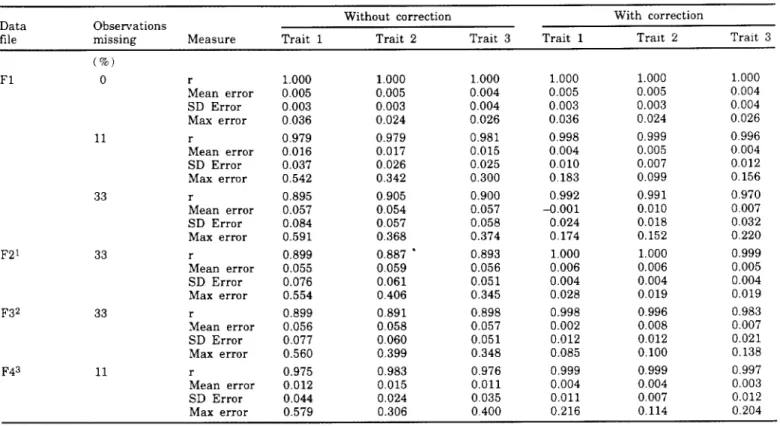
Table 1 shows correlations, mean errors, standard deviations of errors, and maximum absolute errors between approximate and exact reliabilities for simu-lated data observed for all the animals, with and without the correction for missing traits. With no missing observations (data file F1), approximate
TABLE 1. Correlations (r) between exact reliabilities from multiple-trait direct inversion and reliabilities from multiple-trait approxima-tion by multiple diagonalizaapproxima-tion for simulated data with and without correcapproxima-tion for missing observaapproxima-tions, mean errors of approximaapproxima-tion (mean error), standard deviation of errors (SD error), and maximum absolute errors (max error) observed for all animals.
Without correction With correction
Data Observations
file missing Measure Trait 1 Trait 2 Trait 3 Trait 1 TraIt 2 Trait 3
(%) F1 0 r 1.000 1.000 1.000 1.000 1.000 1.000 Mean error 0.005 0.005 0.004 0.005 0.005 0.004 SD Error 0.003 0.003 0.004 0.003 0.003 0.004 Max error 0036 0.024 0.026 0.036 0.024 0.026 11 r 0.979 0.979 0.981 0.998 0.999 0.996 Mean error 0016 0.017 0.015 0.004 0.005 0.004 SD Error 0.037 0.026 0.025 0.010 0.007 0012 Max error 0.542 0.342 0.300 0.183 0.099 0.156 33 r 0.895 0.905 0.900 0.992 0.991 0970
Mean error 0.057 0.054 0.057 -D.OOI 0.010 0.007
SD Error 0.084 0.057 0.058 0.024 0.018 0.032 Max error 0.591 0.368 0.374 0.174 0.152 0.220 F21 33 r 0.899 0.887 • 0.893 1.000 1.000 0.999 Mean error 0.055 0.059 0.056 0.006 0.006 0.005 SD Error 0.076 0.061 0.051 0.004 0.004 0.004 Max error 0.554 0.406 0.345 0.028 0.019 0.019 F3 2 33 r 0.899 0.891 0.898 0.998 0.996 0.983 Mean error 0.056 0.058 0.057 0.002 0.008 0.007 SD Error 0.077 0.060 0.051 0.012 0.012 0.021 Max error 0.560 0.399 0.348 0.085 0.100 0.138 F43 11 r 0.975 0.983 0.976 0.999 0.999 0.997 Mean error 0.012 0.015 0.011 0.004 0.004 0.003 SD Error 0.044 0.024 0035 0.011 0.007 0.012
Max error 0.579 0.306 OAOO 0.216 0.114 0.204
lCovariances are 0.1 times those for data file F1. 2Covariances are 0.5 times those for data file F1. 3Covariances are 1.4 times those for data file F1.
Journal of Dairy Science Vol. 79, No.2, 1996
sity, Ithaca, New York, 1994, personal communica-tion): [ 7.9 21.1 11.8] Go
=
21.1 236.8 103.7 , 11.8 103.7 174.6 and [ 12.4 15.3 10.1] Ho=
15.3 588.6 -91.9 . 10.1 -91.9 496.7Missing data (43% of observations) were essentially all grouped in specific classes for fixed effects, unlike the dairy data, for which only 9% of missing observa-tions were concentrated in recent herd-year-seasons.
Method of comparison. Approximate reliabilities
were calculated with the algorithm that corrects for missing values and with the normal algorithm that ignores missing data; then those approximate values
were compared with exact reliabilities obtained from a direct inversion approach by MTDFREML (1), a package using the SPARSPAK sparse matrix solver (2), which was modified to obtain the reliabilities. For field data files, single-trait reliabilities were cal-culated using the same algorithm but ignoring (co)variances between traits. Accuracy of the methods was assessed by Pearson's correlation be-tween approximated and exact reliabilities and by means, standard deviations, and maxima of the ap-proximation error, computed separately for all animals, animals with records, and sires of animals with records.
RESULTS AND DISCUSSION
Table 1 shows correlations, mean errors, standard deviations of errors, and maximum absolute errors between approximate and exact reliabilities for simu-lated data observed for all the animals, with and without the correction for missing traits. With no missing observations (data file F1), approximate
TABLE 1. Correlations (r) between exact reliabilities from multiple-trait direct inversion and reliabilities from multiple-trait approxima-tion by multiple diagonalizaapproxima-tion for simulated data with and without correcapproxima-tion for missing observaapproxima-tions, mean errors of approximaapproxima-tion (mean error), standard deviation of errors (SD error), and maximum absolute errors (max error) observed for all animals.
Without correction With correction
Data Observations
file missing Measure Trait 1 Trait 2 Trait 3 Trait 1 TraIt 2 Trait 3
(%) F1 0 r 1.000 1.000 1.000 1.000 1.000 1.000 Mean error 0.005 0.005 0.004 0.005 0.005 0.004 SD Error 0.003 0.003 0.004 0.003 0.003 0.004 Max error 0036 0.024 0.026 0.036 0.024 0.026 11 r 0.979 0.979 0.981 0.998 0.999 0.996 Mean error 0016 0.017 0.015 0.004 0.005 0.004 SD Error 0.037 0.026 0.025 0.010 0.007 0012 Max error 0.542 0.342 0.300 0.183 0.099 0.156 33 r 0.895 0.905 0.900 0.992 0.991 0970
Mean error 0.057 0.054 0.057 -D.OOI 0.010 0.007
SD Error 0.084 0.057 0.058 0.024 0.018 0.032 Max error 0.591 0.368 0.374 0.174 0.152 0.220 F21 33 r 0.899 0.887 • 0.893 1.000 1.000 0.999 Mean error 0.055 0.059 0.056 0.006 0.006 0.005 SD Error 0.076 0.061 0.051 0.004 0.004 0.004 Max error 0.554 0.406 0.345 0.028 0.019 0.019 F3 2 33 r 0.899 0.891 0.898 0.998 0.996 0.983 Mean error 0.056 0.058 0.057 0.002 0.008 0.007 SD Error 0.077 0.060 0.051 0.012 0.012 0.021 Max error 0.560 0.399 0.348 0.085 0.100 0.138 F43 11 r 0.975 0.983 0.976 0.999 0.999 0.997 Mean error 0.012 0.015 0.011 0.004 0.004 0.003 SD Error 0.044 0.024 0035 0.011 0.007 0.012
Max error 0.579 0.306 OAOO 0.216 0.114 0.204
lCovariances are 0.1 times those for data file F1. 2Covariances are 0.5 times those for data file F1. 3Covariances are 1.4 times those for data file F1.
reliabilities were close to exact reliabiIities from direct inversion.
The improvement with the correction was most dramatic for simulated data with extremely low covariances among traits (data file F2). The improve-ment with the correction was smaller for data with higher covariances between traits. Thus, the al-gorithm works best with fewer missing observations and low correlations between traits. This last fact is obvious because Equation [15] is only an approxima-tion because of discarded off-diagonals.
Tables 2 and 3 show values for the same measures observed for animals with records and for sires of animals with records. The minimum correlation for animals with records without the correction is only 0.408, but for sires it is never <0.969. After the correc-tions, these correlations increase to 0.888 and 0.992, which suggests that, although the correction for miss-ing data helped the reliability approximation for animals with records, these approximations were still not as good as for sires with several progeny.
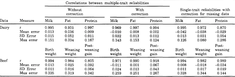
Also, for the field data for dairy cattle, correlations between approximate and exact reliabilities (Table 4) were much higher than for simulated data. For milk and protein yields, they were >0.990, even without the use of the algorithm for the correction for missing data. The correction has increased the corre-lations for fat from 0.931 to 0.997, marginally decreased the correlation for protein, and reduced the correlation for milk from 0.995 to 0.969. The correc-tion changed bias for milk from 0.013 to -0.010, mean-ing that reliability for milk changed from generally being overestimated to being underestimated, The single-trait approximation had a bias up to four times higher than the multiple-trait approximation with the correction, but the standard deviation of the single-trait approximation was better for milk, the only single-trait that was always recorded; the maximum error was smaller for milk and fat. Relatively modest gains from the correction in yield traits were likely caused by high correlations among the traits.
The most accurate method for beef data was the single-trait approach. The correction in the multitrait
TABLE 2, Correlations (r) between exact reliabilities from multiple-trait direct inversion and reliabilities from multiple-trait approxima-tion by multiple diagonalizaapproxima-tion for simulated data with and without correcapproxima-tion for missing observaapproxima-tions, mean errors of approximaapproxima-tion (mean errorl, standard deviation of errors (SD error), and maximum absolute errors (max error) observed for all animals with records,
Observations Without correction With correction
Data
me missing Measure Trait 1 Trait 2 Trait 3 Trait 1 Trait 2 Trait 3
(%) F1 0 r 0.995 0.995 0.995 0.995 0,995 0.995 Mean error 0,005 0,005 0,005 0.005 0.005 0.005 SO Error 0.003 0.003 0,003 0.003 0.003 0.003 Max error 0.012 0.012 0011 0.012 0.012 0,011 11 r 0,656 0.831 0,778 0,978 0,993 0,955 Mean error 0.019 0.020 0.018 0.004 0,006 0,004 SO Error 0.043 0.031 0.029 0.012 0.007 0,014 Max error 0.542 0.342 0.300 0.183 0,099 0,156 33 r 0,549 0,651 0,619 0.968 0.980 0.888 Mean error 0.068 0,063 0,067 -0.001 0.011 0.008 SD Error 0,098 0,065 0,067 0.028 0.021 0,038 Max error 0.590 0.368 0,374 0,174 0.152 0,220 F21 33 r 0.576 0.625 0.638 1,000 0,999 0,999 Mean error 0.065 0,068 0.065 0.007 0.006 0,006 SO Error 0,088 0,070 0,057 0.003 0.003 0.004 Max error 0,554 0.406 0,345 0.019 0.019 0.019 F32 33 r 0,571 0,631 0,642 0,993 0.993 0,950 Mean error 0,066 0.067 0,066 0.002 0,010 0.008 SO Error 0.090 0,069 0.058 0,014 0.013 0,025 Max error 0.560 0.399 0.348 0.085 0,100 0.138 F43 11 r 0.408 0,844 0.519 0.975 0.989 0.957 Mean error 0,014 0,017 0,014 0.004 0.005 0.004 SD Error 0.052 0,028 0,042 0.012 0.008 0.014 Max error 0,579 0.306 0.400 0.216 0.114 0,204
lCovariances are 0,1 times those for data tile Fl. 2Covariances are 0.5 times those for data tile Fl. 3Covariances are 1.4 times those for data tile Fl.
reliabilities were close to exact reliabiIities from direct inversion.
The improvement with the correction was most dramatic for simulated data with extremely low covariances among traits (data file F2). The improve-ment with the correction was smaller for data with higher covariances between traits. Thus, the al-gorithm works best with fewer missing observations and low correlations between traits. This last fact is obvious because Equation [15] is only an approxima-tion because of discarded off-diagonals.
Tables 2 and 3 show values for the same measures observed for animals with records and for sires of animals with records. The minimum correlation for animals with records without the correction is only 0.408, but for sires it is never <0.969. After the correc-tions, these correlations increase to 0.888 and 0.992, which suggests that, although the correction for miss-ing data helped the reliability approximation for animals with records, these approximations were still not as good as for sires with several progeny.
Also, for the field data for dairy cattle, correlations between approximate and exact reliabilities (Table 4) were much higher than for simulated data. For milk and protein yields, they were >0.990, even without the use of the algorithm for the correction for missing data. The correction has increased the corre-lations for fat from 0.931 to 0.997, marginally decreased the correlation for protein, and reduced the correlation for milk from 0.995 to 0.969. The correc-tion changed bias for milk from 0.013 to -0.010, mean-ing that reliability for milk changed from generally being overestimated to being underestimated, The single-trait approximation had a bias up to four times higher than the multiple-trait approximation with the correction, but the standard deviation of the single-trait approximation was better for milk, the only single-trait that was always recorded; the maximum error was smaller for milk and fat. Relatively modest gains from the correction in yield traits were likely caused by high correlations among the traits.
The most accurate method for beef data was the single-trait approach. The correction in the multitrait
TABLE 2, Correlations (r) between exact reliabilities from multiple-trait direct inversion and reliabilities from multiple-trait approxima-tion by multiple diagonalizaapproxima-tion for simulated data with and without correcapproxima-tion for missing observaapproxima-tions, mean errors of approximaapproxima-tion (mean errorl, standard deviation of errors (SD error), and maximum absolute errors (max error) observed for all animals with records,
Observations Without correction With correction
Data
me missing Measure Trait 1 Trait 2 Trait 3 Trait 1 Trait 2 Trait 3
(%) F1 0 r 0.995 0.995 0.995 0.995 0,995 0.995 Mean error 0,005 0,005 0,005 0.005 0.005 0.005 SO Error 0.003 0.003 0,003 0.003 0.003 0.003 Max error 0.012 0.012 0011 0.012 0.012 0,011 11 r 0,656 0.831 0,778 0,978 0,993 0,955 Mean error 0.019 0.020 0.018 0.004 0,006 0,004 SO Error 0.043 0.031 0.029 0.012 0.007 0,014 Max error 0.542 0.342 0.300 0.183 0,099 0,156 33 r 0,549 0,651 0,619 0.968 0.980 0.888 Mean error 0.068 0,063 0,067 -0.001 0.011 0.008 SD Error 0,098 0,065 0,067 0.028 0.021 0,038 Max error 0.590 0.368 0,374 0,174 0.152 0,220 F21 33 r 0.576 0.625 0.638 1,000 0,999 0,999 Mean error 0.065 0,068 0.065 0.007 0.006 0,006 SO Error 0,088 0,070 0,057 0.003 0.003 0.004 Max error 0,554 0.406 0,345 0.019 0.019 0.019 F32 33 r 0,571 0,631 0,642 0,993 0.993 0,950 Mean error 0,066 0.067 0,066 0.002 0,010 0.008 SO Error 0.090 0,069 0.058 0,014 0.013 0,025 Max error 0.560 0.399 0.348 0.085 0,100 0.138 F43 11 r 0.408 0,844 0.519 0.975 0.989 0.957 Mean error 0,014 0,017 0,014 0.004 0.005 0.004 SD Error 0.052 0,028 0,042 0.012 0.008 0.014 Max error 0,579 0.306 0.400 0.216 0.114 0,204
lCovariances are 0,1 times those for data tile Fl. 2Covariances are 0.5 times those for data tile Fl. 3Covariances are 1.4 times those for data tile Fl.
324
TABLE 3. Correlations (r) between exact reliabilities from multiple-trait direct inversion and reliabilities from multiple-trait approxima-tion by multiple diagonalizaapproxima-tion for simulated data with and without correcapproxima-tion for missing observaapproxima-tions, mean errors of approximaapproxima-tion (mean error), standard deviation of errors (SD error), and maximum absolute errors (max error) observed for sires of animals with records.
Data Observations Without correction With correction
file missing Measure Trait 1 Trait 2 Trait 3 Trait 1 Trait 2 Trait 3
(%) Fl 0 r 0.999 0.999 0.999 0.999 0.999 0999 Mean error 0.005 0005 0.004 0.005 0.005 0.004 SD Error 0.003 0,003 0.003 0.003 0.003 0.003 Max error 0.024 0.024 0.019 0.024 0.024 0.019 11 r 0,993 0.994 0.996 0.999 0.999 0.998 Mean error 0.011 0.014 0.012 0,004 0.005 0004 SD Error 0.011 0.011 0.008 0,005 0.004 0006 Max error 0.141 0.091 0.059 0.047 0.025 0.029 33 r 0.969 0.980 0.978 0.996 0.998 0.992 Mean error 0.038 0.042 0.041 0.000 0.009 0.005 SD Error 0.025 0.019 0.018 0.009 0.007 0.011 Max error 0.177 0.091 0.097 0.032 0.028 0.039 F21 33 r 0.970 0.974 0.975 1.000 0,999 0.999 Mean error 0.039 0.046 0.046 0.005 0.005 0.005 SD Error 0.025 0.022 0.021 0.003 0.004 0.003 Max error 0.182 0.103 0.118 0.020 0.019 0.015 F32 33 r 0.971 0.976 0.976 0.999 0.999 0.996 Mean error 0.039 0.045 0026 0.002 0.007 0.005 SD Error 0.025 0.021 0.020 0.005 0.005 0.008 Max error 0.180 0.104 0.111 0.023 0.026 0.033 F43 11 r 0.992 0.995 0995 0.998 0.999 0.998 Mean error 0.009 0.013 0.009 0.004 0.004 0.003 SD Error 0.012 0.010 0.008 0.006 0.004 0.005 Max error 0.147 0.078 0.054 0.055 0.019 0,022
lCovariances are 0.1 times those for data file F1. 2Covariances are 0.5 times those for data file F1. 3Covariances are 1.4 times those for data file Fl.
TABLE 4. Correlations (r) between exact reliabilities from multiple-trait direct inversion and reliabilities from multiple-trait approxima-tion by multiple diagonalizaapproxima-tion for field data with and without correcapproxima-tion for missing observaapproxima-tions and single-trait reliabilities obtained by ignoring covariances between traits; mean errors of approximation (mean error), standard deviation of errors (SD error) and maximum absolute errors (max error), measures observed for all the animals.
Correlations between multiple-trait reliabilities
Without With Single-trait reliabilities with
correction correction correction for missing data
Data Measure Milk Fat Protein Milk Fat Protein Milk Fat Protein
Dairy r 0.995 0.931 0.997 0969 0.997 0.994 0.995 0.972 0.870
Mean error 0.013 0.036 0.009 -0.010 0.008 0.002 -0.042 -0.038 -0.029
SD Error 0.015 0.052 0.011 0.032 0.013 0.012 0.013 0.031 0.054
Max error 0.151 0.334 0.167 0.143 0.153 0.124 0.126 0.080 0.286
Post- Post-
Post-Birth Weaning weaning Birth Weaning weaning Birth Weaning weaning
weight weight gain weight weight gain weight weight gain
Beef r 0.994 0984 0.805 0.971 0.990 0.918 0.994 0.982 0.989
Mean error 0,013 0025 0.092 -0.011 0.001 0.067 0.008 -0.018 -0.034
SD Error 0.011 0.016 0.064 0.024 0.013 0.043 0.011 0.017 0.019
Max error 0.335 0.319 0.342 0.259 0.251 0.267 0.328 0.344 0.144
Journal of Dairy Science Vol. 79, No, 2, 1996 324
TABLE 3. Correlations (r) between exact reliabilities from multiple-trait direct inversion and reliabilities from multiple-trait approxima-tion by multiple diagonalizaapproxima-tion for simulated data with and without correcapproxima-tion for missing observaapproxima-tions, mean errors of approximaapproxima-tion (mean error), standard deviation of errors (SD error), and maximum absolute errors (max error) observed for sires of animals with records.
Data Observations Without correction With correction
file missing Measure Trait 1 Trait 2 Trait 3 Trait 1 Trait 2 Trait 3
(%) Fl 0 r 0.999 0.999 0.999 0.999 0.999 0999 Mean error 0.005 0005 0.004 0.005 0.005 0.004 SD Error 0.003 0,003 0.003 0.003 0.003 0.003 Max error 0.024 0.024 0.019 0.024 0.024 0.019 11 r 0,993 0.994 0.996 0.999 0.999 0.998 Mean error 0.011 0.014 0.012 0,004 0.005 0004 SD Error 0.011 0.011 0.008 0,005 0.004 0006 Max error 0.141 0.091 0.059 0.047 0.025 0.029 33 r 0.969 0.980 0.978 0.996 0.998 0.992 Mean error 0.038 0.042 0.041 0.000 0.009 0.005 SD Error 0.025 0.019 0.018 0.009 0.007 0.011 Max error 0.177 0.091 0.097 0.032 0.028 0.039 F21 33 r 0.970 0.974 0.975 1.000 0,999 0.999 Mean error 0.039 0.046 0.046 0.005 0.005 0.005 SD Error 0.025 0.022 0.021 0.003 0.004 0.003 Max error 0.182 0.103 0.118 0.020 0.019 0.015 F32 33 r 0.971 0.976 0.976 0.999 0.999 0.996 Mean error 0.039 0.045 0026 0.002 0.007 0.005 SD Error 0.025 0.021 0.020 0.005 0.005 0.008 Max error 0.180 0.104 0.111 0.023 0.026 0.033 F43 11 r 0.992 0.995 0995 0.998 0.999 0.998 Mean error 0.009 0.013 0.009 0.004 0.004 0.003 SD Error 0.012 0.010 0.008 0.006 0.004 0.005 Max error 0.147 0.078 0.054 0.055 0.019 0,022
lCovariances are 0.1 times those for data file F1. 2Covariances are 0.5 times those for data file F1. 3Covariances are 1.4 times those for data file Fl.
TABLE 4. Correlations (r) between exact reliabilities from multiple-trait direct inversion and reliabilities from multiple-trait approxima-tion by multiple diagonalizaapproxima-tion for field data with and without correcapproxima-tion for missing observaapproxima-tions and single-trait reliabilities obtained by ignoring covariances between traits; mean errors of approximation (mean error), standard deviation of errors (SD error) and maximum absolute errors (max error), measures observed for all the animals.
Correlations between multiple-trait reliabilities
Without With Single-trait reliabilities with
correction correction correction for missing data
Data Measure Milk Fat Protein Milk Fat Protein Milk Fat Protein
Dairy r 0.995 0.931 0.997 0969 0.997 0.994 0.995 0.972 0.870
Mean error 0.013 0.036 0.009 -0.010 0.008 0.002 -0.042 -0.038 -0.029
SD Error 0.015 0.052 0.011 0.032 0.013 0.012 0.013 0.031 0.054
Max error 0.151 0.334 0.167 0.143 0.153 0.124 0.126 0.080 0.286
Post- Post-
Post-Birth Weaning weaning Birth Weaning weaning Birth Weaning weaning
weight weight gain weight weight gain weight weight gain
Beef r 0.994 0984 0.805 0.971 0.990 0.918 0.994 0.982 0.989
Mean error 0,013 0025 0.092 -0.011 0.001 0.067 0.008 -0.018 -0.034
SD Error 0.011 0.016 0.064 0.024 0.013 0.043 0.011 0.017 0.019
Max error 0.335 0.319 0.342 0.259 0.251 0.267 0.328 0.344 0.144
TABLE 5. Correlations (r) between exact reliabilities from multiple-trait direct inversion and reliabilities from multiple-trait approxima-tion by multiple diagonalizaapproxima-tion for field data with and without correcapproxima-tion for missing observaapproxima-tions and smgle-trait reliabilities obtained by ignoring covariances between traits; mean errors of approximation (mean error), standard deviation of errors (SD error, and maximum absolute errors (max error), measures observed for animals with records
Data Dairy
Beef
Correlations between multiple-trait reliabilities
Without With Single-trait reliabilities with
correction correction correction for missing data
Measure :\1ilk Fat Protein Milk Fat Protein Milk Fat Protein
r 0.981 0.785 0.990 0.900 0.992 0.982 0.980 0.970 0.738
Mean error 0.019 0.054 0013 -0.014 0013 0.002 -0007 -0.041 -0.042
SD Error 0.014 0.059 0.01l 0.040 0012 0.014 0.015 0.033 0.066
Max error 0.151 0.334 0167 0.143 0.153 0.124 0.126 0.160 0.286
Post- Post- Post·
Birth Weaning weaning Birth Weaning weaning Birth Weaning weaning
weight weight gain weight weight gain weight weight gain
r 0.986 0.964 0711 0.933 0980 0.902 0.986 0.963 0.992
Mean error 0.014 0.025 0.094 -0.012 0.001 0.068 0.008 -0.019 -0.035
SD Error 0009 0.016 0.065 0.024 0.013 0.044 0.009 0.016 0017
Max error 0.147 0.172 0.3ll 0.101 0.104 0.248 0.138 0.108 0121
model has decreased bias and maximum error for all traits, but the standard errors actually increased from 0.011 to 0.024, and the correlation for postweaning gain was only 0.918. The failure of the correction could be due to an inability to account for missing management classes.
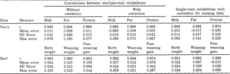
Tables 5 and 6 show the results for animals with records and sires of animals with records. As for simulated data, the correction is much better for sires than for cows. Correlations for sires were all >0.99, which was better than with the single-trait model for which the correlation for protein was 0.974. Correla-tions for sires with beef data were all >0.97; however,
the correlations by the single-trait model were all >0.99. One explanation for the different behavior ob·· served for the three types of data files is the different distribution of missing values for the fixed effects. For the simulated data files, missing values were not grouped in complete empty levels of the fixed effect. For the field data for dairy cattle, 9% of the missing values were concentrated in certain herd-year-season classes, and, for the field data for beef cattle, neacly all missing data were concentrated in certain fixed effect classes. This result suggests that the algorithm is less accurate if complete classes of fixed effects were missing.
TABLE 6. Correlations (r) between exact reliabilities from multiple-trait direct inversion and reliabilities from multiple-trait approxima-tion by multiple diagonalizaapproxima-tion for field data with and without correcapproxima-tion for missing observaapproxima-tions and single-trait reliabilities obtained by ignoring covariances between traits; mean errors of approximation (mean error), standard deviation of errors (SD error, and maximum absolute errors (max error), measures observed for sires of animals with records.
Data Dairy
Beef
Correlations between multiple-trait reliabilities
Without With Single-trait reliabilities with
correction correction correction for missing data
Measure Milk Fat Protein Milk Fat Protein Milk Fat Protein
r 0.998 0.986 0.998 0.993 0.998 0.998 0.998 0.992 0.974
Mean error 0.011 0.029 0.011 -0.005 0.009 0.005 0.002 -0.017 -0.020
SD Error 0.013 0.026 0.013 0.018 0.013 0.012 0.01l 0.017 0.028
Max error 0.079 0.190 0.077 0.085 0.073 0.067 0.062 0.141 0.223
Post- Post-
Post-Birth Weaning weaning Birth Weaning weaning Birth Weaning weaning
weight weight gain weight weight gain weight weight gain
r 0.991 0.992 0.954 0.992 0.994 0.974 0.991 0.992 0.996
Mean error 0.024 0.030 0.100 0.007 0.012 0.079 0.022 0.007 -0.010
SD Error 0.024 0.023 0.056 0.024 0021 0.042 0.024 0.026 0.028
Max error 0.335 0.319 0.342 0.259 0251 0.267 0.328 0.264 0.095
TABLE 5. Correlations (r) between exact reliabilities from multiple-trait direct inversion and reliabilities from multiple-trait approxima-tion by multiple diagonalizaapproxima-tion for field data with and without correcapproxima-tion for missing observaapproxima-tions and smgle-trait reliabilities obtained by ignoring covariances between traits; mean errors of approximation (mean error), standard deviation of errors (SD error, and maximum absolute errors (max error), measures observed for animals with records
Data Dairy
Beef
Correlations between multiple-trait reliabilities
Without With Single-trait reliabilities with
correction correction correction for missing data
Measure :\1ilk Fat Protein Milk Fat Protein Milk Fat Protein
r 0.981 0.785 0.990 0.900 0.992 0.982 0.980 0.970 0.738
Mean error 0.019 0.054 0013 -0.014 0013 0.002 -0007 -0.041 -0.042
SD Error 0.014 0.059 0.01l 0.040 0012 0.014 0.015 0.033 0.066
Max error 0.151 0.334 0167 0.143 0.153 0.124 0.126 0.160 0.286
Post- Post- Post·
Birth Weaning weaning Birth Weaning weaning Birth Weaning weaning
weight weight gain weight weight gain weight weight gain
r 0.986 0.964 0711 0.933 0980 0.902 0.986 0.963 0.992
Mean error 0.014 0.025 0.094 -0.012 0.001 0.068 0.008 -0.019 -0.035
SD Error 0009 0.016 0.065 0.024 0.013 0.044 0.009 0.016 0017
Max error 0.147 0.172 0.3ll 0.101 0.104 0.248 0.138 0.108 0121
model has decreased bias and maximum error for all traits, but the standard errors actually increased from 0.011 to 0.024, and the correlation for postweaning gain was only 0.918. The failure of the correction could be due to an inability to account for missing management classes.
Tables 5 and 6 show the results for animals with records and sires of animals with records. As for simulated data, the correction is much better for sires than for cows. Correlations for sires were all >0.99, which was better than with the single-trait model for which the correlation for protein was 0.974. Correla-tions for sires with beef data were all >0.97; however,
the correlations by the single-trait model were all >0.99. One explanation for the different behavior ob·· served for the three types of data files is the different distribution of missing values for the fixed effects. For the simulated data files, missing values were not grouped in complete empty levels of the fixed effect. For the field data for dairy cattle, 9% of the missing values were concentrated in certain herd-year-season classes, and, for the field data for beef cattle, neacly all missing data were concentrated in certain fixed effect classes. This result suggests that the algorithm is less accurate if complete classes of fixed effects were missing.
TABLE 6. Correlations (r) between exact reliabilities from multiple-trait direct inversion and reliabilities from multiple-trait approxima-tion by multiple diagonalizaapproxima-tion for field data with and without correcapproxima-tion for missing observaapproxima-tions and single-trait reliabilities obtained by ignoring covariances between traits; mean errors of approximation (mean error), standard deviation of errors (SD error, and maximum absolute errors (max error), measures observed for sires of animals with records.
Data Dairy
Beef
Correlations between multiple-trait reliabilities
Without With Single-trait reliabilities with
correction correction correction for missing data
Measure Milk Fat Protein Milk Fat Protein Milk Fat Protein
r 0.998 0.986 0.998 0.993 0.998 0.998 0.998 0.992 0.974
Mean error 0.011 0.029 0.011 -0.005 0.009 0.005 0.002 -0.017 -0.020
SD Error 0.013 0.026 0.013 0.018 0.013 0.012 0.01l 0.017 0.028
Max error 0.079 0.190 0.077 0.085 0.073 0.067 0.062 0.141 0.223
Post- Post-
Post-Birth Weaning weaning Birth Weaning weaning Birth Weaning weaning
weight weight gain weight weight gain weight weight gain
r 0.991 0.992 0.954 0.992 0.994 0.974 0.991 0.992 0.996
Mean error 0.024 0.030 0.100 0.007 0.012 0.079 0.022 0.007 -0.010
SD Error 0.024 0.023 0.056 0.024 0021 0.042 0.024 0.026 0.028
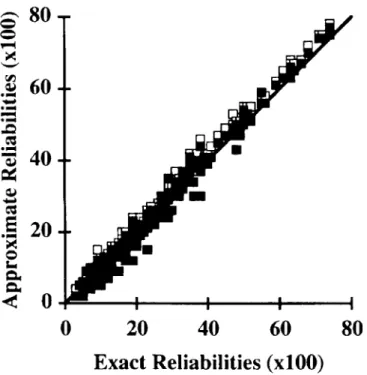
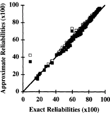
Figure 1. Plot of exact versus approximate reliabilities for milk yield obtained by multiple diagonalization with (.) and without (0) correction for missing data for sires of cows with records.
Exact Reliabilities (xlOO)
-- 80
=
=
~ ~--
rI'J .~60
-
.
-.-
.c
eo:
.-
Qj40
==:
QJ-
eo:
.5
20
~o
'"'
c..
c..
<
0
o
20
40
60
80
Figures 1, 2, and 3 show plots of approximate versus exact reliabilities for sires of cows with records for milk yield traits. For most sires, the multitrait approximation overestimated the reliabilities, and the correction has reduced that overestimation. The un-derestimation occurred only for lower repeatability sires «55%), suggesting that the approximation does not affect sires with more offspring. Except for milk yield, for which certain values were slightly overcor-rected, those corrected values were close to the exact reliabilities. Figures 4, 5, and 6 show plots of approxi-mates versus exact reliabilities for sires of animals with beef records. For birth weight and weaning weight, the multitrait approximation overestimated slightly the reliabilities for most animals, and the correction for missing values reduced that overesti-mation. The approximations were worse for two sires that had progeny in fewer herds than other sires and whose relationships were less complete. For certain animals, values were slightly overcorrected. For post-weaning gain, multitrait approximation showed big estimation errors. The correction reduced these er-rors, but not as much as for the two other traits. A systematic bias existed for animals with high exact reliabilities, and approximate reliabilities were over-estimated.
--
80
-- 80
=
~
=
~ ~ il< ~--
rI'J--60
rI'J60
QJ....
QJ....
-
.-
-....
--
....
....
.c
,.Qeo:
....
eo:
....
40
-
40
-
QJ QJ==:
==:
QJ-
QJ-
eo:
eo:
e
e
20
....
20
....
~ ~ 0 0'"'
'"'
c..
Q.c..
c..
<
0
<
0
0
20
40
60
80
0
20
40
60
80
Exact Reliabilities (xlOO)
Exact Reliabilities (xlOO)
Figure 2. Plot of exact versus approximate reliabilities for fat yield obtained by multiple diagonalization with (.) and without (0) correction for missing data for sires of cows with records.
Journal of Dairy Science Vol. 79, No.2, 1996
Figure 3. Plot of exact versus approximate reliabilities for pro-tein yield obtained by multiple diagonalization with (.) and without (0) correction for missing data for sires of cows with records.