A Structural Model for Early Exit of Older Men in
Belgium
Mathieu Lefebvre
HEC-ULg, University of Liège, Belgium
E-mail: mathieu.lefebvre@ulg.ac.be
Kristian Orsini
European Commission, Brussels, Belgium
e-mail: kristian.orsini@ec.europa.eu Abstract
In this paper we propose a structural model of the retirement decision for older workers in Belgium. We model the exit paths available through the various available schemes. Our framework allows exploiting all information
on possible exit paths and also better identifying preferences and constraints. Results based upon Belgian microsimulation data from 2001 for private sector workers fits rather well observed behavior. Simulations of
hypothetical reforms illustrate the potential effects of changing social security rules.
Keywords: Retirement, social security reforms, microsimulation. JEL Classification: C15, C51, D91, J26, E17.
1. Introduction
In this paper, we develop a structural model of the retirement decision in Belgium. The last decades have shown a substantial decline in labor force participation of older workers in OECD countries but Belgium has been experiencing this trend most severely than others. The labor force participation of men aged 60-64 fell from 61% in 1970 to 20% in 2003 while that of men aged 55-59 fell from 82% to 54%.
Previous studies by Pestieau and Stijns (1999) and Dellis et al. (2004) have stressed the role of the social security system in inducing early retirement in Belgium. Since the early 1970's, a large variety of exit schemes have been put in place. The standard retirement path requiring workers to be at least 60 years old has been paralleled by an early retirement scheme for workers aged 58 and over1 and by a derogation to standard requirements for old-age unemployment, assuring a smooth transition from unemployment to retirement (the so called "Canada-dry" system2).
The aim of this paper is to propose a structural model of the labor supply of older workers in Belgium. The analysis is based on a dynamic discrete choice model, which includes individual heterogeneity in the deterministic part of the utility. In essence our model is similar to the option value model by Stock and Wise (1990). In the option value model, a worker chooses the state that has the highest value by comparing the expected discounted value of the income they will receive until the end of life under different strategies.
However in several respects, our modeling strategy extends the option value approach. The intertemporal budget constraint is fully modeled, thus exploiting all the available information. Observed individual or family characteristics are
incorporated through one or more of the coefficients of the utility function. We also exploit all information on possible exit paths and our framework allows better identifying preferences and constraints. The model recovers the parameters of the structural preferences of the population. Finally one advantage of this modeling is
1 This is the statutory age specified in the law but many departures from this, authorizing an exit
even earlier are possible within the framework of sector-level collective agreements.
2 This alludes to an old European commercial for Canada Dry ginger ale which was said to have
that it is much more practical than the dynamic programming rule developed to implement the dynamic choice of labor supply3.
We estimate the model for Belgium by using a unique dataset for the year 2001 derived from the microsimulation model MIMOSIS; a static simulation model based on administrative information. The microsimulation model allows the reconstruction of the individual intertemporal budget constraint of wage-earners. Difficulties are encountered in modeling the building up of social security wealth for civil servants and the self employed. We therefore focus on the behavior of wage-earners. As stressed in Coile and Gruber (2007), retirement decisions are a function of both pension incentives and wages, with wages being the source of most of the variation between individuals. If wage differences between
individuals partly capture heterogeneity in tastes for work, however, then building wage variation into the retirement incentive measure can lead to misleading estimates of the responsiveness to financial incentives. The use of our much richer data source will avoid this problem, by controlling comprehensively for past earnings and individual household characteristics.
In the following section we detail the various pathways to retirement for wage-earners in Belgium. The model is presented in Section 3. Data, sample selection and prior-estimation computations are described in Section 4. Parameter estimates are presented in Section 5. Finally, in Section 6, simulations of illustrative
changes in the social security system are presented. Section 7 concludes.
2. Institutional features
The Belgian retirement system is characterized by three very unequal pillars4. First comes the wage-earners' retirement scheme which represents the largest proportion of pension income for the vast majority of individuals. The second pillar consists of company pension plans, which only play a minor role as a source of income for the average worker. In the private sector they are confined to the higher-income individuals. The third pillar is made up of individual retirement savings, which take the form of individual-pension savings account, life insurance
3 See Berkovec and Stern (1991), Rust (1989) and Rust and Phelan (1997) for dynamic
programming models of retirement behavior. A major inconvenient of the dynamic programming models is that they are computationally intensive.
4 A good review of the various Belgian social security schemes can be found in Dellis et al.
and so forth. In this paper we focus exclusively on the first pillar. Private programs are very small in size and they account for a much lower share of the retiree’s income. Whereas the first pillar represents pension entitlements of more than 250 % of GDP, assets in private-pension funds only amount to 10% of GDP. Alongside the wage-earners' retirement scheme, several other pathways into retirement have progressively evolved. They operate under the name of conventional early retirement schemes or alternatively as a form of old-age unemployment. We will review these three schemes.
2.1. The Wage-Earners’ Retirement Scheme
This is the standard retirement scheme. It allows voluntary retirement from age 60, with a normal retirement age fixed at 65. The choice of retirement age does not imply any actuarial adjustment. However the choice of retirement age is not completely neutral with respect to the benefit amount, because a full earnings history consists of forty-five years of work for men, a condition that many people do not satisfy at the age of 60. For those having more than forty-five working years, a dropout-year provision operates, replacing low-income years with higher ones. Benefits (B) are computed according to the formula:
k w N
n
B= * *
where n represents the number of years of affiliation with the scheme, N the number of years required for a full career, and k is a replacement rate, which takes the value of 0.6 or 0.75 depending on whether the individual claims benefits as a single person or as a household. w is the indexed average wage over the period of affiliation. A peculiar feature of the system is that periods of one’s life spent on replacement income (such as unemployment or disability benefits) fully count as years worked in the computation of the average wage, and hence of the social security benefits. For any such periods, fictive wages are inserted into the average wage computation. Imputed wages are set equal in real terms to those the worker earned before entering these replacement income programs. Finally benefits are shielded against inflation through an automatic consumer price index adjustment and are subject to an earnings test. Currently the earnings limit is approximately €7,422 per year. For earnings above this limit, pension entitlement is suspended.
A guaranteed minimum pension income is fully paid out of general government revenue and it is means-tested. This pension is only available after the normal retirement age of 65.
2.2. The Conventional early Retirement Scheme
There is a whole arsenal of early retirement schemes that have been put in place over the last few decades. These schemes are gathered together under the title of
Conventional Early Retirement (Prépension conventionelle). All of these
arrangements are based on collective agreements, which are negotiated between employee and employer associations. Within such schemes, the workers exit the labor market and receive unemployment compensation and a bonus paid by the employer, which equals half the difference between the individual's last net wage and the unemployment benefit. The amount of unemployment benefit depends on the family status. If the individual is single or has a family which is dependent on her earnings, she is entitled to 60 per cent of the previous net wage. If the spouse or partner has income, she may claim only 55 per cent.
Early retirement scheme implies that workers cannot draw social security benefits before the normal age of retirement of 65. But since according to Belgian social security provisions, days spent as unemployed (or sick) count as working days, the pension rights of the older unemployed are virtually unaffected. The minimum age of eligibility to conventional early retirement benefits is 58 but the worker must have worked for at least 25 years and must be able to prove a total of 624 working days during the previous three years. However many departures from this statutory age, authorizing early retirement earlier are possible within the
framework of sectoral-level collective agreement.
2.3. Old-age unemployed exempted of job search
The unemployed worker aged fifty or older can be considered as an "old-age
unemployed" person (chômeurs âgés dispensés de recherches d'emploi) and is
neither subject to control regarding availability to work, nor to benefit cuts due to long-term unemployment. Access to this status is conditional on the duration of the work career: at least 20 years. Moreover the older unemployed may receive a seniority supplement dependent on the family situation. Since the system is not experience-rated, this is a convenient way to exit with the agreement of employers
who want to get rid of older workers. That is the employers do not contribute to the financing of the benefit, so that the available public scheme is used as a means of subsidizing the reduction of the company's workforce.
Table 1 gives an outline of the importance of the different schemes for the year 2001 and summarizes the age and the conditions of eligibility for each one.
[Table 1 about here]
3. The model
Consider a worker who is allowed to exit the labor market within a discrete interval [t, T] where t starts at the current age. T corresponds to the time of normal retirement. This interval is then a function of the worker’s current age. At each time t within the interval, if still working, the individual has to choose between several alternatives within a set Et =
{
J,Rs,Rc,Ru}
where J stands for workingand Rs, Rc and Ru stands for retiring through the standard retirement schemes, the conventional early retirement scheme and the old-age unemployment scheme respectively. The alternative choice set is discretized, that is the individual must choose either to work during time t or to exit the labor market through one of the three possible exit paths. However, the number of opportunities varies between individuals and depends on the person's age and career history, factors which determine their eligibility for the various pathways to retirement.
We assume that once the worker exits the labor market, the choice is irreversible. In theory it would be possible for an individual to reenter the labor market. In practice, however, this behavior is almost never observed. Also, we do not account for part-time retirement, which is very uncommon in Belgium and according to the law, once one of the exit schemes alternative to standard retirement is chosen, the individual cannot enter another scheme until he or she has reached the age of normal retirement which is 65.
We ignore the possibility of saving and borrowing, so that individual's utility is derived from current income and from other variables dependent on the
employment or non-employment status, such as the amount of leisure. Most retirement models in the literature assume that period-specific consumption is equal to period-specific income (e.g. Stock and Wise, 1990; Berkovec and Stern,
1991 and Colombino, 2003). A notable exception is Gustman and Steinmeier (1986) who assume perfect credit market.
Define Vijt as the individual i's utility, from making at time t the choice j, where j represents the time and the path taken on the labor market ( j∈Et). That is j represents the choice of one of the exit paths at some point in the individual's time horizon [t,T].
In particular the individual's utility corresponds to the sum of a deterministic part
Uijt , and of a random term εijt. The structural part of the utility is a function of current income (Yijt) and leisure (Lijt), future income and leisure (Yijr, Lijr) up to the time of mandatory retirement (∀r∈Et), social security wealth at the time of the
end of programming horizon (WT) and other individual and household
characteristics (Zit)5. Social security wealth summarizes the whole time path of the social security annuities from the normal age of retirement (T) until the end of life. More formally we have:
(
)
( )
∑
− = + + = 1 , , T t r ijt ijT WT ir ijr ijr Yr ijt U L Y Z U W V ε (1)We also assume that the utility derived from the different periods is the same, except for a discount factor.
) (t s Ys
Yt U
U = ρ − (2)
Therefore at time T, leisure is no longer marketable and the utility is only given by the value of WT. Note also that income and leisure flows are conditional on choice
j. Yij denotes the individual's income after tax which may be in the form of wages or benefits. The benefits are those received by the individual if retired. The stochastic term may be interpretable as an optimization error, but more
specifically it may be considered as taking into account the uncertainty of future events.
5 We do not consider private savings and individual wealth since this information, required to
estimate empirical model, is not available. However prior analysis shows that the effect of assets is small relative to social security wealth (Hausman and Wise, 1985). In addition there is evidence that a large majority of the elderly have very little wealth other than housing and social security benefits and that housing wealth is typically not consumed as the elderly age (Feinstein and McFadden, 1989). Samwick (1998) shows that financial assets have an insignificant effect on retirement, and housing net equity has a significant negative effect on retirement but small in magnitude.
In this intertemporal forward looking framework, at each time t, an individual chooses not only whether to keep working or to exit the labor market, but also the optimal exit path (i.e. the timing and the scheme for exiting the labor market). The individual compares the value of retiring now with the best of future possibilities. The decision rule is the following: an individual will continue to work if the expected value of retiring now (in each of the three exit paths) is lower than the value of taking at least one exit path in the future.
Identification is conditional on the a-priori functional form of the structural utility term. In this respect we have chosen not to impose any restrictions on the
estimation procedure. We simply assume a quadratic form in income and leisure and a quadratic function in social security wealth:
YL L L Y Y L Y UY( , )=
α
y +α
yy 2 +α
l +α
ll 2+α
yl (3) 2 ) (W W W UW =α
w +α
ww (4)This specification has the advantage of being flexible and easy to estimate
because it is linear in its parameters and can be used for the analysis of all sorts of linear or non linear benefits changes6. Finally the preferences vary between individuals through taste-shifters (such as age, marital status, size of the
household,..) incorporated through the income and leisure parameters, and so we include a constant term:
1 ' 1 0 y y y
α
Xα
α
= + (5) 1 ' 2 0 l l l α X α α = +where X1 and X2 are vectors containing taste-shifters. The probability that an individual exits is then easily obtained. The error terms εjt are i.i.d. across
alternatives and individuals according to an EV-I distribution. The assumption that the error terms are i.i.d. limits the flexibility of the error structure, but is necessary to obtain simple expressions for the probabilities that one exit path be chosen. McFadden (1973) proves that the probability that alternative j is chosen by one individual at time t is given by:
6
This specification has been widely applied in the labor supply empirical literature; see Blundel et al. (2000), Bargain and Orsini (2006) as well as Van Soest et al. (2002) who applied an even more general polynomial specification.
(
)
(
) ( )
(
)
( )
∑
∑
∑
∈ − = − = + + = ∈ ∀ ≥ = t E r T t s rT T s rs rs s T t s jT T s js js s t rt jt jt W U Z Y L U W U Z Y L U E r V V P 1 1 , , exp , , exp , Pr (6)If we observe the individual at the beginning and at the end of a period, we may derive an expression for the probability of staying in employment Pwork at the end of the period, as well as the probability of exiting the labor market during the course of the period Pretire. Pretire will be the sum of the probabilities of choosing all possible exit paths such that the exit is after t+1.
The probability of exiting Pretire by choosing a particular exit path j* is given by:
(
)
(
) ( )
(
)
( )
∑
∑
∑
∈ − = − = + + = ∈ ∀ ≥ = t E r T t s rT T s rs rs s T t s T j T s s j s j s t work j retire j retire W U Z Y L U W U Z Y L U E r V V P 1 1 , , exp , , exp , Pr * * * * * (7)while the probability of working will be given by:
retire t retire work work V V r E P P =Pr( ≥ ,∀ ∈ )=1− (8)
Starting from this specification, note however that the intertemporal setting may lead to an explosion of alternatives to be evaluated, especially for workers with a wide time horizon. On the other hand, workers who are close to normal retirement age will only have a limited number of choices. This heterogeneity in the choice sets is easily accommodated by logit models, which do not rely on the
homogeneity of the choice sets between individuals. What matters, however, is that the utility derived from the different options is evaluated in the same space (in this case, income, social security wealth and leisure).
Note that the model is not very different from the option value approach (Stock and Wise, 1990), especially in its hazard model form, since it takes into account the income flows (and the discounted wealth) many years in advance. However in several respects, the proposed model extends the option value approach. In
particular, the intertemporal budget constraint is fully modelled. For each discrete choice, the associated income is obtained by way of a microsimulation technique (see below) so that leisure-consumption preference can be estimated. The
approach has the advantage to provide a straightforward way to account for nonlinear and nonconvex budget sets of a complex tax and benefit system when
modelling individual labor supply. Furthermore, the model proposed here is more structural than Stock and Wise, in the sense that it clearly separates preferences from constraints, thus allowing for extended analysis of reforms within the structure of incentives.
Finally, basic option value model appears not to capture the data, in the sense that sharp increase in the retirement hazard at some specific age is underpredicted. The same problem was identified by Stock and Wise (1990) and Samwick (1998). A possible explanation is that there might be some fixed costs or social stigma associated with exit through one route or another or maybe this is the result of a customary retirement age effect that is not associated with particularly
advantageous monetary gain. As discussed in Lumsdaine et al. (2001), this inability to predict the large spike could be corrected by including indicator variables for all age levels as explanatory variables. The predicted hazard rates would then trace out the mean retirement rates by age. The multinomial logit framework of our model allows for a much simpler ad hoc approach. We follow Van Soest (1995) and introduce alternative state specific dummies to capture these unobserved effects that maybe associated to each route of retirement. In particular we include one dummy for exit through the standard retirement scheme, one dummy for exit through the early retirement scheme and one dummy for exit through the old-age unemployment scheme. Equation (1) is then replaced by
(
)
( )
∑
− = + + + = 1 , , T t r jt j jT T r jr jr r jt U L Y Z U W V β ε (9)These additional dummies may be interpreted as fixed costs associated to one or another exit route. Dagsvik et al (2010) point that this interpretation is of a rather
ad hoc nature since it clearly does not rest upon an explicit structural argument.
However they show that this correction with alternative specific disutilities can be viewed as a reformulation of a model in which the number of outside
opportunities is directly introduced in the structural part of the utility as. They hence offer some theoretical rationale for a structural interpretation of this practice.
4. Data and prior-estimation computation
4.1. Sample selectionThe analysis relies on a sample of administrative data constructed in a two step sampling procedure. First a random sample of 100,000 individuals was sampled from the complete set of all individuals who, according to the National Register, are known to have their main place of residence in Belgium on January 1st 2002. Individuals in this random sample could be either living in private or collective households. In a second step, the sample was extended to include all the
household members of those individuals drawn in the first step and living in private households. The final sample comprises a set of 305,019 individuals. Sample weights have been constructed to inflate the sample to the 2001 total population level and to correct for the over-representation of larger households caused by the sampling method. For this sample, a data set with micro data from various administrative sources was constructed. Apart from some household characteristics taken from the National Register (age, sex, relationship between household members, region of residence), the data set consisted of variables taken from the "Datawarehouse labor market and social protection". The data set we employ contains: (i) labor market income and a number of labor market characteristics for wage-earners in either the private or public sector; (ii) some labor market characteristics and incomes of the self-employed; and (iii)
information on various social benefits, such as unemployment benefits, sickness, disability benefits and pensions. All variables in our data set contained
registrations for the tax benefit year 2001.
For the purpose of our study, we selected a subsample made up of men aged between 50 and 64 who were employed in the private sector in the first quarter of the year 20017. We thus excluded all other categories of workers than private sector wage-earners. We also excluded (pre)retired, sick and disabled individuals as well as part-time workers who are not fully available for the labor market. People with mixed labor status, e.g. a wage-earner with an additional self-employed activity or an individual working a part of the quarter but receiving benefits for the rest, were removed. Finally we have also excluded some
7 As explained above, the first possibility for exiting the labor market occurs at 50 years, while the
individuals for which the data set contained missing observations. We are confident that this sampling is not particularly harming the analysis since the focus of the paper is on active wage-earners.
Following the selection we are able to estimate a model based on 3176 men. The used sample appears greatly restricted compared to the initial data set. However this is not surprising since we concentrate the analysis on male workers and a lot of individuals in the considered age bracket are already out of the labour market. Indeed the initial sample contains 43891 individuals (male and female) aged between 50 and 64 and only 25% were active.
Table 2 provides descriptive statistics of the modeled sample. The average age in the sample is 54 and the average annual wage of men is 25,743EUR. A majority of individuals are in couple and the average length of career is 35 years. Table 2 also shows the transition from activity to inactivity during the year 2001, that is the people who were working during the first quarter but who where no longer working in the last quarter. A first observation is the correlation between age and the probability of exiting the labor market. Another important observation is the role of "pivotal" age. Indeed the ages of 58 and 60 appears to be crucial in the decision to exit the labor market. These correspond to the first ages of access to conventional early retirement and standard retirement respectively.
[Table 2 about here ]
4.2. Wage forecasts
The modeling strategy relies on information on the full wage profile for all individuals up to the age of 65. So far, the data set contains the wage history of each individual in the sample, as recorded in the pension administration register, until the year 2001. This information was used to forecast the wages for the years to come and, as a consequence, the benefits individuals might claim upon
retirement.
There are numerous ways to go about predicting wages. The simplest method is to assume a real earnings growth. Coile and Gruber (2001) use a rate of one percent growth per annum for example. One can also use the previous wage observations to regress a wage model and get the coefficients to predict wage dynamics. This approach has the advantage of taking into account the effect of different sources
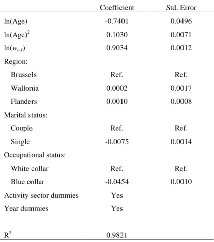
of heterogeneity, and is therefore preferred. In order to forecast wages, we used the observed earnings history for each individual in our sample and regressed the logarithm of the hourly wage of the individuals on the logarithm of the age and the logarithm of the age squared. Since the best predictor of this year's wage is last year's wage, we included the lagged wage rate. We also added dummies to control for the sector of activity given by NACE 2 digits, the occupational status, region of residence and marital status. Table 3 presents the wage forecasting equation. Wage forecasts were computed for all individuals up to the date of mandatory retirement using the coefficients of the regressions.
[Table 3 about here ]
4.3. Microsimulation models and benefits
Using the information contained in our data set, we were able to simulate the benefits entitlements (and disposable income) of individuals if they chose one of the three exit paths. This was done using a microsimulation model. MIMOSIS is a microsimulation model for the Belgian social security and personal income tax system, running on the administrative dataset described above. Since the data go back to the tax benefit year 2001, the legislation that is currently modeled as baseline legislation is the one of 20018.
For every age less than 65 in 2001, we simulated (up to the age of 65) the benefits the individuals were eligible for. Because of age, working history or occupational status, the individuals were not faced with the same opportunities. Using
MIMOSIS, we obtained for each age to come the benefits individuals could claim if they continued to work until that age.
As stated above, in order to take into account the stream of income individuals would receive after 65 we included the social security wealth (W). This is the present discounted value of all future benefit flows from a given social security scheme. Discounting was carried out allowing both for time preference and mortality adjustments. W was computed for every pathway towards retirement that the individual was eligible for.
8 For further details on MIMOSIS see
The W at 65 for a particular exit path of a worker of age a in the case of retirement at age h>a is therefore given by:
∑
= − = 100 65 ) ( ) ( s h s a h s B s W ϑ ρwhere θ(s) is the survival probability at age s (conditional on being alive at age a), ρ is the rate of time discount, and Bh(s) is the pension benefit expected at age s if the worker retires at age h.
Once we had obtained for each exit path the flow of net income (labor or pension income, net of social security contributions and personal income taxes, plus other benefits the household may be eligible for), we were able to derive, conditional on the observed behavior, the preference structure governing the retirement choice in the given institutional setting.
5. Estimation results
The model was estimated by maximum likelihood. The theoretical model requires additional assumptions in order to be estimated:
(i) The total number of hours of leisure (Li) available per week is bounded to 80 and the actual number of hours is obtained by subtracting the hours actually worked. Once retired, whatever the scheme, the number of hours of leisure is 80.
(ii) We assumed that each person is completely liquidity constrained. Benefits are treated as zero before the first eligibility age. This is not too far from the truth since virtually no one retires before some benefits are available.
(iii) As discussed before, the eligibility age in the conventional early retirement scheme may differ among individuals according to sectoral-level agreements. In our administrative dataset, we have this
information for each worker. Hence eligibility age varies between workers.
(iv) We introduced taste-shifters for income (X1) and leisure (X2).
Preferences for leisure may vary between individuals according to sex, age, being in a couple and the region of residence. There is no a priori
reason for not incorporating household characteristics into the utility of income. However recent studies on the utility of income derived from psychophysical literature assume that income is only influenced by the size of the household9.
(v) Finally, we performed a sensitivity analysis with respect to time preference and we retained a discount rate (ρ) of 3%, which is common in the literature.
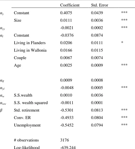
In Table 4, we present the results. The parameters in the utility function by themselves are not very informative. However, in order to be theoretically
consistent, the derivative with respect to income needs to be positive, which is the case. Concavity in income, in particular, is a required feature of the consistency of the model (Van Soest, 1995). The utility of wealth coming from a pension after 65 also displays diminishing returns. These results show that the size of the
household plays a positive role in the marginal utility of income. Being in a couple is insignificant. The age increases the marginal utility of leisure and thus increases the likelihood of retirement. Workers living in Flanders have higher utility from leisure. We note that the parameter associated with the interaction term between income and leisure is significantly different from zero and is negative. State dummies associated with the standard retirement, conventional early retirement and unemployment are all significant (continuing to work is the reference in this case).
[Table 4 about here]
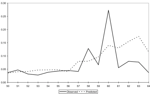
The results discussed so far seem satisfactory but we can also judge the prediction power of the model by comparing the observed and predicted probabilities of exiting the labor market. On average the model almost perfectly fits the data. The actual departure rate is 5.04% and the predicted departure rate is 5.46%. Figure 1 shows the probabilities of exit by age. The model barely fits the exit peaks
observed at 58 and 60. As discussed above, this finding is not new (see Stock and Wise,1990 and Samwick,1998). The model implies some persistence in individual preferences for working versus retirement. There may be an effect of the
"customary retirement age" with these ages of eligibility. In addition, the model
predicts rather well the probability of exit at other ages but overpredicts retirement after 61. It is difficult to find a clear reason for this difference. We can argue that the conventional early retirement scheme is the result of a multitude of sectoral agreements that each propose different eligibility rules. We have used the sectoral eligibility ages for this scheme but eligibility may occur later. In this context, our estimates offer many more opportunities to workers in comparison with what they actually face. Finally, as shown in Figure 2, the predicted cumulative hazard rates appear to be very close to the actual ones so that the model predicts accurately the cumulative exit behavior.
[Figure 1 about here] [Figure 2 about here]
6. Reforms simulations
Our model can be used to predict retirement behavior following a reform affecting the inter-temporal budget constraint. Such ex-ante analysis may give an insight into the potential impacts and serve as an evaluation tool to assess reforms aiming at increasing the employment rate of older people. To illustrate this, the effects of four alternative policy reforms are simulated:
(i) Policy 1: the first reform consists of reintroducing the standard
retirement scheme as it existed before 1991. Before that date, pensions taken anticipatively before 65, were penalized by a 5 % actuarial reduction of the benefits for each year of anticipation. Individuals taking their pension at 60, instead of 65, therefore received 75% (100% - 5x5%) of the benefit they would otherwise be entitled to.
(ii) Policy 2: the second reform consists simply of an increase by 3 years
of all key ages in the various schemes. After the reform, the first age of eligibility for claiming benefits in the standard retirement scheme is 63, it is 61 in the conventional early retirement scheme and for access to unemployment exempted from job search, it is 53.
(iii) Policy 3: the third reform consists of the so called "pension bonus".
Following the Belgian Intergenerational Solidarity Pact of 2005, employees working beyond the age of 62 can benefit from a pension supplement. The "bonus" of 2 EUR per day worked beyond these
limits increases the annual benefit payable, and this occurs
independently of the wage earned or the contributions accumulated.
(iv) Policy 4: the last reform consists of a policy that would equalize early
retirement schemes through a unique retirement age. From this reform, access to benefits is only possible at the age of 60 at the earliest, whatever the pathway.
The simulations are based on the estimates of Table 4. The baseline hazard rates are the model predictions under the 2001 system illustrated in the previous
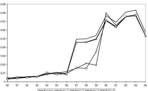
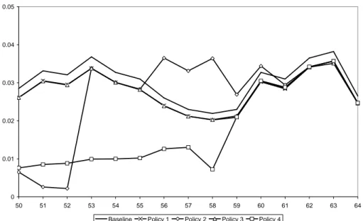
section. Figures 3 and 4 illustrate the hazard rates of departure and the cumulative distribution of departures under the different policies as compared to the baseline.
Policy 1: The introduction of a 5% actuarial reduction of the benefits in the
standard retirement system is expected to have a positive effect on labor supply between age 60 and 65. This reform should encourage additional work after age 60 through an income effect. We see on Figure 3 that the reform has a small negative effect on departures before 59 and a larger effect after 60. However such a reduction in benefits seems not to be sufficient to induce individuals to totally revising their exit choice since the average retirement age is marginally changed, as shown on Table 5. The change in the financial incentives seems to produce little impact on labor supply of older men.
[Table 5 about here]
Policy 2: This corresponds to an increase by 3 years of all the ages of eligibility.
The reform implies a drop in the departure rates. While the model predicts that almost 44% of those working at age 50 will leave before age 60, only 39% would have left if all eligibility ages had been increased by 3 years. We show on Figures A1, A2 and A3 in the appendix how this policy implies a drop in each exit path hazard rates before the new ages of eligibility. The exit rates through old-age unemployment fall largely before 53 and then increase faster than in the baseline. Before the age of 60, the exit rates of conventional early retirement are low. The fast increase in the exit rates at 57 vanishes and occurs now at 60. Finally the same kind of results applies for the standard retirement scheme where the peak occurs later. Interestingly, the effect of the reform on the effective age of
retirement is much stronger than in the previous simulation. Here it is 58.6 years old. This reflects the longer wait before the retirement benefits can be claimed.
Policy 3: The introduction of the pension bonus after 62 has a small impact.
Actually the pension bonus implies a higher social security wealth for every age of retirement after age 62. This should encourage additional work before age 62, but will reduce work among those already working past age 62 through an income effect. In Figures 3 and 4, the effect is similar to the effect of Policy 1 except after the age of 62. Interestingly, from 62 to 64, individuals use the standard retirement pathway (see Figure A 1) more often than they did before the reform. At the same time the number of retirees in the two other schemes decreases for these ages. The effect of the reform is a transfer of person from the early retirement scheme and the unemployment scheme to the standard retirement scheme. As a result, the average age of retirement does not change much.
Policy 4: Finally, we consider the last reform which consists of one set retirement
age at 60. The hazard rates drop considerably before the age of 60. Persons who are employed at 60 or older face the same options as before the reform. Looking at the cumulative distribution of departures, the model predicts that almost 44% of workers at age 50 will leave before the age of 60 under the baseline. Only 29% would leave if retirement had been at the age of 60 instead. This implies an increase in the effective retirement age to 59.3.
[Figure 3 about here] [Figure 4 about here]
These simulations are interesting on two points. First, social security certainly provides incentives for early retirement. But these incentives do not only result from a level of generosity in the amounts of benefits. The provision rules inherent in the social security systems are of great importance. Second, what emerge from these results is that there seems to be a real preference for retiring earlier in Belgium. Even if we reduce the generosity of provision, this has only a small impact on the behavior of workers. This is important at the time of reform of the systems. Only a mix of eligibility restriction with some reduction in financial incentives could achieve an increase in the labor force participation of older workers.
Finally, the results may appear rather small but we have to keep in mind that an increase of the retirement age of just 6 months would mean the avoidance of thousands of monthly benefits needing to be paid by social security. In the era of
an aging population and problems of financial sustainability for the social security program, this is not negligible. Our framework with the help of the
microsimulation MIMOSIS could also be applied to calculate the budgetary impact of these reforms but this is outside of the scope of this paper.
7. Conclusions
This paper develops a framework to model the retirement decisions of older workers. The model is forward looking and thus resembles the option value model. An individual compares the utility obtained under different choices of exit at different times. The proposed framework, however, extends the option value model in order to fully recover the structural preference parameters. We take into account the fact that the various paths to retirement preferences may vary between individuals through taste-shifters on income and leisure.
Based on administrative data for Belgium and with the help of the
microsimulation model MIMOSIS, we estimated the model parameters and used the estimation to assess four policy proposals for reforming the Belgian retirement system. Our simulations show that each reform might have an impact on
retirement rates but with variable success. Reforms that modify the access to every retirement pathway have more potential effects on the probability of exit than those simply targeting the generosity of the standard retirement scheme. However, we also show that the last reform implemented by the Belgian
government, the "pension bonus", does not seem to have the expected impact. On the contrary it could reduce the labor force participation before 65.
Acknowledgements
The authors thank the CrossRoads Banks of Social Security for the development of the ‘Datawarehouse labor market and social protection’ and John Dagsvik, André Decoster, Alain Jousten, Sergio Perelman, Pierre Pestieau and Arthur Van Soest for useful comments on the modelling strategy. Financial support from the “Communauté Française de Belgique” ARC contract (ARC 05/10-332) is gratefully acknowledged.
Appendix
Figure A1: Hazard rates by age – Wage-earners retirement system
0 0.01 0.02 0.03 0.04 0.05 0.06 50 51 52 53 54 55 56 57 58 59 60 61 62 63 64
Baseline Policy 1 Policy 2 Policy 3 Policy 4
Figure A2: Hazard rates by age – Conventional early retirement system
0 0.01 0.02 0.03 0.04 0.05 0.06 0.07 0.08 0.09 50 51 52 53 54 55 56 57 58 59 60 61 62 63 64
Figure A3: Hazard rates by age - Old-age unemployment system 0 0.01 0.02 0.03 0.04 0.05 50 51 52 53 54 55 56 57 58 59 60 61 62 63 64
Baseline Policy 1 Policy 2 Policy 3 Policy 4
Reference
Aaberge, R., U. Colombino, and S. Strom (2004) Do More Equal Slices Shrink the Cake? An Empirical Investigation of Tax-Transfer Reform Proposals in Italy. Journal of Population Economics, 17, 767-785.
Bargain, O., and K. Orsini (2006) In-Work Policies in Europe: Killing Two Birds with One Stone. Labour Economics, 13(6), 667-698.
Berkovec, J., and S. Stern (1991) Job Exit Behaviour of Older Men. Econometrica, 59, 189-210. Blundell, R., A. Duncan, J. McCrae, and C. Meghir (2000) The Labour Market impact of the Working Families Tax Credit, Fiscal Studies, 21, 75-104.
Coile, C., and J. Gruber (2001) Themes in the Economics of Aging, The University of Chicago Press, Chicago.
Coile, C., and J. Gruber (2007) Future Social Security Entitlements and the Retirement Decision, Review of Economics and Statistics, 89(2), 234-246.
Colombino, U. (2003) A simple Intertemporal Model of Retirement Estimated On Italian Cross-Section Data, Labour, 17, 115-137.
Dagsvik, J., and S. Strom (2004) Sectoral Labor Supply, Choice Restrictions and Functional Form, Statistics Norway Discussion Papers, No. 338.
Dagsvik, J., Jia, Z., Orsini, K. and G. Van Camp (2010) Subsidies on Low-skilled Workers’ Social Security Contributions: The Case of Belgium”, Empirical Economics, forthcoming.
Dellis, A., R. Desmet, A. Jousten, and S. Perelman (2004) Micro-modelling of Retirement in Belgium, in Social Security and Retirement Around the World: Micro-estimation, ed. by J. Gruber,
and D. Wise. University of Chicago Press, Chicago.
Feinstein, J., and D. McFadden (1989) The Dynamics of Housing Demand by the Elderly: Wealth, Cash Flow, and Demographic Effects, in The Economics of Aging, ed. by D. Wise. University of Chicago Press, Chicago.
Gustman, A., and T. Steinmeier (1986) A Structural Retirement Model, Econometrica, 54(3), 555-584.
Hausman, J., and D. Wise (1985) Social Security, Health Status and Retirement in Pensions, Labor and Individual Choice, ed. by D. Wise. University of Chicago Press, Chicago. Lumsdaine, R., J. Stock, and D. Wise (2001) Three Models of Retirement: Computational Complexity versus Predictive Validity in Topics in the Economics of Aging, ed. by D. Wise. The University of Chicago Press, Chicago.
McFadden, D. (1973) Conditional Logit Analysis of Qualitative Choice Behavior in Frontiers in Econometrics, ed. by P. Zarembka. Academic Press, New York.
Pestieau, P., and J. Stijns (1999) Social Security and Retirement in Belgium in Social Security and Retirement Around the World: Micro-estimation, ed. by J. Gruber, and D. Wise. University of Chicago Press, Chicago.
Samwick, A. (1998) New Evidence on Pensions, Social Security, and the Timing of Retirement, Journal of Public Economics, 70, 207-236.
Stock, J., and D. Wise (1990) Pensions, the Option Value of Work, and Retirement, Econometrica, 58, 1151-1180.
Van Soest, A. (1995) Structural Models of Family Labor Supply: A Discrete Choice Approach, Journal of Human Resources, 30, 63-88.
Van Soest, A., M. Das, and X. Gong (2002) A Structural Labour Supply Model with Flexible Preferences, Journal of Econometrics, 107, 345-374.
Figure 1 : Hazard rates by age
0.00 0.05 0.10 0.15 0.20 0.25 0.30 50 51 52 53 54 55 56 57 58 59 60 61 62 63 64 Observed Predicted
Figure 2 : Cumulative hazard rates by age
0.0 0.2 0.4 0.6 0.8 1.0 50 51 52 53 54 55 56 57 58 59 60 61 62 63 64 Observed Predicted
Figure 3 : Simulations – Hazard rates by age 0.00 0.05 0.10 0.15 0.20 50 51 52 53 54 55 56 57 58 59 60 61 62 63 64
Baseline Policy 1 Policy 2 Policy 3 Policy 4
Figure 4 : Simulations – Cumulative hazard rates by age
0.0 0.2 0.4 0.6 0.8 1.0 50 51 52 53 54 55 56 57 58 59 60 61 62 63 64
Baseline Policy 1 Policy 2 Policy 3 Policy 4
Table 1 : Exit schemes in 2001 Old-age unemployment Conventional early retirement Wage-earners retirement All schemes Number of people 155,921 114,930 182,653 453,504 % 34% 25% 40% 100% Eligibility Age 50 58 60
Career 20 years 25 years
+ 624 days
No restriction
Table 2 : Sample statistics N 3176 Household size 2.7 Age 54 Living in couple 90.5% Living in Wallonia 29.4% Living in Flanders 63.2% Yearly net wage (in€) 25,743 Length of career (in years) 35
% of exit by age 50 3.7% 51 4.7% 52 3.2% 53 2.8% 54 3.8% 55 4.3% 56 4.5% 57 4.1% 58 12.8% 59 6.6% 60 27.4% 61 5.5% 62 8.0% 63 7.7% 64 3.7%
Source: Datawarehouse Labor Market and Social Protection
Table 3 : Wage forecasting equation Dependent variable : ln(wt) Coefficient Std. Error ln(Age) -0.7401 0.0496 ln(Age)2 0.1030 0.0071 ln(wt-1) 0.9034 0.0012 Region:
Brussels Ref. Ref.
Wallonia 0.0002 0.0017
Flanders 0.0010 0.0008
Marital status:
Couple Ref. Ref.
Single -0.0075 0.0014
Occupational status:
White collar Ref. Ref.
Blue collar -0.0454 0.0010
Activity sector dummies Yes
Year dummies Yes
Table 4 : Parameters estimates Coefficient Std. Error αy Constant 0.4075 0.0439 *** Size 0.0111 0.0036 *** αyy -0.0021 0.0002 *** αl Constant -0.0376 0.0874 Living in Flanders 0.0206 0.0111 * Living in Wallonia 0.0166 0.0115 Couple 0.0067 0.0074 Age 0.0025 0.0009 *** αll 0.0009 0.0008 αyl -0.0048 0.0005 *** αw S.S.wealth 0.0010 0.0036 αww S.S. wealth squared -0.0011 0.0001 β Std. retirement -0.5301 0.0813 *** Conv. ER -0.4933 0.0804 *** Unemployment -0.5452 0.0794 *** # observations 3176 Log-likelihood -639.244
Note: The amount of income is divided by 1000 and the amount of S.S. wealth is divided by 10000.
Table 5 : Average retirement age
Baseline Policy 1 Policy 2 Policy 3 Policy 4
Average