Structural damage detection based on PCA of vibration measurements

STRUCTURAL DAMAGE DETECTION BASED ON PRINCIPAL COMPONENT ANALYSIS OF VIBRATION MEASUREMENTS

J.-C. Golinval, P. De Boe, A.-M. Yan, G. Kerschen University of Liege

Département AéroSpatiale Mécanique et MAtériaux (ASMA) LTAS – Vibrations et Identification des Structures,

Chemin des chevreuils, 1, Bât. B52 B-4000 Liège, Belgium.

Phone: +32 4 366 48 53 Fax : +32 4 366 48 56 E-mail: [email protected]

Abstract: This paper deals with the application of statistical process control techniques based on principal component analysis to vibration-based damage diagnosis of structures. Principal component analysis of the sensor time-responses allows to extract principal directions (i.e. features) which define a subspace that is representative of the dynamics of the instrumented structure. Any change in the response of a single sensor will affect the subspace spanned by the complete sensor response set. It follows that the subspace corresponding to the current state of the structure can be compared to the subspace of the initial state of the structure, assumed to be healthy, in order to diagnose possible damage. Principal component analysis may also be performed for every potential subset of damaged sensors in order to identify the involved sensor, and, therefore, the damaged substructure. In this paper, the problem of structural damage detection is addressed in the case of environmental vibration testing. A direct application is presented for a test item submitted to random vibration testing by means of an electro-dynamic shaker.

Key Words: Damage detection; Principal component analysis; Structural health monitoring; Vibration testing;

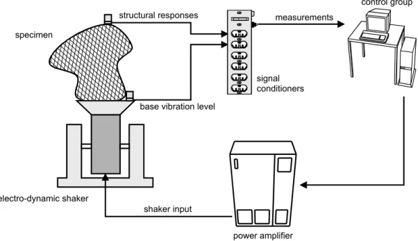
Introduction: Mechanical equipments in operational use are subjected to various excitations that may result in significant vibration levels and consequently may cause structural damages and/or fatigue failures. In order to ensure that the equipment is able to withstand its dynamic environment, fatigue testing is often performed using vibration exciters. Fig. 1 gives the general layout of an electro-dynamic vibration exciter system showing the test item instrumented with accelerometers, the acquisition system, the controller and the power amplifier, which drives the vibration exciter. The acceleration measured at the driving point is used by the controller as a feedback to ensure the prescribed vibration level.

specimen

electro-dynamic shaker

power amplifier

control group structural responses

base vibration level

measurements

shaker input

signal conditioners

Figure 1. Typical set-up for vibration testing

Depending on vibration standards, the test item may be submitted to different kinds of excitation signals e.g. sine sweep, sine dwell, random, shock, etc. Classically, structural damages are identified by visual inspection and/or by comparing frequency spectra at chosen locations before and after the test. In practice, this methodology may present drawbacks such as the difficulty to manage a large amount of data and the fact that spectra comparison are only performed after the test. It follows that vibration qualification tests are usually time-consuming.

The goal of this paper is to propose a damage detection method that may be used during the test duration to check the structural integrity of the test item. The proposed method is based on the principal component analysis (PCA) of the vibration signals. PCA, also known as Karhunen-Loève decomposition or Proper Orthogonal Decomposition (POD), is a multi-variate statistical technique that has been first used in the mechanics community by Lumley [1]. It has also been used recently for several purposes including model reduction [2], dynamic characterization [3], sensor validation [4], modal analysis [5], parameter identification [6] or damage detection [7].

It is important to note that the proposed method does not require the knowledge of the excitation.

Principal Component Analysis of Vibration Data: Let us consider a mechanical structure instrumented by nS sensors, e.g. vibration transducers (accelerometers,

displacement and velocity transducers), strain gauges, temperature sensors, etc. The measured data (a snapshot) are collected in a vector q and are supposed to be gathered at

b instants. Accordingly, the observation matrix Q of dimension nS × b (with b >> nS) is formed:

( )

( )

( )

( )

( )

( )

When various transducers are used and when the measured variables are of different kind (displacement, velocity, acceleration, pressure, temperature, etc), a data normalization procedure is usually required to lead to normalized variables with zero-mean and unitary standard deviation.

( )

( )

where q ,n σn are the mean value and the standard deviation of each data set measured at

sensor n respectively, i.e.

( )

( )

∑

∑

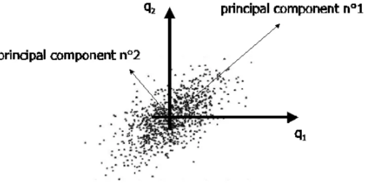
PCA of measurement data allows to seek for a linear mapping of the high-dimensional data to a lower dimensional space. The first principal direction corresponds to the optimal vector (in a least square sense) to characterize the ensemble of snapshots. The second principal direction is the optimal vector to characterize the ensemble of snapshots but restricted to the space orthogonal to the first principal direction, and so forth. Fig. 2 illustrates the principle of the method in the case of two sensors (nS=2).

The singular value decomposition (SVD) constitutes an effective way of calculating the principal components of the observation matrix Q.

(4) T

Q = U Σ V

where U is an orthonormal matrix (nS × nS); its columns form the hyperplane spanned by

the principal directions in which lie all the observations q(tj). Σ is an (nS × b)

pseudo-diagonal and semi-positive definite matrix with pseudo-diagonal entries containing the singular values, sorted in descending order. V is an (b × b) orthonormal matrix whose each column contains the time modulation of the corresponding principal direction. The SVD of the observation matrix, seen as a collection of column vectors (or snapshots), provides important insight into the oriented energy distribution of this set of vectors. Roughly speaking, each singular value represents the relative importance of the associated principal direction in the dynamic response of the structure. In other words, it means that the structural motions will preferentially be directed according to the principal directions related to the greatest singular values. It follows that the lowest singular values, which are related to noise effects, may be discarded.

In most cases, the number of measurement samples may be very large (b >>) so that the principal directions are most easily computed as the eigenvectors of the covariance matrix Q QT: (5) T 2 Q Q = U Σ UT r α u

Structural damage detection: The observation matrix Q may be expressed in terms of mode-shape vectors in the form:

(6)

( )

(

)

( )

∑

where m is the number of modes Φ(i) in the frequency band of interest; S is the sensor

influence matrix, R is the residual vector associated with the modes located outside the frequency band and αi (t), αr (t) are modal coordinates.

On the other hand, equation (4) may be rewritten in the form:

(7) ( ) nS T i i i 1 ( t ) β = = =

∑

where u(i) is the ith principal direction (column of matrix U) and βi (t) is a time-dependent

coefficient.

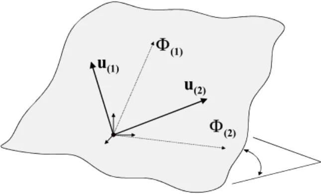
The comparison between equations (6) and (7) shows that the subspace (or hyperplane) covered by the principal directions u(i) is identical to the invariant subspace covered by

the modes Φ(i). Geometrically speaking, we observe that the principal directions extracted

mode-shape vectors, as shown in Fig. 3 in the two-dimensional case. Mathematically speaking, it means that the hyperplane spanned by the principal directions of the observation matrix is an invariant feature of the structure, even if the directions of the principal vectors are dependent on the excitation. This invariance property renders the PCA of the observation matrix useful for structural damage detection. The key idea of the method is to compare the hyperplanes associated respectively with the reference (undamaged) state of the structure and with the current (potentially damaged) state of the structure.

One way to compare hyperplanes is to use the concept of angles between two subspaces as illustrated in Fig. 3 in the two-dimensional case. This concept, introduced by Jordan [8] allows to quantify the spatial coherence between two time-history blocks of an oscillating system. Let A∈

ℜ

ℜ

ℜ

ℜ

Thus, the singular values of QT_AQ_B define q cosines of the principal angles θi between

A and B:

(9)

(

)

(

( )

)

(

i

SVD Q Q_{A B} → diag cos θ i 1,= …, q

)

It follows that the largest angle may be used as an indicator to quantify how much the subspaces defined by the columns of matrices A and B are globally different.

Φ₍₁₎

Φ₍₂₎ u₍₁₎

u₍₂₎

Fig. 3. The principal components and the concept of angle between subspaces

Damage localization: Once damage has been detected using the concept of angles between the reference and the current hyperplanes the idea pursued here for its localization is to identify which sensor set mostly affects the current hyperplane (corresponding to the damaged state). For this purpose, sensors are separated into two groups: the assumed “damaged” set and the undamaged one. It is assumed here that a

small damage localized in a substructure is not responsible for a significant change in the dynamics of the whole structure but significantly affects the response of the involved substructure, so that the subspace spanned by the undamaged sensors will not exhibit appreciable differences between the reference and the damaged states. In that case, the identification of the damaged substructure may be performed by computing the subspace angle between the pre- and post-damaged states; it follows that the angle remains small when the sensors located on the damaged substructure are removed from the working sensor subset.

(a) (b)

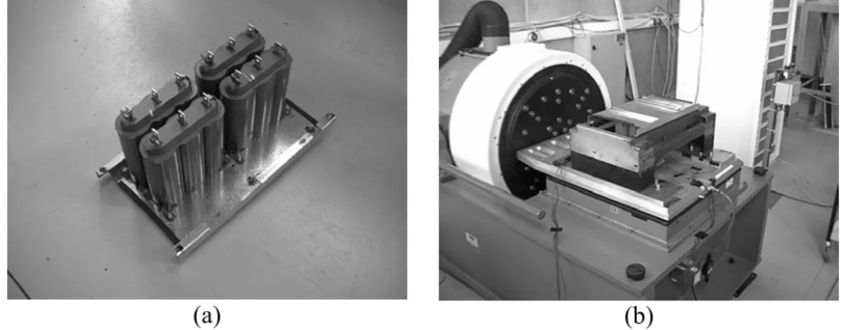
Fig. 4. (a) Assembly of capacitors (b) mounted on the electro-dynamic exciter

Vibration testing of capacitors: The test item considered here consists of an assembly of electrical capacitors mounted fixed on an interface plate as shown in Fig. 4.(a). The capacitor assembly is mounted on the slip-table of the electro-dynamic shaker (26.6 kN) as illustrated in Fig. 4.(b). The test specifications consist in a random excitation of magnitude 2.5 gRMS in the [5-200 Hz] frequency range and the total test duration is ten minutes. Each capacitor is instrumented with an accelerometer. During the test, a crack is initiated at the fixation of one of the capacitors and the fixation breaks after a few minutes as shown in Fig. 5.

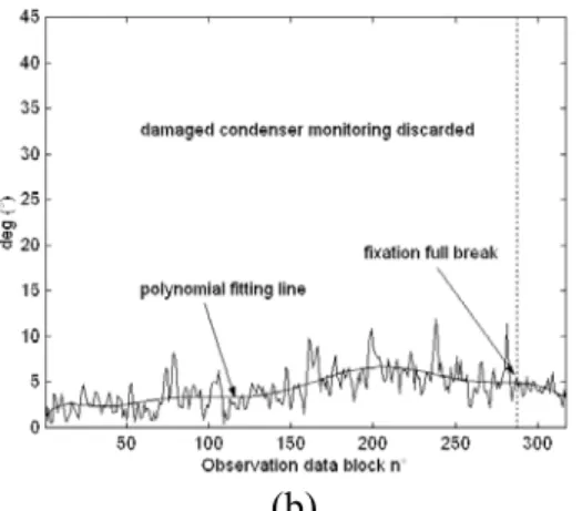
For the purpose of damage detection, the principal component analysis was performed on the whole set of accelerometers using overlapped windows of 4 seconds. For each data block acquisition, the hyperplane corresponding to the current state of the structure was compared with the hyperplane corresponding to the reference (undamaged) state of the structure using the concept of angles between subspaces. The results are shown in Fig. 6. (a) where the time evolution of the angle is depicted. Note that the damage detection criterion based on the angle between subspaces clearly indicates the damage evolution in the capacitor assembly. It can also be observed in Fig. 6. (b) that the angle deviation remains low when the data corresponding to the sensors mounted on the damaged capacitor are not included in the observation matrix.

(a) (b)

Fig. 6. (a) Detection of the damage (b) Localization of the damage

Conclusion: The goal of this paper was to present a damage detection method based on the principal component analysis of vibration measurements and on the concept of angle between subspaces. The method was illustrated in the case of fatigue vibration testing using an electro-dynamic shaker but it may generalized to many other applications in the field of structural health monitoring. It has been shown that the proposed method is able to detect the apparition of a crack and to follow the evolution of the structural failure. The proposed procedure is very easy to implement and remains computationally cheap. Therefore, it looks very promising for on-line monitoring implementation. When fatigue testing of mechanical structure is to be performed, it would enable the test operator to decide to abort or to complete the test.

Acknowledgements: This work is supported by a grant from the Walloon government as a part of the convention n°9613419. The author G. Kerschen is supported by a grant from the Belgian National Fund for Scientific Research (FNRS) which is gratefully acknowledged.

References

[1] Lumley, J. (1970). “Stochastic Tools In Turbulence”, New York: Academic Press. [2] Azeez, M.F.A., Vakakis, A.F. (1998). “Proper Orthogonal Decomposition of a Class

of Vibroimpact Oscillations, Journal of Sound and Vibration, 240: 859-889.

[3] Kappagantu, R., Feeny, B.F. (2000). “Part 1: Dynamical Characterization of a Frictionally Excited Beam”, Nonlinear Dynamics, 22: 317-333.

[4] Friswell, M. I. and Inman, D. J. (1999). “Sensor Validation for Smart Structures,” Journal of Intelligent Material Systems and Structures, 10: 973-982.

[5] Han, S., Feeny, B.F. (2003). “Application of Proper Orthogonal Decomposition to Structural Vibration Analysis”, Mechanical Systems and Signal Processing, 17: 989-1001.

[6] Lenaerts, V., Kerschen, G., Golinval, J.-C. (2001). “Proper Orthogonal Decomposition for Model Updating of Non-Linear Mechanical Systems," Mechanical Systems and Signal Processing, 15(1): 31-43.

[7] De Boe P., Golinval, J.-C. (2003). “Principal component analysis of piezo-sensor array for damage localization" Structural Health Monitoring: An International Journal, 2(2): 137-144.

[8] Jordan, C. (1875), “Essai sur la géométrie à n dimensions“, Bulletin de la Société mathématique, 3 : 103-174.