Supervised detection of exoplanets in high-contrast imaging sequences

Astronomy

_&

Astrophysics

© ESO 2018

Supervised detection of exoplanets in high-contrast

imaging sequences

C. A. Gomez Gonzalez

_{, O. Absil}

_{, and M. Van Droogenbroeck}

1_{STAR Institute, Université de Liège, Allée du Six Août 19C, 4000 Liège, Belgium} 2_{Université Grenoble Alpes, IPAG, 38000 Grenoble, France}

3_{Montefiore Institute, Université de Liège, 4000 Liège, Belgium}

Received 17 September 2017 / Accepted 12 December 2017

ABSTRACT

Context. Post-processing algorithms play a key role in pushing the detection limits of high-contrast imaging (HCI) instruments. State-of-the-art image processing approaches for HCI enable the production of science-ready images relying on unsupervised learning techniques, such as low-rank approximations, for generating a model point spread function (PSF) and subtracting the residual starlight and speckle noise.

Aims. In order to maximize the detection rate of HCI instruments and survey campaigns, advanced algorithms with higher sensitivities to faint companions are needed, especially for the speckle-dominated innermost region of the images.

Methods. We propose a reformulation of the exoplanet detection task (for ADI sequences) that builds on well-established machine learning techniques to take HCI post-processing from an unsupervised to a supervised learning context. In this new framework, we present algorithmic solutions using two different discriminative models: SODIRF (random forests) and SODINN (neural networks). We test these algorithms on real ADI datasets from VLT/NACO and VLT/SPHERE HCI instruments. We then assess their performances by injecting fake companions and using receiver operating characteristic analysis. This is done in comparison with state-of-the-art ADI algorithms, such as ADI principal component analysis (ADI-PCA).

Results. This study shows the improved sensitivity versus specificity trade-off of the proposed supervised detection approach. At the diffraction limit, SODINN improves the true positive rate by a factor ranging from ∼2 to ∼10 (depending on the dataset and angular separation) with respect to ADI-PCA when working at the same false-positive level.

Conclusions. The proposed supervised detection framework outperforms state-of-the-art techniques in the task of discriminating planet signal from speckles. In addition, it offers the possibility of re-processing existing HCI databases to maximize their scientific return and potentially improve the demographics of directly imaged exoplanets.

Key words. methods: data analysis – techniques: high angular resolution – techniques: imaging spectroscopy – planetary systems – planets and satellites: detection

1. Introduction

In the last decade, direct imaging of exoplanets has become a reality thanks to advances in optimized wavefront control (for a review see Milli et al. 2016), specialized coronagraphs (Rouan et al. 2000; Spergel & Kasdin 2001; Soummer 2005;

Mawet et al. 2005; Kenworthy et al. 2007), innovative observ-ing techniques (Sparks & Ford 2002; Marois et al. 2006) and dedicated post-processing algorithms (Lafrenière et al. 2007;

Mugnier et al. 2009; Amara & Quanz 2012; Soummer et al. 2012;Gomez Gonzalez et al. 2016). Direct observations of exo-planets provide a powerful complement to indirect detection techniques. They enable the exploration (thanks to their high sensitivity to wide orbits) of different regions of the parameter space, the study of planetary system dynamics, and photometric and spectroscopic characterization of companions. The con-sensus, after more than ten years of high-contrast imaging, is that massive planets, such as those of HR8799 (Marois et al. 2008, 2010), are rare at wide separations. A meta-analysis of 384 stars conducted by Bowler (2016) concluded that about 1% of them1 _{have giant planets at separations between 10 and}

?

F.R.S.-FNRS Research Associate.

1 _0.8+1.0

−0.6% occurrence rate.

1000 AU. On the other hand, from indirect methods, we know that super-Earths and rocky planets are much more common than giant planets. For this reason, the development of new image-processing techniques is of key importance for maximiz-ing the scientific return of existmaximiz-ing first- and second-generation high-contrast imaging (HCI) instruments, especially at small separations from the host star. Indeed, the amount of avail-able archival HCI data has increased rapidly with the advent of second-generation instruments, such as the Spectro-Polarimetric High-contrast Exoplanet REsearch (VLT/SPHERE;Beuzit et al. 2008) and Gemini Planet Imager (GPI; Graham et al. 2007). However, the adoption of the latest developments in data man-agement and machine learning in the HCI community has been slow compared to fields such as computer vision, biology, and medical sciences.

Increases in computational power and data storage in the last decade have enabled the emergence of data-driven discov-ery methods in sciences (Ball & Brunner 2010), in parallel to the popularization of machine learning and data science fields of study. Data-driven models are especially important in HCI, if we consider the sheer amount of data that mod-ern high-contrast imaging instruments are producing. Machine learning techniques have proven to be useful in a variety of

astronomical applications over the last decade. Artificial neural networks are an algorithmic approach proposed a few decades ago in the machine learning community, inspired by our under-standing of the biology and structure of the brain. Only recently, with graphics processing unit (GPU) computing going main-stream, larger amounts of data, and the use of deep architectures (with increased number of layers and neurons), deep learn-ing has led to breakthroughs in the most challenglearn-ing areas of machine learning (Goodfellow et al. 2016). In particular, it has produced impressive results in fields dealing with percep-tual data, such as computer vision and language understanding, removing the necessity of hand-crafted features (Xie et al. 2017). Although neural networks have been used in astronomy since the early nineties (Odewahn et al. 1992;Bertin & Arnouts 1996;

Tagliaferri et al. 2003), the use of deep learning has started to spread only in the last couple of years. Convolutional neu-ral networks (CNN;LeCun et al. 1989;Krizhevsky et al. 2012) are becoming more and more common for image-related tasks, such as galaxy morphology prediction (Dieleman et al. 2015), astronomical image reconstruction (Flamary 2016), photometric redshift prediction (Hoyle 2016), and star-galaxy classification (Kim & Brunner 2017). Other deep neural network architectures, such as autoencoders and generative adversarial networks, have been used for feature-learning in spectral energy distributions of galaxies (Frontera-Pons et al. 2017) and for image reconstruc-tion as an alternative to convenreconstruc-tional deconvolureconstruc-tion techniques (Schawinski et al. 2017).

A typical HCI planet hunter pipeline includes the produc-tion of a science-ready final image, where potential exoplanets are flagged by visual inspection aided by the computation of a signal-to-noise (S/N) metric. In this study, we adopt the S/N definition ofMawet et al.(2014) which addresses the small sam-ple statistics effect at small separations. In the case of angular differential imaging (ADI; Marois et al. 2006) data, the gen-eration of a final image usually relies on differential imaging post-processing techniques. In this study, we present a refor-mulation of the exoplanet detection task as a supervised binary classification problem.

This paper is organized as follows. In Sect. 2 we briefly review the state-of-the-art image processing techniques for HCI and present a novel supervised framework for exoplanet detec-tion. In Sect.3, we describe our labeled data-generation strategy for ADI datasets. Section 4 describes the two proposed clas-sification approaches using random forests and deep neural networks. Section5explains the prediction stage of our super-vised detection framework. Section 6 presents a performance assessment study using signal detection metrics for compar-ing our supervised detection approach to state-of-the-art HCI algorithms, and Sect.7presents our conclusions.

2. From unsupervised to supervised learning The purpose of differential imaging post-processing techniques is to reduce the image dynamic range, by modeling and subtract-ing the contribution from the high-flux pixels belongsubtract-ing to the residual starlight and from the quasi-static speckle noise. This procedure, also called model point spread function (PSF) sub-traction, produces residual final images where, unfortunately, part of the companion signal is lost due to it being fitted in the model PSF (companion self-subtraction). Here we define the model PSF as the algorithmically built image that we use with differential imaging techniques for subtracting the scattered starlight and speckle noise pattern in order to enhance the signal of disks and exoplanets. Among the model PSF subtraction

techniques, we count LOCI (Lafrenière et al. 2007), principal component analysis (PCA)-based algorithms (Soummer et al. 2012;Amara & Quanz 2012), and LLSG (Gomez Gonzalez et al. 2016). All these approaches use different types of low-rank approximation to generate a model PSF. A different approach is taken by ANDROMEDA (Mugnier et al. 2009;Cantalloube et al. 2015), which employs maximum likelihood estimation on residual images obtained by pairwise subtraction within the ADI sequence.

The exoplanet detection problem is critical as it triggers all subsequent steps, such as the determination of position, flux, and other astrophysical parameters (characterization) of potential companions. The task of detecting potential compan-ions with model PSF subtraction techniques lacks automation. It boils down to the visual identification of patches of pix-els sharing the same properties, such as bright regions on the images, and resembling the instrumental PSF. Therefore, the detectability of significant blobs by visual inspection is limited by human perception biases. This process is aided by the compu-tation of the S/N metric, but computing S/N maps is ultimately upper bounded by the performance of the chosen model PSF-subtraction technique. Moreover, the S/N metric does not deal with the truthfulness of potential companions. Other approaches to detecting blobs such as the Laplacian of Gaussian and the matched filtering (Ruffio et al. 2017) suffer from the same problem. For a review of general-purpose source-detection tech-niques on astronomical images, seeMasias et al.(2012).

Advanced approaches with higher sensitivities to dim com-panions are needed, especially for the speckle-dominated inner-most region of the images. Such approaches must address the issues of the visual vetting and S/N map computations by producing per-pixel likelihoods or probabilities of companion presence for a given ADI sequence. The maximum likelihood approach of ANDROMEDA, while a step in this direction, has not been thoroughly benchmarked against state-of-the-art approaches. Comparative contrast curves show its performance to be at the same level as full-frame ADI-PCA (Cantalloube et al. 2015).

A different approach to detecting exoplanets through HCI is the use of discriminative models, as has been proposed byFergus et al.(2014) for the case of multiple-channel SDI data. The DS4 algorithm, an extension of the S4 algorithm, adopts a discrim-inative approach based on support vector machines trained on a labeled dataset. This dataset is composed of negative samples taken directly from the input data and positive samples gener-ated by injecting synthetic companions. Unfortunately, there is no publication describing the details of this algorithm or robustly assessing its performance (see the discussion section ofFergus et al. 2014).

Differential imaging post-processing approaches rely on unsupervised learning techniques, such as low-rank approxima-tions, to enable the production of final residual images. The detection ability of these techniques depends on a variety of factors, including the number of frames in the sequence, the total range of field rotation, the distance of a companion to its parent star, the companion flux with respect to the star, and the aggressiveness of the differential imaging subtraction approach.

Supervised detection of exoplanets through HCI

Our approach here consists in a reformulation of the exoplanet detection task as a supervised binary classification problem. Supervised learning uses a considerable amount of labeled data

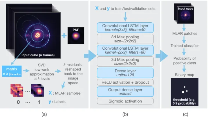
Fig. 1.The three stages of our supervised detection framework. Panel a: labeled data generation step. The ADI sequence and off-axis PSF template are examples of VLT/SPHERE data. Panel b: model training step for the case of SODINN. SODIRF uses a random forest classifier instead of a deep neural network. Panel c: evaluation of the trained model on the original cube and shows the schematic representation of the output detection map.

(or ground truth) in order to train a discriminative model and produce predictions. Depending on the model used, two algo-rithms are proposed: SODIRF, which stands for Supervised exOplanet detection via Direct Imaging with Random Forests, and SODINN, which stands for Supervised exOplanet detection via Direct Imaging with deep Neural Networks.

The first stage of our method addresses the challenge of gen-erating a large labeled dataset from a single ADI image sequence. As we show in Sect. 3 this procedure relies on the injection of synthetic companions and a technique called data augmen-tation, which is widely used in deep learning. Once our model is trained on this labeled dataset, it can be applied to the input ADI sequence for evaluation without risk of overfitting. Model overfitting occurs when a machine learning algorithm models random noise in the labeled training data, limiting the prediction power on unseen new data (lack of generalization). For high-capacity models, such as deep neural networks, overfitting also occurs when the model memorizes the labeled training data lim-iting the prediction ability on new data samples. Figure1shows a diagram of our novel framework for the case of SODINN.

The fact that SODIRF and SODINN can be trained on a labeled dataset created from a given ADI sequence means that these models are fine-tuned to each ADI sequence (Braham & Van Droogenbroeck 2016). We have tested SODIRF and SODINN on coronagraphic ADI sequences from different instruments. To validate our results, we focus on two datasets (one of them with a known companion) that are very different in terms of their characteristics. The first dataset, an L0 _band

VLT/NACO sequence on β Pic (Absil et al. 2013) and its com-panion (Lagrange et al. 2010), consists of 612 frames with 8 s of effective integration time, and has a total field rotation of 83 degrees. This β Pic dataset is described inAbsil et al.(2013) along with the pre-processing procedures applied to generate the

calibrated cube (or reduced image sequence) that we used here. The second dataset is a VLT/SPHERE sequence on V471 Tau (Hardy et al. 2015) acquired with the Infra-Red Dual-band Imag-ing and Spectroscopy (IRDIS; Dohlen et al. 2008) subsystem. The SPHERE/IRDIS instrument provides dual-band imaging thanks to the use of a beam splitter located downstream the coro-nagraphic mask. It consists of two sequences (in the H2 and H3 bands) with 50 frames, each one with 64 s of integration time, and a total field rotation of 30 degrees. The pre-processing steps applied to the V471 Tau dataset are described in Hardy et al.

(2015). Throughout this study, and for simplicity, we assume that

(1×)FWHM= 1λ/D = 4 pxs.

3. Generation of a labeled dataset

The generation of a labeled dataset requires a transformation of the ADI image sequence that better suits a supervised learning problem and enables us to create examples of two distinguishable classes: one representing the companion signal and the other the speckles and background areas. Therefore, we work on patches, instead of full frames, in order to get a different view of the image sequence. This choice is motivated by the fact that the exoplanet’s signal spatial scale is small compared to the frame size, and that it facilitates the creation of a large labeled dataset even from a single ADI sequence, as explained hereafter.

Working with two-dimensional (2D) patches directly from a pre-processed ADI sequence does not facilitate the genera-tion of two distinguishable classes. This is mainly due to the high dynamic range caused by the presence of residual starlight. Our initial tests using 2D patches were not successful and this motivated the use of a different view of the data. Our labeled dataset is composed of three-dimensional (3D) residual patches, at several Singular Value Decomposition (SVD) approximation

Fig. 2.Generation of a labeled dataset. Left panel: procedure for deter-mining the approximation levels and shows the cumulative explained variance ratio as defined by Eq. (4). The vertical dotted line is located at the maximum number (16) of singular vectors used in this case. Right panel: determination of flux intervals and shows the median S/N of injected companions, in an ADI-median-subtracted residual frame, as a function of the scaling factor. The red dots denote the lower and upper bounds of the companion injections for generating MLAR samples of the positive class.

levels, hereafter referred to as Multi-level Low-rank Approxi-mation Residual (MLAR) samples. They can be understood as computing annulus-wise PCA residual patches at different num-bers of principal components (PC). Working with these MLAR patches, we replace the ADI temporal information with the patch evolution as a function of the approximation level.

The MLAR samples are built in the following way. Consid-ering a matrix M ∈ Rn×p whose rows contain the pixels inside a centered annulus of a given width, n is the number of frames in the ADI sequence and p is the number of pixels in the given annulus. We reiterate that singular value decomposition (SVD) is a matrix factorization such that:

M= UΣVT=

n

X

i=1

σiuivTi, (1)

where the vectors ui and vi are the left and right singular

vec-tors, and σi the singular values of M. SVD is involved in

several least-squares problems, such as finding the best low-rank approximation of M in the least-squares sense, that is,

argmin

X

kM − Xk2_F, (2)

where k·k2_F denotes the Frobenius norm. By keeping k right singular vectors, we form a low-dimensional subspace B cap-turing most of the variance of M. The residuals are obtained by subtracting from M its projection onto B:

R= M − MBTB. (3)

This residual matrix is later reshaped to the image space, de-rotated and median combined as the usual ADI workflow dictates. In general, the larger the value of k, the better the reconstruction and the smaller the residuals (with less energy or standard deviation).

Instead of choosing one single k value for estimating the low-rank approximation of M and obtaining a single residual flux image (which is the goal of PCA-based approaches), we choose multiple k values sampling different levels of reconstruction. The MLAR patches are obtained by cropping square patches

of odd size, and about twice the size of the FWHM, from the sequence of final residual frames obtained for different k. Defin-ing the values of k relies on the cumulative explained variance ratio (CEVR). Let ˆMbe the matrix M, from which its temporal mean has been subtracted, and ˆσithe singular values of ˆM. The

explained variance ratio for the kth singular vector is defined as: ( ˆσk2/n)

P

iσˆi2

, (4)

where i goes from one to min(n, p). It measures the variance explained by each singular vector and the CEVR measures the cumulative explained variance up to the kth singular vector. Sen-sible values for k lie within the interval from 0.5 to 0.99 CEVR (for one example, see left panel in Fig.2), but depend on each particular dataset. The number of steps in this interval can be tuned, although the general rule is that more steps in the MLAR patches lead to more expressive samples that generally lead to higher classification power and a better discriminative model. In our tests, with 8 to 20 approximation levels, we could train models with outstanding accuracy.

By using this data transformation, we are able to generate MLAR samples from our two classes, one containing the signa-ture of a companion (positive class c+) and the other representing the background and speckle diversity (negative class c−). Each sample has an associated label y ∈ {c−_{, c}+_}.

3.1. Generation of the C+MLAR samples

The creation of the positive class relies on injecting an off-axis PSF template, a procedure accepted within the HCI community for generating synthetic data and assessing the sensitivity lim-its of image-processing algorithms and instruments. The PSF template is usually obtained from observations of the same star during the same observing run and without a coronagraph. The injection consists in the addition of such a PSF template (on each frame of the sequence) at a given location with a ran-dom brightness from a predefined interval. This interval must be carefully chosen to avoid class overlap, which occurs when the same MLAR sample (or very similar) appears as a valid example of both classes. This can happen when the lower bound of our brightness interval (or planet-to-star contrast) is too low, in which case the signature of the companion signal is hardly distinguishable from the one of the background polluted with quasi-static speckles. Sensible lower and upper bounds can be estimated in a data-driven fashion by injecting fake companions and measuring their S/N in residual frames obtained through classical ADI median subtraction. Fluxes leading to S/Ns in the interval [1,3] are usually good for our purpose (see right panel in Fig.2). These flux intervals are defined in an annulus-wise fashion and are therefore related to the radial flux profile of the images.

3.2. Generation of the C−_{MLAR samples}

The generation of the samples from the negative class, represent-ing everythrepresent-ing but the signal of companions (the background and speckles), relies on the exploitation of the rotation asso-ciated to an ADI sequence and common machine learning data-augmentation techniques2_{. The generation of a large}

num-ber of negative samples faces two main difficulties. First, the fact

2 _{This refers to the process of creating synthetic data and adding these}

to the training set in order to make a machine learning model generalize better (see Sect. 7.4 ofGoodfellow et al. 2016).

Fig. 3.MLAR samples from the positive and negative classes obtained with up to 16 singular vectors. The CEVR for these MLAR samples are shown in Fig.2. Panel a: each row corresponds to a random MLAR sample from the negative class (background and speckles). Panel b: each rowcorresponds to a MLAR sample from the positive class (exo-planet signal). The positive samples are shown, from top to bottom, with increasing flux. Every slice of the MLAR sample is normalized in the interval [0,1].

that with a single ADI image sequence, we obtain a single real-ization of the residual noise (in a PCA-based differential imaging context). Second, the number of patches we can grab from a given 1 × FWHM annulus is orders of magnitude smaller than the number of samples that are needed in the labeled dataset. If we feed these samples to a classifier, it would quickly memorize them, and that would produce strong overfitting (especially in the case of a deep neural network). Our dedicated data-augmentation process addresses these issues and can be summarized by the following steps:

1. We randomly grab MLAR patches (as explained at the beginning of Sect.3) centered on up to ten percent of the pix-els in a given annulus. Optionally, a chosen region (circular aperture) of the ADI frame sequence can be masked to con-ceal a known, true companion. The corresponding patches are then ignored.

2. We flip the sign of the parallactic angles when derotating the residual images (after reshaping the residuals obtained in Eq. (3) to image space) to obtain final median combined images that preserve the noise correlation and keep the same statistical properties, while blurring any astrophysical sig-nal. We grab all the available MLAR patches from the given annulus.

3. We randomly pick groups of three samples from the two previous subsets and average them to produce new samples. 4. Finally, we perform random rotations and small shifts of the MLAR samples obtained in the previous three steps to cre-ate even more diversity. The same rotation angle and shift is applied to all the slices of a given MLAR sample.

In the end, the C+ MLAR samples contain the signature of the injected companions and the C− MLAR samples contain augmented samples without companion signal. Thanks to this strategy, we avoid showing the samples from the original ADI sequence to our classifiers, thus reducing model overfitting. We note that the pixel values in each slice of the MLAR sample are normalized in the interval [0,1], bringing the whole of the labeled dataset to the same value range. In panels a and b in Fig.3, we show a few examples of the resulting MLAR samples composing our labeled dataset. The patch size was set to seven

pixels. The MLAR positive samples shown in panel b clearly illustrate the exoplanet PSF morphological distortion, introduced by differential imaging post-processing algorithms, as a function of the aggressiveness (analogous to the number of PCs used in a PCA-based post-processing approach). This is related to the well-known problem in HCI of companion self-subtraction. The PSFs of the companions clearly degrade as the CEVR increases (they eventually vanish when k is close to min(n, p)), which affects the positions of the PSF centroids.

We use the VIP Python library (Gomez Gonzalez et al. 2017) for low-level image operations and the generation of labeled datasets. The calculations for producing the MLAR sam-ples are done on CPU in a parallelized way and the SVD computations use the randomized SVD algorithm proposed by

Halko et al.(2011) to decrease the computation time. We use the procedure described above to generate a balanced labeled dataset of several hundreds of thousands of MLAR samples (with the same amount of c−and c+samples). Here again the general rule is that more samples are better for the discriminative power of our models. A thorough analysis of the influence of the labeled dataset size on the performance of our discriminative models has yet to be performed.

4. Discriminative model

The fact that the footprint of a companion in the MLAR patches is different from the one of a speckle or a background area enables the formulation of the exoplanet detection as a binary classification task. The role of the discriminative model in the proposed supervised detection framework is to disentan-gle the exoplanet signal signature c+from the background and speckle pattern c−. The classifier achieves this by learning a mapping from the input MLAR samples to their corresponding labels. Once the model is trained, it is able to make predic-tions ˆy ∈ {c−, c+} on new samples. The probabilistic classifiers we discuss in this study assign to each sample a confidence score of class membership, which we call probability here-after, from which we obtain a class prediction by applying a threshold of 0.5. In the following Sections, we propose two ways of approaching the classification step, one using ran-dom forests (SODIRF) and a more sophisticated one using deep neural networks (SODINN). In Sect. 6 we focus on the confidence scores provided by SODIRF/SODINN and explore different probability thresholds using signal detection theory metrics suited for performance assessment of binary probabilis-tic classifiers.

4.1. Random forest-based approach

A random forest (Breiman 2001) is a type of ensemble learning model. Ensemble methods rely on the introduction of ran-dom perturbations into the learning procedure (of the mapping function) in order to produce several different models from a sin-gle labeled dataset, and the combination of the predictions of those models to form the prediction of the ensemble. In par-ticular, a random forest fits a multitude of decision trees on various bootstrap sub-samples of the labeled dataset, and per-forms averaging of their probabilistic predictions to improve the predictive accuracy of the model (by reducing the vari-ance of the ensemble if compared to single decision tree). A detailed description of the random forest algorithm is beyond the scope of this paper. For details we refer the reader to

Louppe(2014). In the case of SODIRF, we must create a 2D matrix of samples versus features (the pixels of each MLAR

sample) suitable for training the random forest classifier. This feature matrix is constructed by vectorizing the MLAR sam-ples and stacking them in a matrix. SODIRF is implemented using the scikit-learn Python machine learning library. This implementation of a random forest combines the decision-tree classifiers by averaging their probabilistic prediction. SODIRF uses 100 fully developed trees to form the ensemble model and a simple train-test splitting procedure for the training stage. The random forest model achieves a good test accuracy (over 99.5%).

Random forests can be efficiently trained on CPUs, in just a few minutes, exploiting modern multi-processor architectures, unlike deep neural networks (such as deep CNNs), which require last-generation GPUs and more computing time to be trained. The models differ not only in terms of the computational cost but also in terms of performance, as we show in Sect.6. 4.2. Deep neural network-based approach

Deep learning is a particular subfield of machine learning that relies on the use of successive layers of representations, enabling the creation of models with high levels of abstraction. Deep neu-ral networks are a particular kind of artificial neuneu-ral network architecture that learn these layered representations by stack-ing many layers of neurons one after the other. CNNs are a type of deep learning model for processing data having a grid-like topology (e.g., images), and are almost universally used in computer vision. CNNs are also employed for processing time series and 3D input data. On the other hand, recurrent neural networks (RNN; Rumelhart et al. 1986) are a powerful type of neural network particularly designed for sequence modeling. Long short-term memory (LSTM; Hochreiter & Schmidhuber 1997) networks are a kind of RNN widely used in machine translation, large-vocabulary speech recognition, and text-to-speech synthesis, thanks to its ability of learning long-term dependencies.

SODINN makes use of deep neural networks to exploit the 3D structure of the MLAR samples. We have explored two different types of networks suited for learning spatio-temporal (3D) dependencies: 3D convolutional networks (Tran et al. 2015) and convolutional LSTM networks (Shi et al. 2015). By using these network architectures, we can directly feed the model with the MLAR samples thereby preserving their 3D struc-ture, as opposed to SODIRF. In order to find a model with the best sensitivity versus specificity trade-off, we have performed a manual search to explore combinations of the two architec-tures and different hyperparameters. We obtain the best results with convolutional LSTM layers, combining convolutional and LSTM architectures, and we choose it for building SODINN’s classification model.

As shown in Fig.1, SODINN’s classifier architecture con-sists of two convolutional LSTM layers, the first with 40 filters of size 3 × 3 and the second with 80 filters of size 2 × 2. Each convolutional LSTM layer is followed by a max pooling layer (Boureau et al. 2010) which aggregates the activations of neighboring units by computing the maximum of 2 × 2 × 2 3D patches. The network follows with a fully connected layer fea-turing 128 hidden units. A rectified linear unit (ReLU;Nair & Hinton 2010) activation (non-linearity) is applied to the out-put of the dense layer and a dropout (Hinton et al. 2012,

Srivastava et al. 2014) regularization is applied to the resulting activations. Finally, the output layer of the network is a sig-moid unit. The network weights (2.5 × 105 to 1 × 106 learnable parameters depending on the size of the FWHM) are initialized

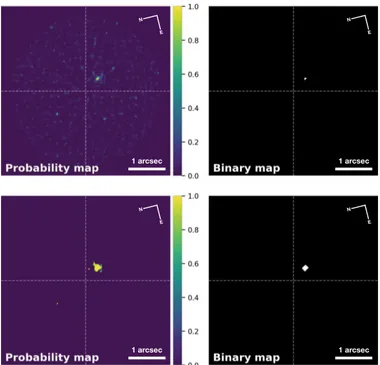
Fig. 4.SODIRF and SODINN outputs for the VLT/NACO β Pic dataset.

Top panelsshow SODIRF’s probability (left) and binary detection maps (right). Bottom panels correspond to SODINN’s output. Both binary detection maps are obtained with a 99% probability threshold. randomly using a Xavier uniform initializer and are learned by back-propagation with a binary cross-entropy cost function:

L= −X

n

(ynln( ˆyn)+ (1 − yn) ln(1 − ˆyn)), (5)

where yn is the true label of the nth MLAR sample and

ˆyn= p(c+| MLAR sample) is the probability that the nth MLAR

sample belongs to the positive class. The architecture of the neural network is not dataset dependent.

The labeled data is divided into train, test (ten percent of the initial labeled samples), and validation sets. The optimization of deep networks, with a large number of parameters, is accom-plished with mini-batch stochastic gradient descent. It works by drawing a random batch from the training set, performing a for-ward pass (running it through the network) to obtain predictions ˆy, computing the loss score on this batch, and the gradient of the loss with regard to the parameters of the network (which is called a backward pass). The parameters or weights are then changed in the direction opposite to the gradient (Chollet 2017). The aim of this process is to lower the loss on the batch by a small step, also called learning rate. The whole process of learning the weights (that minimize the loss) is made possible by the fact that neural networks are chains of differentiable tensor operations. Therefore it is possible to use the backpropagation method, by applying the chain rule of derivation to find the gradient func-tion mapping the current parameters and current batch of data to a gradient value.

We adopt the Adam optimization strategy (Kingma & Ba 2014), which extends classical stochastic gradient descent and computes individual adaptive learning rates for different parame-ters from estimates of first and second moments of the gradients. We use a step size of 0.003 and mini-batches of 64 training samples. We include an early stopping condition monitoring the validation loss. Usually, our model is trained with 15 epochs (passes of the stochastic gradient descent optimizer through the

whole train set) reaching 99.9% validation accuracy. SODINN’s neural network classifier is implemented using the highly mod-ular and minimalist Keras library (Chollet et al. 2015) using its Tensorflow (Abadi et al. 2015) backend. The model is trained on a NVIDIA DGX-1 system using one of its eight P100 cards in about one hour. Training such a network is possible on any com-puter with a dedicated last-generation GPU, such as a NVIDIA TitanX. Almost the same runtime is achieved when training the model on a much cheaper GTX 1080 Ti card installed on a conventional server.

5. Prediction stage

Once the models are trained, they are applied to the input data cube. First, we perform the same transformations (same CEVR intervals) to the input ADI sequence to obtain MLAR patches centered on each one of the pixels of the frame. The discrim-inative model then classifies these MLAR patches, assigning a probability of membership to the positive class, p( ˆy = c+ | MLAR sample). For SODINN, the prediction stage is just a forward pass of a given test sample through the trained deep neural network to produce an output probability. In our super-vised framework, grabbing MLAR patches for each pixel of the frame enables the estimation of a class probability in a detec-tion map. This map is then thresholded at a desired level of c+ class probability. The probability and binary maps are the out-puts of both SODIRF and SODINN, as exemplified in Fig.4for the VLT/NACO dataset. We can see how the binary maps clearly reveal the presence of β Pic b, without false positives (FPs), for this probability threshold.

For comparison, in a differential imaging PCA-based approach, one would tune the number of PCs that works best for a companion at a given radial distance and obtain a residual flux image. This trial and error process leads to a single realiza-tion (using one k value) of the residuals, which is then visually inspected to identify companions or is turned into a S/N map. In the case of our supervised detection method, the predicted proba-bility (or detection criterion) is evaluated independently for each pixel on the frame and does not suffer from the small-sample-statistics issue or, for that matter, human-perception biases. This is a huge improvement compared to differential imaging where the S/N metric requires taking into account the annulus-wise noise at the separation of a given test resolution element.

In order to test the validity of our training procedure, we injected faint fake companions in the ADI sequence used to generate the labeled dataset, without masking the injected com-panions, to simulate the situation when we face a new dataset with real unknown exoplanets. Afterwards, we checked whether the trained models were able to detect these pre-existing com-panions. In this test, the injected companions could be recov-ered with a high success rate, which demonstrates that our approach prevents overfitting at the labeled dataset generation stage. Therefore, we conclude that our framework can be safely applied to new ADI datasets and the performance assessment shown in Sect.6is fair. We would like to emphasize that hav-ing access to multiple datasets taken with the same instrument (survey data), would enable training a more general model and would depend less strongly on the proposed data augmentation procedure.

6. Performance assessment

Testing on known companions is a first sanity check for any exoplanet-detection algorithm. The next step is to proceed with

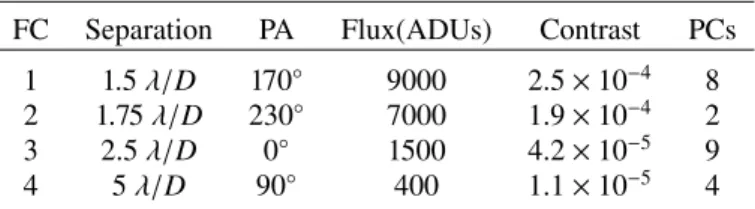
Table 1. Parameters for the fake companions (FC) in Fig.5.

FC Separation PA Flux(ADUs) Contrast PCs

1 1.5 λ/D 170◦ _{9000 2.5 × 10}−4 ₈

2 1.75 λ/D 230◦ 7000 1.9 × 10−4 2

3 2.5 λ/D 0◦ _{1500 4.2 × 10}−5 ₉

4 5 λ/D 90◦ 400 1.1 × 10−5 4

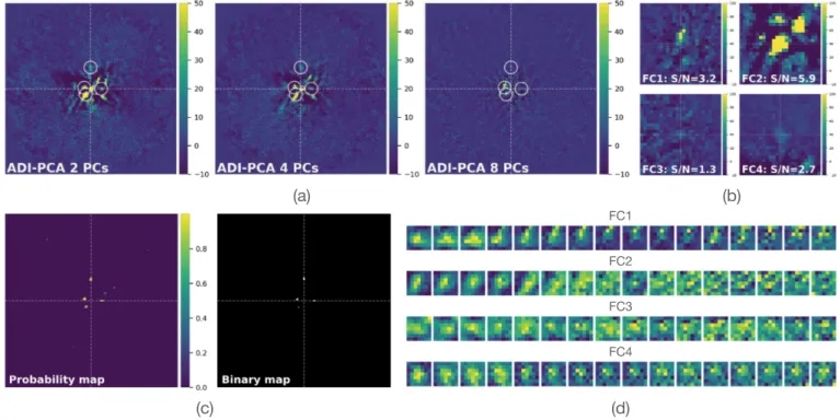
testing the performance (detection capacity) of our trained mod-els by injecting fake companions. In this Section, we focus on SODINN. Using the V471 Tau VLT/SPHERE dataset, a chal-lenging ADI sequence with few frames and mild rotation, we inject four companions (using the input off-axis PSF), at angular separations ranging from one to five λ/D, as indicated in Table1

and illustrated in panel a in Fig5(which shows three realizations of an ADI-PCA residual frame with two, four, and eight PCs subtracted). The first, third, and fourth companions are pretty much at the level of the speckle noise at their corresponding sep-arations. The shapes of their PSFs are hard to distinguish from surrounding noise and the S/N values are small. The quoted S/N in panel b in Fig.5is the best mean S/N, in a 1 × FWHM aperture centered at the injection positions, obtained after optimizing the number of PCs (shown in Table1). Only the second companion has a S/N over five, which is due to the fact that it was purposely injected on top of a bright speckle. The visual inspection would not be definitive for such a companion. As shown in panel c in Fig.5, SODINN outperforms the full-frame ADI-PCA approach by recovering the four companions at a high (99%) probability without any FPs.

Tests with known and injected companions are the first attempts to measure the performance of our supervised detection method. Unfortunately, it is not possible to judge the perfor-mance of a detection algorithm based on a few realizations of such tests. Following Gomez Gonzalez et al.(2016), we use a robust signal detection theory tool for assessing the performance of our exoplanet detection algorithms: the receiver operating characteristic (ROC) curve. This curve is a graphical plot used for assessing the performance of classifiers (see AppendixAfor a more detailed discussion). In general, ROC curves allow us to study the performance of a binary classifier system in a true positive rate (TPR = p(ˆy = c+ | y = c+)) - false positive rate (FPR= 1 − p(ˆy = c− _{|y = c}−_{)) space, as a detection}

thresh-old τ varies. In other words, they can assess the TPR (also called sensitivity) and the FPR at the same time. In Fig. 6, we illustrate the task of a binary classifier in a signal-detection context and the effect of choosing a detection threshold. By varying this threshold, we can adjust the FPR that we are will-ing to accept for a specific sensitivity. A ROC curve shows how good our classification algorithm is for separating the two classes, an ability inherent to the classifier. HCI as a signal-detection problem seeks to maximize the sensitivity to com-panions and minimize the number of false detections (FPR) simultaneously.

In this study, we choose to build our ROC curves in a TPR (percentage of detected fake companions) versus mean per-frame FPs, instead of a TPR versus FPR space. The total number of FPs is counted on the whole detection map, and is averaged for each τ. This reflects better the goal of a planet hunter and facilitates interpretation of the performance simulations. The ROC curves are built separately for different annuli with a tuned uniform flux distribution for the injection of fake companions. Having ROC curves for different separations from the star better illustrates the

Fig. 5.Injection of four synthetic companions (parameters detailed in Table1) in the V471 Tau VLT/SPHERE ADI sequence. The locations of the injections are shown with white circles on the ADI-PCA residual images. Panel a: three ADI-PCA final frames with two, four, and eight PCs subtracted. Panel b: cropped frames centered on the injected companions after optimizing the number of PCs (as shown in Table1) to maximize the S/N of each companion. SODINN’s probability and binary maps clearly reveal the four planets (without false positives at 99% probability) as seen in panel c. Panel d: MLAR patches, used at the prediction stage, centered on each one of the injected companions.

Fig. 6.Behavior of a binary classifier in a signal detection theory

con-text. By varying the detection threshold we can study the classifier’s performance.

algorithm performance at different noise regimes. When inter-preting the results, it is important to compare the ROC curves for different algorithms to one another, for a given annulus, con-sidering that the TPR depends on the brightness of the injected companions, while the mean per-frame FPs does not (see panels b and c in Fig.A.1). It is also important to examine the shape of the curves. For instance, it is preferable to have a steeper curve, which means that such an algorithm does better at minimizing the number of FPs while it increases its sensitivity.

We compare SODINN and SODIRF to classical ADI median subtraction, full-frame ADI-PCA and LLSG on both the VLT/NACO β Pic dataset and the VLT/SPHERE V471 Tau dataset. As mentioned earlier, differential imaging approaches (unsupervised learning), that is, ADI median subtraction, ADI-PCA, and LLSG, do not generate a prediction (probability) but rather a residual image to look at. We obtain detection maps for

these approaches by building S/N maps and thresholding them at several values of τ. For each injection of a fake companion, a new data cube is built and processed with each of the five algorithms. In the case of the VLT/SPHERE V471 Tau dataset, the labeled datasets used for training SODIRF/SODINN are pro-duced using both H2 and H3 SPHERE/IRDIS image sequences, while the prediction step is performed on the H3 band sequence only. The discriminative models are trained once for the ROC-curve analysis. The number of PCs for ADI-PCA and the rank parameter for LLSG are set to two PCs (0.7 CEVR) for the V471 Tau sequence and to nine PCs (0.9 CEVR) for the β Pic one. They are optimized in order to have the best possible ROC curves for ADI-PCA at the considered separations. No other hyperparam-eters were tuned. Signal-to-noise ratio maps were built for the resulting residual frames and thresholded at different values of τ: 0.5, 1, 1.5, 2, 2.5, 3, 3.5, 4, 4.5, 5. For SODINN and SODIRF, we thresholded the probability map at several levels: 0.1, 0.2, 0.3, 0.4, 0.5, 0.59, 0.69, 0.79, 0.89, 0.99. FigureA.2illustrates one single realization of a companion injection, the generation of detection maps, and the thresholding operation for three values of τ. When training SODIRF and SODINN, MLAR samples of 16 slices (in the interval 0.5–0.95 CEVR) are used for the V471 Tau dataset, and 20 slices (in the interval 0.46–0.98 CEVR) for the β Pic sequence.

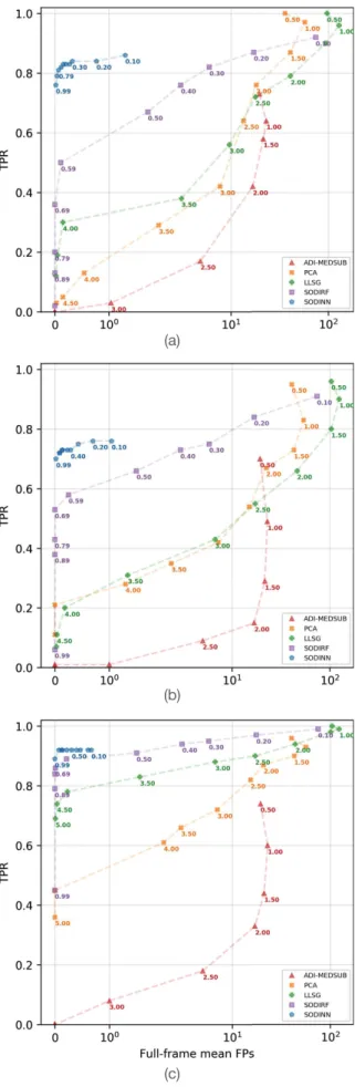
The ROC curves, built for three different annuli, are shown in Figs.7 and8. Brightnesses, contrasts and distances, for all the injected companions (100 for each annulus), are shown in Table2. Reading the ROC curves presented here is straightfor-ward: panel a in Fig.7(annulus from one to two λ/D) shows that a blob, that is, at least two active pixels inside a 3 × 3-pixel box centered at the position of the fake companion injection, sticks out above the detection threshold in 16%, 28%, ∼42%, ∼44% and ∼68% of the cases for ADI median subtraction, ADI-PCA,

Fig. 7.ROC curves for the VLT/SPHERE V471 Tau dataset, compar-ing ADI median subtraction, ADI-PCA, LLSG, SODIRF and SODINN. The panels show ROC curves built for different separations: a) 1–2 λ/D, b) 2–3 λ/D and c) 4–5 λ/D. The contrasts are shown in Table2.

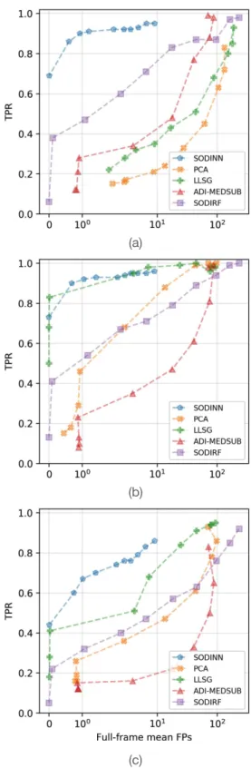
Fig. 8.Same as Fig.7for the VLT/NACO β Pic dataset. The contrasts

are shown in Table2. The labels denote the detection thresholds: S/N for ADI median subtraction, ADI-PCA, and LLSG, and probabilities for SODIRF and SODINN.

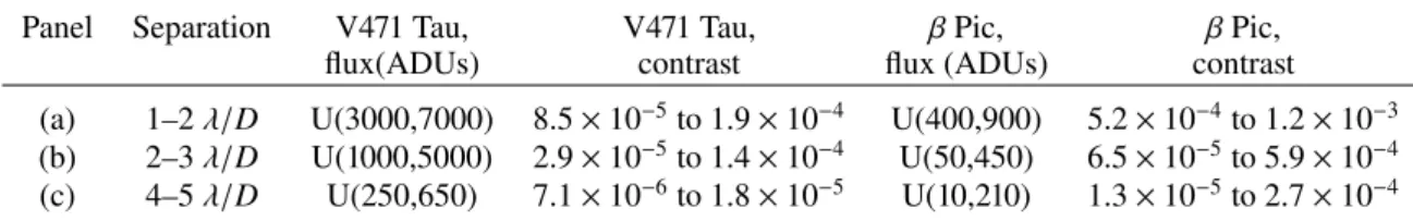
Table 2. Parameters used for the ROC curves in Figs.7and8.

Panel Separation V471 Tau, V471 Tau, β Pic, β Pic,

flux(ADUs) contrast flux (ADUs) contrast

(a) 1–2 λ/D U(3000,7000) 8.5 × 10−5to 1.9 × 10−4 U(400,900) 5.2 × 10−4to 1.2 × 10−3 (b) 2–3 λ/D U(1000,5000) 2.9 × 10−5_{to 1.4 × 10}−4 _{U(50,450) 6.5 × 10}−5_{to 5.9 × 10}−4

(c) 4–5 λ/D U(250,650) 7.1 × 10−6to 1.8 × 10−5 U(10,210) 1.3 × 10−5to 2.7 × 10−4

LLSG, SODIRF, and SODINN, respectively, and for an average of ∼0.8 FPs in the full-frame detection map. The ROC curves for different separations and two very different datasets (from dif-ferent HCI instruments) consistently show SODINN’s improved performance with respect to other approaches. SODIRF’s sen-sitivity improves with the separation and starts to match the performance of SODINN. In Appendix A, we provide more details about the construction of the ROC curves for the assess-ment of exoplanet-detection algorithms. For instance, we show that hyperparameter tuning is important and the curves for ADI-PCA and LLSG could be slightly improved by searching the optimal number of PCs at each separation.

7. Conclusions

This study illustrates the potential of machine learning in HCI for the task of exoplanet detection. We present a novel paradigm for detecting point-like companions in ADI sequences by refor-mulating HCI post-processing as a supervised learning problem, building on well-established machine learning techniques. Instead of relying on unsupervised learning techniques, as most of the state-of-the-art ADI post-processing algorithms do, we generate labeled datasets (MLAR samples) and train discrim-inative models that classify each pixel of the image, assigning a probability of containing planetary signal. We present two approaches that differ in the type of discriminative model used: SODIRF and SODINN. The former employs a random-forest classifier, while the latter features a more advanced deep neural network model, which better exploits the structure of the labeled MLAR samples.

In order to assess the detection capabilities of our approaches, we perform a ROC analysis comparing both SODINN and SODIRF to ADI median subtraction, ADI-PCA, and LLSG techniques. The performances of both algorithms are beyond what ADI-PCA and ADI median subtraction can offer. SODIRF can be considered as a computationally cheap alterna-tive to the deep neural network approach of SODINN, whose performance lies in a separate zone of the ROC space. From one to two λ/D, SODINN improves the TPR by a factor of ∼2 and ∼10, for two different datasets, with respect to ADI-PCA and LLSG when working at the same false-positive level. Moreover, the improvement in discriminating planet signal from speckles holds in the case of a challenging ADI sequence, with mild rotation and few frames, from a last-generation HCI instrument – VLT/SPHERE (see Appendix Afor a more detailed discus-sion of the ROC-curves performance assessment). The fact that these models are versatile and can be fine-tuned to each specific ADI sequence opens great possibilities of re-processing existing databases, from first- and second-generation HCI instruments, to maximize their scientific return.

Although in this study we only addressed single ADI datasets, our framework’s true potential is in the context of sur-veys, where the data from different observations could be used

to generate a larger and more diverse labeled dataset. This would enable more efficient and more general deep neural network models for SODINN. The exploitation of SODINN for surveys will be the focus of a future study. Other interesting avenues of future research are the inclusion of the companion brightness into the model, the extension to other HCI observing techniques (beyond ADI), and the use of generative neural networks for complementing the data augmentation process.

The simultaneous increase in sensitivity, which translates to deeper detection limits (the ability to detect companions at higher contrasts), and reduction of the per-image FPs, clearly indicate that our supervised approach SODINN is a very pow-erful HCI exoplanet detection technique. Considering that ADI remains the most common HCI observing strategy, and given the large reservoirs of archival data, SODINN could potentially improve the demographics of directly imaged exoplanets at all separations, including those in the inner vicinity (1–2 λ/D) of their parent stars where ADI signal self-subtraction and speckle noise are the strongest.

Acknowledgements.The authors would like to thank the python open-source scientific community and the developers of the Keras deep learning library. The authors acknowledge fruitful discussions and ideas from the participants in the Exoplanet Imaging and Characterization workshop organized by the W.M. Keck Institute for Space Studies. The research leading to these results has received funding from the European Research Council Under the European Union’s Seventh Framework Program (ERC Grant Agreement n. 337569) and from the French Community of Belgium through an ARC grant for Concerted Research Action.

References

Abadi, M., Agarwal, A., Barham, P., et al. 2015, ArXiv e-prints: [arXiv:1603.04467],software available from tensorflow. org

Absil, O., Milli, J., Mawet, D., et al. 2013,A&A, 559, L12 Amara, A., & Quanz, S. P. 2012,MNRAS, 427, 948

Ball, N. M., & Brunner, R. J. 2010,Int. J. Mod. Phys. D, 19, 1049

Barrett, H. H., Myers, K. J., Devaney, N., Dainty, J. C., & Caucci, L. 2006, in Advances in Adaptive Optics II.,eds. B. L. Ellerbroek, & D. Bonaccini Calia, Proc. SPIE, 6272, 1W

Bertin, E., & Arnouts, S. 1996,A&AS, 117, 393

Beuzit, J.-L., Feldt, M., Dohlen, K., et al. 2008, inGround-based and Air-borne Instrumentation for Astronomy II, eds. I. S. McLean, & M. M. Casali, Proc. SPIE, 7014, 701418

Boureau, Y.-L., Ponce, J., & LeCun, Y. 2010, inICML, eds. J. Fürnkranz & T. Joachims (Madison, WI: Omnipress),111

Bowler, B. P. 2016,PASP, 128, 102001

Braham, M., & Van Droogenbroeck, M. 2016,Int. Conf. on Systems, Signals and Image Processing, held in Bratislava, Slovakia

Breiman, L. 2001,Machine Learning, 45, 5

Cantalloube, F., Mouillet, D., Mugnier, L. M., et al. 2015,A&A, 582, A89 Chollet, F. 2017,Deep Learning with Python(Shelter Island, NY: Manning

Publications)

Chollet, F., et al. 2015,Keras,https://github.com/fchollet/keras Dieleman, S., Willett, K. W., & Dambre, J. 2015,MNRAS, 450, 1441

Dohlen, K., Langlois, M., Saisse, M., et al. 2008, inGround-based and Air-borne Instrumentation for Astronomy II, eds. I. S. McLean, & M. M. Casali, Proc. SPIE, 7014, 70143L

Fergus, R., Hogg, D. W., Oppenheimer, R., Brenner, D., & Pueyo, L. 2014,ApJ, 794, 161

Flamary, R. 2016, ArXiv e-prints [arXiv:1612.04526]

Frontera-Pons, J., Sureau, F., Bobin, J., & Le Floc’h, E. 2017,A&A 603, A60 Gomez Gonzalez, C. A., Absil, O., Absil, P.-A., et al. 2016,A&A, 589, A54 Gomez Gonzalez, C. A., Wertz, O., Absil, O., et al. 2017,AJ, 154, 7

Goodfellow, I., Bengio, Y., & Courville, A. 2016,Deep Learning(Cambridge, MA: MIT Press),http://www.deeplearningbook.org

Graham, J. R., Macintosh, B., Doyon, R., et al. 2007, ArXiv e-prints [arXiv:0704.1454]

Halko, N., Martinsson, P.-G., & Tropp, J. A. 2011,SIAM Review, 53, 217 Hardy, A., Schreiber, M. R., Parsons, S. G., et al. 2015,ApJ, 800, L24 Hinton, G. E., Srivastava, N., Krizhevsky, A., Sutskever, I., & Salakhutdinov, R.

2012, ArXiv e-prints [arXiv:1207.0580]

Hochreiter, S., & Schmidhuber, J. 1997,Neural Comput., 9, 1735 Hoyle, B. 2016,Astron. Comput., 16, 34

Kenworthy, M. A., Codona, J. L., Hinz, P. M., et al. 2007,ApJ, 660, 762 Kim, E. J., & Brunner, R. J., 2017,MNRAS, 464, 4463

Kingma, D. P., & Ba, J. 2014, ArXiv e-prints [arXiv:1412.6980]

Krizhevsky, A., Sutskever, I., & Hinton, G. E. 2012, in Advances in Neural Information Processing Systems, 1097

Lafrenière, D., Marois, C., Doyon, R., Nadeau, D., & Artigau, É. 2007,ApJ, 660, 770

Lagrange, A.-M., Bonnefoy, M., Chauvin, G., et al. 2010,Science, 329, 57 Lawson, P. R., Poyneer, L., Barrett, H., et al. 2012, inAdaptive Optics Systems

III,Proc. SPIE, 8447, 844722

LeCun, Y., Jackel, L. D., Boser, B., et al. 1989,IEEE Commun. Mag., 27, 41 Louppe, G. 2014, Ph.D. Thesis, University of Li, Belgium,

https://github.com/glouppe/phd-thesis[arXiv:1407.7502] Marois, C., Lafrenière, D., Doyon, R., Macintosh, B., & Nadeau, D. 2006,ApJ,

641, 556

Marois, C., Macintosh, B., Barman, T., et al. 2008,Science, 322, 1348 Marois, C., Zuckerman, B., Konopacky, Q. M., Macintosh, B., & Barman, T.

2010,Nature, 468, 1080

Masias, M., Freixenet, J., Lladó, X., & Peracaula, M. 2012,MNRAS, 422, 1674 Mawet, D., Riaud, P., Absil, O., & Surdej, J. 2005,ApJ, 633, 1191

Mawet, D., Milli, J., Wahhaj, Z., et al. 2014,ApJ, 792, 97

Milli, J., Mawet, D., Mouillet, D., Kasper, M., & Girard, J. H. 2016, inAstronomy at High Angular Resolution, (Springer) 439, 17

Mugnier, L. M., Cornia, A., Sauvage, J.-F., et al. 2009, J. Opt. Soc. Am. A, 26, 1326

Nair, V., & Hinton, G. E. 2010, inICML, eds. J. Fürnkranz & T. Joachims (Madison, WI: Omnipress),807

Odewahn, S. C., Stockwell, E. B., Pennington, R. L., Humphreys, R. M., & Zumach, W. A. 1992,AJ, 103, 318

Rouan, D., Riaud, P., Boccaletti, A., Clénet, Y., & Labeyrie, A. 2000,PASP, 112, 1479

Ruffio, J.-B., Macintosh, B., Wang, J. J., et al. 2017,ApJ, 842, 14

Rumelhart, D. E., Hinton, G. E., & Williams, R. J. 1986, inParallel Distributed Processing, eds. D. E. Rumelhart & J. L. Mcclelland, (Cambridge, MA: MIT Press),1, 318

Schawinski, K., Zhang, C., Zhang, H., Fowler, L., & Santhanam, G. K. 2017, MNRAS, 467, L110

Shi, X., Chen, Z., Wang, H., et al. 2015, inNIPS(Cambridge, MA: MIT Press), 802

Soummer, R. 2005,ApJ, 618, L161

Soummer, R., Pueyo, L., & Larkin, J. 2012,ApJ, 755, L28 Sparks, W. B. & Ford, H. C. 2002,ApJ, 578, 543 Spergel, D., & Kasdin, J. 2001, inBAAS, 33, 1431

Srivastava, N., Hinton, G. E., Krizhevsky, A., Sutskever, I., & Salakhutdinov, R. 2014, J. Mach. Learn. Res., 15, 1929

Tagliaferri, R., Longo, G., Milano, L., et al. 2003,Neural Networks, 16, 297 Tran, D., Bourdev, L. D., Fergus, R., Torresani, L., & Paluri, M. 2015, inICCV

(IEEE Computer Society), 4489

Xie, D., Zhang, L., & Bai, L. 2017,Appl. Comp. Int. Soft Comput., 2017, 13, 1320780

Appendix A: Construction of ROC curves

ROC curves are commonly used statistical tools for assessing the performance of binary classifiers. The planet detection task, where we are interested in evaluating the algorithm’s sensitiv-ity or abilsensitiv-ity to detect planets of varying contrast (brightness with respect to the star), can be seen as a binary classification. Therefore, ROC curves can be used for algorithm-performance assessment in HCI (Barrett et al. 2006;Lawson et al. 2012). A ROC curve shows a classifier TPR-FPR trade-off as a function of a detection threshold τ.

It is important to understand that the relative ROC per-formance of two different algorithms changes due to several factors: the dataset used (which has a set of characteristics such as the total rotation range, integration time, total number of frames, weather condition, wavefront control system perfor-mance and coronagraphic solution), hyper-parameter tuning of each algorithm (as shown in Fig. A.1), noise regime or sepa-ration from the star, and contrast of the injected companions (as shown in Fig. A.1). There is no shortcut to avoiding the dependence on these factors, unless the metric makes strong assumptions about the data and noise distributions (which are rarely confirmed in practice). A data-driven approach to the calculation of ROC curves, using standardized datasets, is the most fair and reliable method for assessing the performance of HCI algorithms. The ROC curves shown in this work, for the case of a single ADI dataset, are generated in the following way:

1. An on-sky dataset is chosen. Any high S/N or known com-panion is removed, for example, using the negative fake companion technique (Lagrange et al. 2010; Marois et al. 2006;Gomez Gonzalez et al. 2017).

2. A separation from the star (1 × FWHM annulus) and a planet-to-star contrast interval (the brightness of the injected companions) are selected. A list of τ thresholds is also defined.

3. A large enough number of data cubes are built with a single injected companion at the selected separation and within the chosen contrast interval.

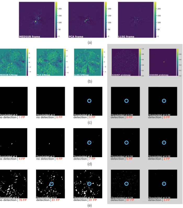
4. The data cubes are processed with each algorithm involved in the performance assessment/comparison. Panel a in Fig. A.2 shows the resulting residual flux frames for the model PSF subtraction approaches. Panel b shows the result-ing probability maps of SODIRF and SODINN. S/N maps are produced from the residual flux frames (see panel b in Fig.A.2).

5. Binary maps are obtained by thresholding the S/N and prob-ability maps for different values in τ (see panels c–e in Fig. A.2). For each detection map and for each τ, a true positive is counted if a blob is recovered at the injection loca-tion. False positives are other significant blobs at any other location in the detection map.

6. For each τ, the true positives and the number of FPs are averaged.

When choosing a dataset, we must subtract known and high-S/N existing companions, based on visual vetting performed on a model PSF-subtracted residual image. As shown in this study, the PSF subtraction methods combined with visual vetting and S/N metrics are far from obtaining 100% probability of finding companions and therefore obtaining an empty dataset. Never-theless, the only choice is to assume the sequence is empty, or free of astrophysical exoplanetary signal, and flag any potential companion as a FP in the following steps of the ROC curve gen-eration procedure. In the last step, averaging the number of FPs

Fig. A.1. Exemplification of the pitfalls of comparative studies using

ROC curves, and how easy it is to obtain incorrect relative performances and present inaccurate conclusions. These ROC curves are built for the same dataset and separation from the star. Panels a and b: ROC curves when changing the algorithms hyper-parameters: the number of PCs for ADI-PCA and the rank of LLSG. In panel a a more aggressive value is used with respect to panel b. The performance of ADI-PCA and LLSG is worst when too aggressive hyper-parameters are used. We notice how their curves move upward in panel b with respect to ADI median subtraction, SODIRF, and SODINN curves. Panel c is gener-ated by injecting fainter companions with respect to panel b. A higher planet-to-star contrast interval is a more sensible choice for highlighting the relative sensitivity of the studied algorithms.

Fig. A.2.Case of a single injection for building a ROC-curve comparative analysis. Panel a: groups the final residual frames for the model PSF subtraction approaches (ADI median subtraction, ADI-PCA and LLSG). Detection maps are shown in panel b: S/N maps from the residual flux frames of panel a and probability maps of SODIRF and SODINN. Panels c–e: binary maps obtained from the thresholded S/N and probability maps of panel b. The detected fake companion is shown with a blue circle on the binary maps. The detection state and the number of FPs are also shown next to each binary map. We highlight that the number of FPs grows when τ is decreased and also that SODINN controls the number of FPs. A large number of these injections (with varying flux and position) need to be performed in order to build the ROC curves.

(instead of assuming a static noise realization per τ) addresses small fluctuations in this value, caused by the interaction of an

injected companion with the FPs at the same separation (which biases the S/N).