Belgian National Committee for Theoretical and Applied Mechanics

ECCOMAS N

EWSLETTER

J

ANUARY

2017

E

UROPEAN

C

OMMUNITY ON

C

OMPUTATIONAL

M

ETHODS IN

A

PPLIED

S

CIENCES

C

ONTENTS

M

ESSAGE

O

F

T

HE

P

RESIDENT...3

E

KKEHARD

R

AMM

H

OW

A

PPLIED

S

CIENCES

C

AN

A

CCELERATE

T

HE

E

NERGY

R

EVOLUTION -

A

P

LEADING

F

OR

E

NERGY

A

WARENESS

I

N

S

CIENTIFIC

C

OMPUTING ………...7

M

ARKUS

G

EVELER,

S

TEFAN

T

UREK

T

HE

V

IRTUAL

E

LEMENT

M

ETHOD:

A

N

EW

P

ARADIGM

F

OR

T

HE

A

PPROXIMATION

O

F

P

ARTIAL

D

IFFERENTIAL

E

QUATION

P

ROBLEMS ……….…….15

C

ARLO

L

OVADINA

A

NDERSON

L

OCALIZATION

I

N

A B

ALLASTED

R

AILWAY

T

RACK ………...20

R

.

C

OTTEREAU,

L. D

E

A

BREU

C

ORRÊA,

E. B

ONGINI,

S

.

C

OSTA

D

’

A

GUIAR,

B

.

F

AURE,

C

.

V

OIVRET

G

ENERAL-

P

URPOSE

C

ONTRAST-

P

RESERVING

V

ISUALIZATION

O

F

H

IGH

D

YNAMIC

R

ANGE

D

ATA

I

N

U

NCERTAINTY

Q

UANTIFICATION ……….………...25

J

UHA

J

ERONEN

VII ECCOMAS CONGRESS

……….………...………...30

W

HO

R

EPRESENTS

C

OMPUTATIONAL

M

ECHANICS

R

ESEARCH

I

N

T

HE

UK

?

U.K.A.C.M.

…….……….…...34

C

HARLES

A

UGARDE

B

ELGIAN

N

ATIONAL

C

OMMITTEE

F

OR

T

HEORETICAL

A

ND

A

PPLIED

M

ECHANICS ………...………….36

J

EAN

P

HILIPPE

P

ONTHOT

6

TH

E

UROPEAN

C

ONFERENCE

O

N

C

OMPUTATIONAL

M

ECHANICS -

7

TH

E

UROPEAN

C

ONFERENCE

O

N

C

OMPUTATIONAL

F

LUID

D

YNAMICS ...37

E

CCOMAS

T

HEMATIC

C

ONFERENCES 2017...38

E

CCOMAS

Y

OUNG

I

NVESTIGATORS

C

ORNER …..………...40

4

TH

E

CCOMAS

Y

OUNG

I

NVESTIGATORS

C

ONFERENCE 2017 -

PHD O

LYMPIAD 2017 …...42

ECCOMAS NEWSLETTER — JANUARY 2017 ALL RIGHTS RESERVED BY AUTHORS.

EDITORS

EKKEHARD RAMM

UNIVERSITÄT STUTTGART

PRESIDENT OF ECCOMAS

MANOLIS PAPADRAKAKIS

NATIONAL TECHNICAL UNIVERSITY OF ATHENS

PAST PRESIDENT OF ECCOMAS

BERT SLUYS

DELFT UNIVERSITY OF TECHNOLOGY

MEMBER OF THE MANAGING BOARD OF ECCOMAS

GUEST EDITOR

JOSEF EBERHARDSTEINER

VIENNA UNIVERSITYOF TECHNOLOGY

SECRETARY OF ECCOMAS

TECHNICAL EDITOR

PANAGIOTA KOUNIAKI

M

ESSAGE OF THE

P

RESIDENT

N

EWSLETTER

F

OR

E

CCOMAS

C

ONFERENCES

I

N

2017

The main purpose of the current ECCOMAS Newsletter is that it will be distributed in particular to all participants of ECCOMAS Conferences in 2017. These are the 35 Thematic Conferences (TC) (http://eccomas.cimne.com/

vpage/1/14/2017) and the ECCOMAS Young Investigators Conference YIC 2017, see below. The TCs cover the entire thematic spectrum of ECCOMAS from Computational Solid & Structural Mechanics (CSM), Fluid Dynamics (CFD), and Applied Mathematics (CAM) to Scientific Computing (SC); traditionally an emphasis lies on topics within CSM. Most of the meetings are part of a series of conferences which took place in several previous years before. One conference is in particular worth mentioning, namely the International Conference on Computational Plasticity (COMPLAS) which started 30 years ago, some time before ECCOMAS was founded. As some other TCs it has a strong intercontinental orientation

indicated by the label “IACM Special Interest Conference”.

Originally ECCOMAS Thematic Conferences were supposed to be small highly specialized meetings with up to 100 attendees. However it turned out that the format was also best suited for medium size

conferences of up to 450 participants still focused on a main topic. In 2015 over 3700 people attended the 25 Thematic Conferences. In 2017 we face the 7th edition with a substantial increase in number of conferences. It can be stated that the system of ECCOMAS Thematic Conferences taking place in odd years is really a success story.

F

URTHER

F

UTURE

C

ONFERENCES

For 2017 I again would like to refer to the ECCOMAS Young Investigators Conference YIC 2017 organized by the Polytechnic University of Milan 13-15 September 2017 (https:// www.eko.polimi.it/index.php/ YIC2017/conf). It is chaired by Massimiliano Cremonesi, Assistant Professor at POLIMI, and is the 4th edition of the series of YICs after those in Aveiro (Portugal), Bordeaux (France) and Aachen (Germany). YIC Conferences are exclusively organized in odd years and run by Young Investigators, or – as we used to say - “for young scientists from

young scientists”, i.e. the target groups are PhD students in all stages of their PhD programs, postdocs and young researchers from academia and industry under the age of 35.

YIC 2017 comes along with the 7th ECCOMAS PhD Olympiad. In this event every Member Association is represented by a number of selected PhDs submitted for consideration for the two ECCOMAS PhD awards (http:// eccomas.cimne.com/vpage/1/18/ RulesConditions).

As known ECCOMAS organizes the European Conferences on Computational Mechanics (Solids, Structures and Coupled Problems) ECCM and on Computational Fluid Mechanics ECFD in even years, alternating with the ECCOMAS Congress; the last Congress took place in Crete 2016 with over 2200 participants. ECCOMAS decided again merging the two Conferences in 2018 under the condition that the two individual parts have equal rights and keep their own identity. This joint ECCM – ECFD 2018 Conference takes place in Glasgow (UK) 11-15 June 2018 (http:// www.eccmecfd2018.org/frontal/ default.asp). It is hosted by the University of Glasgow and the University of Edinburgh and organized in partnership with the UK

E

UROPEAN

C

OMMUNITY ON

C

OMPUTATIONAL

M

ETHODS IN

A

PPLIED

S

CIENCES

Association for Computational Mechanics in Engineering (UKACM). For ECCOMAS it is a very special conference because the Association celebrates its 25th anniversary during the meeting.

The calls for the Thematic Conferences as well as the YIC conference in 2019 have already been started end of last year. The final decisions on this issue are scheduled for the board meetings of ECCOMAS in May 2017.

Joining big conferences makes a lot of sense when clusters of big conferences in close thematic neighborhood take place in the same period of the respective year. This is true in 2018 and will be also the case in 2020. The International Association for Computational Mechanics (IACM) organizes their World Conference WCCM again in Europe. It was obvious that both organizations IACM and ECCOMAS decided merging again their main conference events in 2020, as it was successfully done previously. After a

joint call for tender leading to excellent proposals, and a secret selection procedure by their main boards both associations decided to choose Paris as the venue for the combined ECCOMAS Congress 2020 and the 14th World Conference on Computational Mechanics on 19-24 July, 2020.

E

CCOMAS

A

DVANCED

C

OURSES

, S

CHOOLS

A

ND

W

ORKSHOPS

ECCOMAS’ Bylaws define among others the objective to stimulate and promote education in its field of operation. Following this objective the Managing Board decided in its meeting in Crete 2016 to launch a program for the organization of

ECCOMAS Advanced Courses, Schools and Workshops, for simplicity denoted as ECCOMAS Advanced Courses (EAC). The project could be denoted a twin program to the successful series of Thematic Conferences.

Three different types of Advanced Courses can be distinguished:

1. Stand-alone courses not related to other ECCOMAS events or other scientific institutions, in arbitrary times and locations in Europe,

2. Courses in cooperation with other scientific institutions, as for example the CISM-ECCOMAS International Summer Schools, 3. Courses taking place in the

framework of ECCOMAS events, such as ECCOMAS Congresses, ECCM and ECFD Conferences and ECCOMAS Thematic Conferences, as pre- or post- conference events.

Equivalent to the procedure for the TCs ECCOMAS will support each EAC by disseminating the event via entries in its website, through regular email announcements, on conferences and its newsletter. Further rules and conditions are defined on the website:

http://eccomas.cimne.com/ space/1/19/advanced-schools-and-courses.

I would like to mention two very successful examples for EACs, the CISM-ECCOMAS International

Summer School 2016 on Fluid-Structure Interaction in Udine and the ECCAM Advanced School on Isogeometric Analysis in Crete in connection with the ECCOMAS Congress 2016.

As for the Thematic Conferences also the Advanced Courses should follow the ECCOMAS corporate visual identity; related brochure templates with a dual layout are given on the website. They allow enough flexibility for the individual layout of the respective event. For the homepages of courses see the examples for the TCs in the website.

The ECCOMAS community is encouraged to join this program which could and should be as successful as the TCs.

A

WARDS

After conducting severe selection processes several ECCOMAS Awards could be presented during the ECCOMAS Congress 2016 in Crete. It is important to note that candidates for the ECCOMAS Medals as well as the young scientist awards can be nominated by every individual member of ECCOMAS or from the member associations. The awardees are selected by an award committee by secrete voting.

The highest distinction, the Ritz-Galerkin Medal, was awarded to Franco Brezzi, Professor of Mathematics at the University of

Pavia, Italy, for his outstanding, sustained contributions in computational methods in applied sciences during a substantial portion of his professional life, so to speak as a “life time award”. Two distinguished scientists were honored for their brilliant work in a selected field: Professor Ferdinando Auricchio, U Pavia, for computational solid and structural mechanics by the Leonard Euler Medal, and Wolfgang A. Wall, TU Munich, for computational fluid dynamics by the Ludwig Prandtl Medal. The two awards for young scientists, the Lions Award in Computational Mathematics and the Zienkiewicz Award in Computational Engineering Sciences, were presented to Lourenco Beirão da Veiga, U Milano, and Antonio Javier Gill, U Swansea, respectively.

The best PhD thesis awards for the year 2015 were proposed by ECCOMAS Member Associations and selected by a PhD Awards Committee. The winners were Ursula Rasthofer, TU Munich, and

Federico Negri, EPFL Lausanne.

We from ECCOMAS congratulate all awardees for their excellent research.

R

ESUME

The four years term of the present administration ends in May 2017. An assessment of our work can and should only be done by the membership. We tried to improve the management for the association and consolidate existing building blocks, but also implement new structures. These elements are related to the efficiency of the three boards, General Assembly, Managing Board, and Executive Committee, the reactivation of the four ECCOMAS Technical Committees, and definition and refinement of rules and conditions for the major activities of our Association. I would like to refer to a few selected actions:

safeguarding the financial situation for the future, nomination and selection of awards, set up rules and

Franco Brezzi Ferdinando Auricchio

Wolfgang A. Wall Lourenco Beirão da Veiga

Antonio Javier Gil Ursula Rasthofer Federico Negri

Euler Medal Ritz-Galerkin

Medal Prandtl Medal Lions Award

Zienkiewicz

E

UROPEAN

C

OMMUNITY ON

C

OMPUTATIONAL

M

ETHODS IN

A

PPLIED

S

CIENCES

conditions for all conferences, proposal and selection of plenary and semi-plenary lecturers for the large ECCOMAS Conferences, improving the dissemination of ECCOMAS activities, update the content of the website, establish a new program for ECCOMAS Advanced Courses, Schools and Workshops (see above), renewal of the cooperation with the Centre for Mechanical Sciences (CISM) in Udine, etc. A particular important aspect was the reactivation of the ECCOMAS Young Investigator Committee (EYIC). It turned out that the group started with a new momentum coming up with a lot of novel ideas. I have to confess that this was a special highlight in my term as president.

Of course we also faced the one or the other difficulty in running such a scientific association like ECCOMAS, based on voluntary input and a lot of idealism of the acting members in the administration. We recognized that the information flow between us as the officers and members of boards and committees on the one hand and the individual members of the member associations on the other hand was by far not optimal. Having only national and regional associations as members of ECCOMAS and no direct link to their personal members is a situation which should be reconsidered in the future. Based on a suggestion of the Managing Board the Executive Committee recently started an intensive discussion how this

obstacle and some other difficulties can be overcome. Respective recommendations will be made for the next administration.

T

HANKS

I would like to express my particular thanks to all who substantially supported our work in ECCOMAS. Let me start with Manolis Papadrakakis and his team in Athens for the perfect organization of the wonderful ECCOMAS Congress 2016 in Crete. It was a great success. Thanks also to Bert Sluys for preparing the present Newsletter as a guest editor together with Panagiota Kouniaki in Athens as technical editor in a perfect manner, and to all authors for their contributions.

The support by the officers in the Executive Committee (EC), in particular by both Vice-presidents Ferdinando Auricchio and Pedro Diez and the Treasurer Rémi Abgrall, is highly appreciated. Without the extraordinary assistance by the Secretary Josef Eberhardsteiner my work as President would have not been possible; thank you so much for the exchange of many ideas and initiatives over the entire time.

The commitment of the heads in our Barcelona office, Iztok Potokar and since March 2016 Cristina Forace, was and is of great value for all of us.

I am also grateful for the support by the members of the boards, in particular in the Managing Board (MB); I appreciate the constructive input and the positive working atmosphere. I would like to include the chairmen of the four Technical Committees and of the Young Investigator Committee for their assistance in many aspects of the daily work; it was a definite advantage including them as guest members in the EC and the MB.

Last but not least we all should be thankful for all personal members being engaged in the many activities of ECCOMAS, especially as conference and mini-symposium organizers, lecturers and participants. Their contributions make ECCOMAS a very successful scientific organization with a great promise for the future. For me as President it was a valuable experience. The best wishes go to the new administration!

E

KKEHARD

R

AMM

P

RESIDENT OF

ECCOMAS

RAMM@IBB.UNI-STUTTGART.DE

Ekkehard Ramm Ferdinando Auricchio Pedro Diez Josef Eberhardsteiner Rémi Abgrall Cristina Forace

COMMUNICATED BY CARSTEN CARSTENSEN, CHAIRMAN OF THE ECCOMAS TECHNICAL COMMITTEE "SCIENTIFIC COMPUTING"

H

OW

A

PPLIED

S

CIENCES

C

AN

A

CCELERATE

T

HE

E

NERGY

R

EVOLUTION

-

A P

LEADING

F

OR

E

NERGY

A

WARENESS

I

N

S

CIENTIFIC

C

OMPUTING

1 I

NTRODUCTION

1.1 SCIENTIFIC COMPUTING

CANNOT

CONTINUE TO BE

DONE

THE WAY IT HAS BEEN

There is no denial that the transition from nuclear- and fossil-driven energy supplies to more sustainable options is one of the most challenging tasks of our time. While this transitioning is usually referred

to as ‘the energy revolution’ its basic pillars are not limited to alternative energy production but also are agreed to include better energy grids as well as more energy-efficient consumers. In this sense computing in general and particularly scientific computing as the basic tool for applied sciences contain a great deal of energy consumption since the computers (devices), compute clusters and data

-/compute centers do.

Recently the Semiconductor Industry Association (SIA) released a report where a prediction on the world’s total energy production was made alongside an analogous prediction for the energy consumption of the world’s computers *SIA 2015+. In order to demonstrate the urgency of what shall later be proposed here let us first summarize these findings. For this purpose consider Figure 1. Here the world’s total energy production is extrapolated with a comparatively slow increase leveling out at approximately one Zettajoule in 2015. Speaking on these scales this value is not expected to increase much in this century. On the demand side energy consumption due to usage of computers is expected to increase much faster: Based on current technology (with today’s (digital) computer technology and the way single devices are built and clustered to larger units) the total energy consumed (only by computing) will exceed the world’s energy Figure 1. Prediction of world’s total energy production and overall energy consumption by

E

UROPEAN

C

OMMUNITY ON

C

OMPUTATIONAL

M

ETHODS IN

A

PPLIED

S

CIENCES

production and supply by around 2040. Even based on extrapolating current technology to a hypothetical future technology level (mainly based on improved manufacturing processes leading to smaller transistors) this would lead to only an insignificant delay of this point in time. Consider this as the catastrophe that it is: No additional electrical device would be able to be plugged into the power grid any more. Applications on the other side are continuing to increase their hunger for ever more computational resources. Consider the lowest plot in Figure 1. It represents a theoretical lower bound for the energy consumption per year based on a hypothetical device that needs the minimum amount of energy to flip a bit of information. This limit is called the Landauer Limit. Due to an increasing demand for computational capacities this limit will also be increasing over time since more and more computers will be built. It is more or less increasing with the same rate as today’s or close future’s computer systems’ consumption and such optimal computers would therefore also only postpone the inevitable.

1.2 HARDWARE AND SOFTWARE

IN APPLIED SCIENCES ARE BLIND

ON THE ‘ENERGY EYE’

Today’s compute and data centers mostly rely on massively parallel distributed memory clusters. The compute nodes are also multilevel parallel and heterogeneous. They usually comprise one or more high-end server CPUs based on the x86, Power, or SPARC architectures optionally accelerated by GPUs or other (accelerator) hardware. Large HPC sites of this type have substantial energy requirements so that the associated expenses over the lifetime of the system may

exceed the initial acquisition costs. In addition, the energy supply for supercomputers is not always an integral part of its overall design - consumers (such as the compute cluster, cooling, networking, management hardware) are often developed independently from the key technologies of the energy revolution, e.g. renewable energy sources, battery and power grid techniques. Taking a look at the largest supercomputers today it can be observed that as a consequence of decades of performance-centric hardware development there is a huge gap between pure performance and energy efficiency in these designs: The Top500 list’s best performing HPC system (dissipating power in the 20 Megawatts range making a power supply by local solar farming for instance an impossible-to-achieve aim) is only ranked 84th on the corresponding Green500 list whereas the most energy-efficient system in place only performs 160th in the metric of raw floating point performance *Meuer et al. 2015; Feng et al. 2015+. It is well known *Schӓppi et al. 2009+ *Lawrence Berkeley National Laboratory 2006+ that 40–60% of the energy consumption of an HPC site can be attributed to the compute nodes (processors and memories).

Using and developing scientific

software on the other hand requires

knowledge of the specific target hardware architecture which implies adjustments of numerical methods and their implementation. Otherwise efficiency losses are axiomatic and always imply too much energy spent. Therefore scientific software should not follow a hardware-oblivious design paradigm. In the resulting performance engineering studies for decades energy efficiency has been eclipsed by computational performance and only recently

power and energy metrics started being included into performance models for numerical software *Hager et al. 2014; Benner et al. 2013; Anzt and Quintana-Ortí 2014; Malas et al. 2014+. This in-depth understanding of energy and power requirements of different classes of scientific applications is essential on two levels: First application developers and users must control the overall (energy) costs; second HPC site operators (such as data centers / universities) have to identify the most economical way to operate their computational facilities. Both levels are related since the application user is very much interested in efficient utilization of available computational resources whereas system operators are just as motivated that platform-optimized application codes are being used.

1.3 CONSEQUENCES AND PAPER

CONTRIBUTION

From the previous section we can find two major facts: (1) With current knowledge and (digital) computer technology there is no instant solution available to a possible ‘black out’ situation in scientific computing: Providing better devices only leads to a global energy consumption converging to a theoretical limit that also ultimately leads to an energy shortage in the mid 21st century. Remember that these numbers are only for computer devices and do not even cover all other energy consumers. (2) For too many years performance engineering and hardware engineering has been eclipsed by the misdirected longing for ever more performance where faster seemed to be the only paradigm. A movement towards incorporation of power and energy into performance models gains momentum but resulting efforts are often limited to

simple, basic kernels and not very visible in applied sciences.

In the following sections we describe how the applied sciences community can contribute to tackle the fundamental problem of limited future energy supplies for (scientific) computing. This is achieved by presenting a simple course of action in scientific hardware usage and software development. This requires thinking more ‘out-of-the-box’ in two aspects: Application software usage and development as well as hardware usage and development.

2 W

AYS

T

O

T

ACKLE

A

F

UTURE

E

NERGY

C

RISIS

I

N

S

CIENTIFIC

C

OMPUTING

2.1 HARDWARE-ORIENTED

NUMERICS REVISITED

The major aspect in performance engineering for energy efficiency is the numerical methods used in application and their implementation: (1) ‘Classical’

performance engineering can be applied to enhance the efficiency of the current method on the target hardware and/or in many cases numerical alternatives can be found that might better fit to the hardware in use and/or (2) other numerical methods can be found to improve the numerical efficiency.

Both are heavily interdependent: Overall tuning in (1) might have negative effects on the numerical scaling whereas improving in (2) often results in numerically stronger but slower/less hardware-efficient methods. Tuning both simultaneously is what we used to call hardware-oriented numerics *Turek et al. 2006; Turek et al. 2010; Geveler et al. 2013+. Now we plead for adding a new dimension to this former dualism of hardware and numerical efficiency: (3) energy-efficiency. Although tuning (1) and

(2) normally leads to improvements in (3) this is not always the case as we exemplify in the following section. In this example everything essentially breaks down to powering the memory interface. This is a very representative case for many simulation codes.

It also shows that for all improvements of application codes proper performance modeling is key. A performance model is intended to predict performance in some metric, i.e. number of floating point operations per time unit or its inverse: time to solution. The prediction can then be related to obtained measurements (for instance execution wall clock times) and the information one gains is how good a given code performs on the hardware compared to sustainable performance on that hardware. We demonstrate how such a model can be derived empirically that is, by taking a few time and power measurements.

2.2 TAKING CONTROL OF ENERGY

CONSUMPTION ON THE

APPLICATION LEVEL

The importance of modeling energy to solution in scientific codes can be illustrated by a simple example: Many performance-critical kernels of numerical partial differential equation (PDE) solvers involve stencil discretizations or large linear equation systems. Such applications tend to be memory bandwidth-bound that is the overall computational intensity is comparatively small. As a consequence any increase in the number of parallel cores reduces the core saturation resulting in poor parallel scaling i. e., there exists a certain number of cores Nmax for which adding another core produces marginal performance gains. From the user’s point of view (and even

from the classical performance-engineers’ point of view) running the application with Nmax or Nmax + 1 shouldn’t make a difference because there is no loss in performance.

Additional cores however usually dissipate the same power (for a short period of time) as fully saturated ones making the performance gains infinitely disproportional to energy consumption rises. In other words: With regard to the energy-efficiency there is an optimal number of cores

Nopt that is usually smaller than the maximum number of available cores

Ncores (because of the saturated memory interface). Since the majority of codes are still lacking reliable energy models running an application on Ncores is still a common choice. Although power signatures of sophisticated simulation codes as well as the hardware behavior on the specific workloads are very complex the measurement, modeling, tuning and prediction of the energy to solution can often be achieved quite easily. In recent work we have shown that this goal can be achieved by only a few power and time measurements on the system level resulting in a robust model that predicts energy consumption of a whole application class as well as prevents the user from choosing the wrong run time parameters such as – like in the scenario rendered above – launching a suboptimal amount of threads on a compute node *Geveler et al. 2016a+.

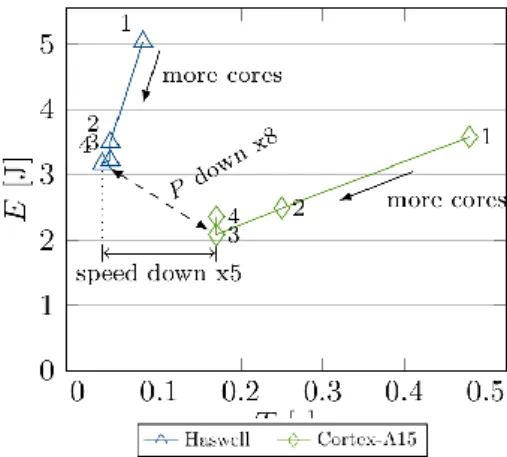
In the following we show how to deduce a model that predicts the energy to solution E for a given CFD code. This model hence is simply an equation, that determines E when running the application with certain run time parameters. This model is given in Equation (1). Its construction requires empirical data – in this case, time and energy

E

UROPEAN

C

OMMUNITY ON

C

OMPUTATIONAL

M

ETHODS IN

A

PPLIED

S

CIENCES

measurements.

In order to deduce a model that incorporates the energy to solution as a metric for energy efficiency we consider the averaged time to solution for a time step to complete (T), the averaged power dissipation during that time (P), and the resulting energy to solution (E). For this type of application once a problem is big enough to saturate the memory interface its wall clock time can be used to make predictions for other problem sizes because the time to solution is expected to behave as

T(N) = (N / Nmeasured)Tmeasured. All three T, P and thus E are then functions of the number of used cores, k. Additionally, we introduce variables ΔT for the total decrease in wall clock time and ΔP for the total increase in power dissipation

ΔT = ΔT(k) = Tk-1 - Tk , ΔP = ΔP(k) = Pk - Pk-1 We summarize some of the performance measurements that lead to the performance model described in the subsequent Equation (1) for a 3D PDE solver for the simulation of global ocean circulation on two different hardware architectures: the Intel Haswell *Intel Corp 2015a; Intel Corp 2015b+ and the Cortex-A15, the CPU in an NVIDIA Tegra K1 *NVIDIA Corp 2014+ SoC, in Table 1. With these results substantiating our hypothesis

that we have in fact a memory bandwidth-bound situation here the expected solution time for this code (given the problem size and application parameters but independent from the hardware architecture) can be modeled as a super-linear function in the number of used threads with quickly decreasing slopes, that is, ΔT(k) = 0 for moderate values of k. Power on the other hand behaves more linearly: First one can notice that when leaving the idle state a comparatively large power jump occurs which can be explained with the CPU being reconnected to the system clock or in other words, with all four cores being provided with a baseline power independent of the core workload denoted by Pbase. Once at least one core is tasked with a job, i. e., k ≥ 1, the chipset baseline power is increased by an additional constant power dissipation called Psocket. Second it can be seen that ΔP is roughly 10W for Haswell and ca. 2W for Tegra K1. Based on these findings power (and therefore energy) for this application can be modeled as a simple linear function in the number of used cores:

E(k) = P(k) T(k) = (Pbase +Psocket +

kΔP) T(k) , k ≥ 1 (1)

The practical effects of this model can be understood better when the above values are displayed

differently in an energy / time chart like in Figure 2. Because of an

over-proportional power increase compared to performance increase

there is an optimal number of threads as described above: Using more than three threads is obviously not beneficial and – for one of the two hardware architectures – sometimes even comprises an energy efficiency penalty since energy to solution increases with no benefits for the execution time. For many codes this qualitative finding by simple means holds true for many different runs on many nodes of a local cluster or on a workstation offering a great source of energy savings.

Hence we propose a rigorous

performance measurement, modeling and engineering policy in the development of applied sciences codes.

2.3 TAKING CONTROL OF THE

HARDWARE TO TARGET

Let us reconsider Figure 2. Another aspect that is depicted hereis that the hardware architectures used for scientific computing are fundamentally different: The two processors used there can be both considered multi-purpose processors with one (the Cortex-A15) not originating from the field of

Table 1. Performance and power measurements and values of basic model variables

Figure 2. Energy and time to solution of a memory bandwidth-bound application on two different hardware architectures

computing. Recently a game-changing impulse regarding energy-efficient compute hardware comes from mobile/embedded computing with devices featuring a long history of being developed under one major aspect: they have had to be operated with a (limited) battery power supply. Hence as opposed to x86 and other commodity designs (with a focus on chipset compatibility and performance) the resulting energy efficiency advantage can be made accessible to the scientific community.

In our example the CFD code shows higher energy efficiency on the mobile CPU than on the commodity CPU. This is possible because comparing the respective run on the two micro architectures the power

down is larger than the speed down. Obviously this comes with a

price: the execution time is larger when using the embedded processor. This exemplifies a general problem: Energy to solution is not only barely visible to the applied sciences community but also minimizing it is not an inherent goal of what is usually done and even worse: Using the most energy-efficient hardware penalizes the user with a slowdown. We shall demonstrate how to overcome this issue by scaling such unconventional

hardware resources and numerically scale the code, see below.

However in situations when it is possible in future times energy

efficiency should be favored over performance and in this case a good

knowledge of the energy-related hardware specifics is needed. Luckily the performance modeling described in the above section offers a good way to explore these. Devices of the family used in the above benchmarks are on the march and are more and more built into servers and data centers. Normally in a local data center in future times or even now there might be a variety of types of compute nodes available to the user or a department comprises several clusters and workstations of different kind. As a basic pattern to reduce the energy footprint of applied sciences work the performance modeling allows for choosing the most energy-efficient hardware for a workload or application.

To fortify our point here we demonstrate the performance and energy efficiency on the device level for very different hardware architectures and very different types of codes in Figures 3 and 4.

The results depict two very well known but often not addressed phenomena: (1) Performance and energy efficiency are functions of device hardware and (the operational intensity of) code; and (2) the hardware ecosystem is evolving very fast over time.

For (1) consider for example the top diagram in Figure 3. The purple plot marks performance for the same ARM Cortex-A15 CPU as in Figure 2. Note that this time for a compute-bound kernel (dense matrix matrix multiply, GEMM) performance and energy efficiency are considerably higher when using commodity processors based on the x86 architecture. Hence over-generalized assumptions like ‘ARM-based devices/computers are always more energy-efficient than x86 ones’ are as wrong as they are futile. For (2) consider the bottom plot in Figure 3 where this time commodity and embedded GPUs of different hardware generations are compared. Here we examined the low power GPUs of the NVIDIA Tegra-K1 SoC *Geveler et al. 2016b+. Note how the low power GPU is able to beat desktop CPUs of their time as well as later generation desktop GPUs in terms of energy efficiency whereas same-generation compute GPUs (Tesla line) are the

Figure 3. Energy and time to solution of compute-bound basic kernels on different hardware architectures

Figure 4. Energy and time to solution for memory bandwidth-bound basic kernels on different

E

UROPEAN

C

OMMUNITY ON

C

OMPUTATIONAL

M

ETHODS IN

A

PPLIED

S

CIENCES

most energy efficient floating point accelerators of that time. For a different type of kernel the picture is changing: In the memory bandwidth -bound case in Figure 4 (as with the sparse matrix vector multiply) powering memory interfaces is much more important and thus hardware generation determines the energy-efficiency due to the enhanced memory interface of the 2015 GPU. Also the embedded GPUs are evolving and the next generations (Tegra X1 and X2) may turn this picture upside down again. Hence continuous work regarding measurement and modeling energy for application codes and available hardware is crucial and nothing should be taken as carved in stone.

Another point here is that computing is not all about CPUs and memory interfaces. A compute node in a cluster may be a complex architecture which is then aggregated into an even more complex system with communication switches, storage and control hardware. This cluster is integrated into a housing with cooling systems. All these systems drain energy for the sake of computations. Let us now take a look at the cluster level where everything is scaled up. In Figure 5 we demonstrate results from a cluster of compute nodes consisting of single Tegra K1 SoCs which combine 4 Cortex- A15 CPU cores and a low power Kepler GPU. These results show that together with energy-efficient switches we can use a number of nodes comprising the ‘unconventional’ computer hardware to be both more energy-efficient as well as faster. Hence we

can scale the energy-efficiency bonuses by embedded hardware up to a point where the resulting cluster performs faster and uses less energy at the same time as compared to single commodity devices. It is very important to

understand that this is only possible by developing numerics

that fit to the underlying hardware and are able to be scaled numerically and hardware efficiency-wisely to reach that point.

Another aspect concerning hardware is that the energy revolution is not all about energy efficiency. Up to now we basically proposed to reduce energy by enhancing hardware or software energy efficiency on the scale of our own codes and hardware devices. This does not ease the problem that even with optimal devices the problem of too few energy supplies for future computing cannot be resolved – at least not with ‘standard’ computers. This kind of thinking led us to a system integration project where we built a

compute-cluster alongside with its power supply by renewable energies, see Figure 6 for snapshots

of the ICARUS project site *Geveler and Turek 2016+. This prototypical data and compute center comprises a great deal of theoretical peak performance (around 20 TFlop/s) provided by 60 Tegra K1 processors that all have a low power GPU on the SoC. By applying a 45 m2 solar farm offering a 8 kWp power source alongside with a Lithium-Ion battery with a capacity of 8 kWh we can maintain operation of the 1 kW peak power dissipation computer even during nighttime for several hours. Even with comparatively cloudy weather and considerably large nightly workloads we can recharge the battery at day times while computing under full load. This computer has all its energy needs fed by renewables even the cooling system and it is not connected to the power grid at all.

The idea of the project is: If we cannot tackle the overall problem of energy demand increasing much faster than its supply why not build

any new needed supply directly with the system? In recent work we proved that this is possible *Geveler et al. 2016b+. With this we come back to Figure 1. Note that finally building new renewable energy sources alongside with its demand in the model used by the SIA the supply curve would be parallel to the consumption. Higher energy efficiency is still needed because renewable energy sources such as photovoltaic units impose new constraints like area or initial cost that should be minimised. Building compute centers this way we could reduce the follow-up energy cost of a computational resource to zero.

3 C

ONCLUSION

Keep in mind that the system integration described in the previous section is only possible due to simple yet very effective performance modeling which allows for choosing hardware and numerics as well as tuning them properly. Therefore hardware-oriented numerics is the central aspect here:

The approach is successful for a specific type of numerics that can be Figure 5. Energy and time to solution of a CFD application on a cluster of Tegra K1 SoCs and several workstations comprising commodity

scaled effectively i.e. numerically and in terms of hardware -and energy- efficiency. Hardware-oriented numerics therefore means:

(1) The extension of the original paradigm by the aspect of

energy-efficiency. New methods in performance modeling have to be developed and applied and energy to solution has to be internalized into tuning efforts of software on the application level.

(2) The selection of compute

hardware should be based on these models. In any decision and where

necessary energy efficiency should

be favored over raw performance

although we have shown how this can be bypassed by clustering unconventional computer hardware and enhancing scalability properties of a given code.

(3) Furthermore knowledge concerning energy efficient computing has to be spread in the applied science community. A

knowledge base should be installed that disseminates methods in power and energy measurement as well as profiling and benchmarking techniques in order to bring up sophisticated performance models for the application level, performance engineering for energy -efficiency, energy consumption of compute devices in local compute resources and energy consumption of compute clusters and whole data centers.

(4) After hardware selection many

hardware parameters have to be tuned during operation. We demonstrated how to determine an optimal number of threads for a maximum of energy efficiency. Another good example here is finding an optimal preset core frequency. Although with Dynamic Frequency Scaling modern processors show very complex behavior for different workloads and especially during runs of complex applications, in many cases one can find an optimal frequency for a certain type of applications with similar sets of measurements like in our example.

(5) Finally, the development of the ICARUS system has been accompanied by a two semesters student project where the participants actively contributed to the system design. Here they learned how to co-develop hard- and software/numerics from scratch for computations being powered by renewables and batteries starting with performance modeling and hardware details up to integrating everything into a future-proof resource. It is bringing sensitivity

for energy efficiency and consumption into the peoples’ minds which starts with being integrated into teaching which is in

the end maybe the most important thing one can do.

A

CKNOWLEDGMENTS

ICARUS hardware is financed by MIWF NRW under the lead of MERCUR. This work has been supported in part by the German Research Foundation (DFG) through the Priority Program 1648 ‘Software for Exascale Computing’ (grant TU 102/48). We thank the participants of student project Modeling and Simulation 2015/16 at TU Dortmund for initial support.

R

EFERENCES

ANZT, H., AND QUINTANA-ORTÍ, E. S. 2014. Improving the energy efficiency of sparse linear system solvers on multicore and manycore systems. Phil. Trans. R. Soc. A 372, 2018. doi: 10.1098/rsta.2013.0279.

BENNER, P., EZZATTI, P., QUINTANA-ORT, E., AND REMN, A. 2013. On the impact of optimization on the time-power-energy balance of dense linear algebra factorizations. In

Algorithms and Architectures for Parallel Processing, R. Aversa, J.

Koodziej, J. Zhang, F. Amato, and G. Fortino, Eds., vol. 8286 of Lecture

Notes in Computer Science. Springer

International Publishing, 3–10. doi: 10.1007/978-3-319-03889-6 1.

FENG, W., CAMERON, K., SCOGLAND, T., AND SUBRAUMANIAM, B., 2015. Green500 list, jul. http://www. green500.org/lists/green201506. Figure 6. Snapshots of the ICARUS cluster at TU Dortmund

E

UROPEAN

C

OMMUNITY ON

C

OMPUTATIONAL

M

ETHODS IN

A

PPLIED

S

CIENCES

GEVELER, M., AND TUREK, S., 2016. ICARUS project homepage. http:// www.icarus-green-hpc.org.

GEVELER, M., RIBBROCK, D., GÖDDEKE, D., ZAJAC, P., AND TUREK, S. 2013. Towards a complete FEM–based simulation toolkit on GPUs: Unstructured grid finite element geometric multigrid solvers with strong smoothers based on sparse approximate inverses.

Computers and Fluids 80 (July), 327–

332. doi: 10.1016/ j.compfluid.2012.01.025.

GEVELER, M., REUTER, B., AIZINGER, V., GÖDDEKE, D., AND TUREK, S. 2016. Energy efficiency of the simulation of three-dimensional coastal ocean circulation on modern commodity and mobile processors – a case study based on the Haswell and Cortex-A15 microarchitectures.

Computer Science - Research and Development, 1-10 (June). doi:

10.1007/s00450-016-0324- 5.

GEVELER, M., RIBBROCK, D., DONNER, D., RUELMANN, H., H¨O PPKE, C., SCHNEIDER, D., TOMASCHEWSKI, D., AND TUREK, S. 2016. The ICARUS white paper: A scalable, energyefficient, solar-powered hpc center based on low power gpus. In Workshop on

Unconventional HPC, Springer, LNCS,

Euro-Par ’16. accepted.

HAGER, G., TREIBIG, J., HABICH, J., AND WELLEIN, G. 2014. Exploring performance and power properties of modern multicore chips via sim-ple machine models. Concurrency

and Computation: Practice and Experience. doi: 10.1002/cpe.3180.

INTEL CORP, 2015. Desktop 4th Generation Intel Core Processor Family, Desktop Intel Pentium Processor Family, and Desktop Intel Celeron© Processor Family Datasheet Volume 1 of 2. http://

www.intel. com/content/www/us/ en/processors/core/4th-gen-core-family-desktop-vol-1-datasheet. html.

INTEL CORP, 2015. Desktop 4th Generation Intel Core Processor Family, Desktop Intel Pentium Processor Family, and Desktop Intel Celeron© Processor Family Datasheet Volume 2 of 2. http:// www.intel. com/content/www/us/ en/processors/core/ 4th-gen-core-family-desktop-vol-2-datasheet. html.

LAWRENCE BERKELEY NATIONAL LABORATORY, 2006. Highperfor-mance buildings for high-tech industries: Data centers. http:// hightech.lbl.gov/datacenters.htm.

MALAS, T. M., HAGER, G., LTAIEF, H., AND KEYES, D. E. 2014. Towards energy efficiency and maximum computational intensity for stencil algorithms using wavefront diamond temporal blocking. CoRR abs/1410.5561. http://arxiv.org/ abs/1410.5561.

MEUER, H., STROHMEIER, E., DONGARRA, J., SIMON, H., AND MEUER, M., 2015. Top500 List, jul. http://top500.org/ lists/2015/06/.

NVIDIA CORP, 2014. NVIDIA Jetson TK1 Development Kit - Bringing GPU -accelerated computing to Embedded Systems. http:// developer.download.nvidia.com/ embedded/jetson/TK1/docs/ Jetson_platform_brief_May2014.pdf SCHÄPPI, B., PRZYWARA, B., BELLOSA, F., BOGNER, T., WEEREN, S., HARRISON, R., AND ANGLADE, A. 2009. Energy efficient servers in Europe – energy consumption, saving potentials and measures to support market development for energy efficient solutions. Tech. rep., Intelligent Energy Europe

Project, June.

SIA, 2015. Rebooting the it revolution: A call to action, sept. http://www.semiconductors. org/ clientuploads/Resources/RITR% 20WEB% 20version%20FINAL.pdf.

TUREK, S., BECKER, C., AND KILIAN, S. 2006. Hardware–oriented numerics and concepts for PDE soft-ware. Future Generation Computer

Systems 22, 1–2, 217–238. doi:10.1016/j.future.2003.09.007.

TUREK, S., GÖDDEKE, D., BECKER, C., BUIJSSEN, S., AND WOBKER, H. 2010. FEAST — realisation of hardware–oriented numerics for HPC simulations with finite elements. Concurrency and Computation: Practice and Experience 6 (May), 2247–2265.

Special Issue Proceedings of ISC 2008. doi:10.1002/cpe.1584.

M

ARKUS

G

EVELER

TU

D

ORTMUND,

G

ERMANY MARKUS.GEVELER@MATH.TU-DORTMUND.DE

S

TEFAN

T

UREK

TU

D

ORTMUND,

G

ERMANY TURE@FEATFLOW.DE

COMMUNICATED BY OLIVIER ALLIX, CHAIRMAN OF THE ECCOMAS TECHNICAL COMMITTEE "COMPUTATIONAL SOLID AND STRUCTURAL MECHANICS"

T

HE

V

IRTUAL

E

LEMENT

M

ETHOD:

A

N

EW

P

ARADIGM

F

OR

T

HE

A

PPROXIMATION

O

F

P

ARTIAL

D

IFFERENTIAL

E

QUATION

P

ROBLEMS

Foreword. The present note is not intended to provide an exhaustive account of the numerous research directions, results and applications developed by the various groups working on the Virtual Element Method. Instead, our aim is to concisely present the basic ideas of the method, and to mention only a few aspects which highlight the potential and the flexibility of this innovative approach.

The Virtual Element Method (VEM) is a new technology for the approximation of partial differential equation problems. VEM was born in 2012, see *6+, as an evolution of modern mimetic schemes (see for instance *14, 5, 12+), which share the same variational background of the Finite Element Method (FEM). The initial motivation of VEM is the need to construct an accurate Galerkin scheme with the following two properties.

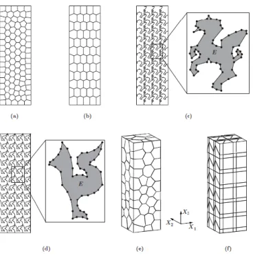
 The flexibility to deal with highly general polygonal/polyhedral meshes, including “hanging vertexes” and non-convex shapes. A couple of instances are depicted in Figures 1 and 2.

 The conformity of the method, i.e. the property to build an approximated solution which shares the same “natural” regularity as the analytical solution of the problem. In many interesting cases, this means that the discrete solution is continuous

across adjacent elements.

When confining to polynomial local approximation, the two features above are severely conflicting, thus making the method design extremely difficult. The virtual element method overcomes the trouble by abandoning the local

polynomial approximation concept,

and use, instead, approximating functions which are solutions to suitable local partial differential equations (of course, connected with the original problem to solve). Therefore, in general, the discrete functions are not known pointwise, but a limited information of them are at disposal. However, the available information is sufficient for the formation of the stiffness matrix and the right-hand side: this can be accomplished by designing a weakly (not strongly!) consistent scheme;

strong consistency is imposed only for polynomials up to a suitable degree, but not for the whole approximating space. We remark that the strong consistency on polynomials essentially implies the fulfilment of the patch test relevant to the specific problem at hand.

In addition to the features mentioned above, we present some other interesting properties that make the virtual element method an attracting methodology:

 An accurate description of possible discontinuities in the data, especially when they occur in accordance with complex patterns (e.g. in reservoir simulation or crack propagation problem).

 For mesh adaptivity, the possibility to refine without the need to avoid hanging nodes/edges allows for more efficient refinement strategies. Moreover using polygonal/polyhedral meshes allow interesting de-refinement procedures in which groups of elements are coalesced into single ones.

E

UROPEAN

C

OMMUNITY ON

C

OMPUTATIONAL

M

ETHODS IN

A

PPLIED

S

CIENCES

• In topology optimization, the use of polygonal/polyhedral meshes may alleviate phenomena connected to preferred geometric directions, inevitably occurring with low-sided polygons/ polyhedra.

 Surprisingly, the virtual element method can easily handle approximating spaces with high

order regularity, such as C1,C2 or

more. This property makes VEM very attractive when dealing with high-order partial differential equations, such as the Kirchhoff plate problem.

 VEM is generally more robust than traditional FEM with respect to mesh distortion or degeneration.  For constrained problems, such as

incompressible elasticity, the flexibility of VEM to choose the approximating spaces, opens the way to new schemes, where the constraint is exactly satisfied. In the FEM framework, instead, the exact satisfaction of the constraints is typically difficult to reach.

Before presenting a concise but “precise” description of the method, we state that despite VEM was born very recently, a significant number of contributions have already appeared in literature. From the theoretical side, the analysis of VEM applied to several linear model problems have been developed. We cite here the works: *6, 9, 13, 17+. For nonlinear problems, the available theoretical results are still very limited, see *15, 2+. Regarding the application side, VEM is experiencing a growing interest from the engineering community. We mention a few (non exhaustive) list of applications where the VEM approach has shown or is showing promising results:

 The Stokes problem. In fluid-dynamics applications, the flexibility of VEM has been exploited to develop a highly regular (i.e. C1) scheme based on a

stream function formulation of the

Stokes problem, see *1+. A different approach has been followed in *8+, where the non-polynomial character of VEM is

used to design new exactly

divergence-free schemes.

 2D and 3D elasticity problems. The classical elasticity problem, in the framework of the infinitesimal theory, has been addressed in the works *7, 16, 3+, among others. Also in this case, VEM has proved to be a competitive alternative to the more traditional FEM procedures, especially when the problem requires a particularly flexible management of the geometry description.

 Fracture problems. For some fracture problems arising from reservoir applications, the VEM approach has been developed in *10+.

 Contact problems. In *20+, VEM is proved to provide an interesting methodology for contact problems. Here, the VEM ability to deal with glued unrelated meshes is greatly beneficial.

 Inelastic problems. In the papers *15, 4+ VEMs are used for the analysis for inelastic phenomena Figure 1. Example of 2D mesh that can be used

in connection with VEM (courtesy of A. Russo).

Figure 2. Example of 2D and 3D meshes that can be used in connection with VEM (courtesy of G.H. Paulino).

(such as plasticity, shape memory alloys and viscoelastic problems), modelled by the generalized standard material theory (see *11+, for example). Among other results, it is proved that the VEM approach can be interfaced with a standard numerical treatment of the evolution flow rule governing the internal and history variables. Therefore, most of the technology already developed in the FEM framework for such problems, can be easily reused by the new paradigm.

 Phase separation problems (the

Cahn-Hilliard equation). For phase

separation problems modelled by the Cahn-Hilliard equation, the VEM philosophy has been studied in *2+, where the ability of designing highly regular (i.e. C1) schemes is exploited.

 The Helmholtz problem. For the 2D Helmholtz equation with impedance boundary conditions, an application of VEM can be found in *18+.

However, we remark that this new technology has been tested essentially on academic, though interesting, problems. So far, VEM has displayed a number of surprisingly interesting features. It is

now time to inject efforts towards the development, the assessment and the validation of the VEM paradigm when applied to real-life problems.

A C

ONCISE

P

RESENTATION

O

F

T

HE

V

IRTUAL

E

LEMENT

M

ETHOD

We here present the basic idea of the virtual element method by considering a very simple model problem: the Poisson problem. Accordingly, we are asked to find a function u : Ω → ℝ, solution to the following problem:

- Δu = f in Ω, u = 0 on Ω. (1) It is well-known that a variation formulation of problem (1) reads:

Find u V such that:

α(u, υ) = (f, υ) υ V, (2) where V is the trial/test space,

The virtual element method falls in the category of Galerkin schemes for the approximation of the solution to problem (2):

Find uh Vh such that:

ah(uh, υh) = Fh(υh) υh Vh. (3) Here above, Vh is the finite dimensional approximating space tailored to a given mesh Ωh made by polygons E, ah(,) is the discrete bilinear form (leading to the method stiffness matrix), and Fh() is the discrete loading term.

D

EFINITION

O

F

T

HE

A

PPROXIMATING

S

PACE

V

h

The first problem we have to face is to find a finite dimensional space

Vh V, tailored to the mesh Ωh. Similarly to the finite element approach, we would like to define

Vh by gluing local approximation spaces VE , one per each polygon E Ωh. The polynomial character of a typical υE VE is abandoned, and υE is instead defined as the solution of a particular partial differential equation problem in E. More precisely, we take

VE = {υE :ΔυE =0, υE|E C0_(E),

υE linear on every edge e E }. (4)

Therefore, the local degrees of freedom can be chosen as the vertex values of VE. We notice that it obviously holds ℙ1(E)  VE, where ℙ1(E) denotes the space of linear polynomials defined on E. This property is one of the roots for the consistency of the method, and ultimately for the satisfaction of the

patch test.

The approximating space Vh is then built by gluing together the local spaces VE. Therefore, the global degrees of freedom are the values at the interior vertexes of the mesh Ωh. We also notice that, when Ωh is a triangular mesh, the space Vh is exactly the same as for the standard linear triangular finite element method.

D

EFINITION

O

F

T

HE

D

ISCRETE

B

ILINEAR

F

ORM

a

h

(,)

At a first glance, definition (4) seems to hide an insurmountable obstacle: in general, the functions υE VE are

not explicitly known, and of course, nor are the elements of a basis, say

,φi-. The observation that the local stiffness matrix is formed by the terms , seems to put

an end to the utility of definition (4) in designing a Galerkin scheme. We now show how to overcome this trouble.

First Step. For each polygon E, we

introduce a projection operator ΠE : VE → ℙ1(E), thus taking values on the linear polynomial space. More precisely, we set:

ΠEυE ℙ1(E):aE (ΠEυE ,q) = aE(υE ,q) q ℙ1(E) ; (5)

where αE(,) denotes the energy contribution computed on the polygon E Th. We notice that:

E

UROPEAN

C

OMMUNITY ON

C

OMPUTATIONAL

M

ETHODS IN

A

PPLIED

S

CIENCES

aE(ΠEυE , q) = aE(υE , q) q ℙ1(E) is a linear system of three equations in the unknowns, since dim (ℙ1(E)) = 3. However, taking q = 1 gives 0 = 0, which means that there are only two independent equations. As a consequence, we need to add another independent equation to uniquely define ΠEυE ℙ1(E): this is indeed embodied by the condition

We also notice that ΠE is nothing

but the orthogonal projection

operator onto the linear polynomials, with respect to the bilinear form aE(,). But the crucial remark is that ΠEυE is computable

for every υE, despite υE is not

explicitly known, in general. For the

details of such a fundamental property we refer to *6+.

Second Step. Given uE , υE VE, one can now write uE = ΠE uE + ( I - ΠE)

uE and υE = ΠE υE + ( I - ΠE) υE , and notice that they are orthogonal decompositions with respect to the bilinear form aE(,). As a consequence, it holds aE (uE , υE ) =

aE (ΠE uE , ΠE υE ) + aE (( I - ΠE) uE , ( I - ΠE) υE ). The first term at the right-hand side is computable, hence it can be retained as it is to design a Galerkin scheme. Instead, the second term at the right-hand side cannot be computed, hence it needs to be properly modified. The modification should mimic the original term as much as possible, but it must be computable for every

υE VE. In particular, it must scale, with respect to the size of the polygon E, as aE(,) scales. A typical choice stems from the introduction of the bilinear form

(6)

Then, we can set

(7)

which turns out to be computable for every uE , υE VE. We notice that the form in (7) is strongly consistent on linear polynomials, and it scales as the original bilinear form. These two features are indeed sufficient to design an effective method, and different stabilisation terms sE might be accordingly designed.

Third Step. The global bilinear form ah_{(,) is simply defined by gluing the} local contributions:

where uE =uh|E and υE =υh|E . (8)

D

EFINITION

O

F

T

HE

R

IGHT

-H

AND

S

IDE

Fh

()

For the approximation of the right-hand side

we first define a piecewise constant approximation Then, we set

(9)

where

and n(E) is the number of vertexes in E.

R

EFERENCES

*1+ P. F. Antonietti, L. Beirão da Veiga, D. Mora, and M. Verani,

A stream virtual element formulation of the Stokes problem on polygonal meshes,

SIAM J. Numer. Anal. 52 (2014), no. 1, 386–404. MR 3164557

*2+ P. F. Antonietti, L. Beirão da Veiga, S. Scacchi, and M. Verani, A C1 virtual element method for the Cahn–Hilliard equation with polygonal meshes, SIAM Journal on

Numerical Analysis 54 (2016), no. 1, 34–56.

*3+ E. Artioli, L. Beirão Da Veiga, C. Lovadina, and E. Sacco,

Arbitrary order 2D virtual elements for polygonal meshes: Part I, elastic problem,

in preparation.

*4+ Arbitrary order 2D virtual

elements for polygonal meshes: Part II, inelastic problems, in preparation.

*5+ L. Beirão da Veiga, K. Lipnikov, and G. Manzini, The mimetic

finite difference method for elliptic problems, Springer, series MS&A (vol. 11), 2014. *6+ L. Beirão da Veiga, F. Brezzi, A.

Cangiani, G. Manzini, L. D. Marini, and A. Russo, Basic

principles of virtual element methods, Math. Models Methods Appl. Sci. 23 (2013), no. 1, 199–214. MR 2997471 *7+ L. Beirão da Veiga, F. Brezzi,