Efficient algorithms to solve scheduling problems with a variety of optimization criteria

(1)

Efficient algorithms to solve scheduling problems

with a variety of optimization criteria

Thèse Hamed Fahimi Doctorat en informatique Philosophiæ doctor (Ph.D.) Québec, Canada © Hamed Fahimi, 2016

(2)

Efficient algorithms to solve scheduling problems

with a variety of optimization criteria

Thèse

Hamed Fahimi

Sous la direction de:

(3)

Résumé

La programmation par contraintes est une technique puissante pour résoudre, entre autres, des pro-blèmes d'ordonnancement de grande envergure. L'ordonnancement vise à allouer dans le temps des tâches à des ressources. Lors de son exécution, une tâche consomme une ressource à un taux constant. Généralement, on cherche à optimiser une fonction objectif telle la durée totale d'un ordonnancement. Résoudre un problème d'ordonnancement signifie trouver quand chaque tâche doit débuter et quelle ressource doit l'exécuter. La plupart des problèmes d'ordonnancement sont NP-Difficiles. Conséquem-ment, il n'existe aucun algorithme connu capable de les résoudre en temps polynomial. Cependant, il existe des spécialisations aux problèmes d'ordonnancement qui ne sont pas NP-Complet. Ces pro-blèmes peuvent être résolus en temps polynomial en utilisant des algorithmes qui leur sont propres. Notre objectif est d'explorer ces algorithmes d'ordonnancement dans plusieurs contextes variés. Les techniques de filtrage ont beaucoup évolué dans les dernières années en ordonnancement basé sur les contraintes. La proéminence des algorithmes de filtrage repose sur leur habilité à réduire l'arbre de re-cherche en excluant les valeurs des domaines qui ne participent pas à des solutions au problème. Nous proposons des améliorations et présentons des algorithmes de filtrage plus efficaces pour résoudre des problèmes classiques d'ordonnancement. De plus, nous présentons des adaptations de techniques de filtrage pour le cas où les tâches peuvent être retardées. Nous considérons aussi différentes proprié-tés de problèmes industriels et résolvons plus efficacement des problèmes où le critère d'optimisation n'est pas nécessairement le moment où la dernière tâche se termine. Par exemple, nous présentons des algorithmes à temps polynomial pour le cas où la quantité de ressources fluctue dans le temps, ou quand le coût d'exécuter une tâche au temps t dépend de t.

(4)

Abstract

Constraint programming is a powerful methodology to solve large scale and practical scheduling problems. Resource-constrained scheduling deals with temporal allocation of a variety of tasks to a set of resources, where the tasks consume a certain amount of resource during their execution. Ordinarily, a desired objective function such as the total length of a feasible schedule, called the makespan, is optimized in scheduling problems. Solving the scheduling problem is equivalent to finding out when each task starts and which resource executes it. In general, the scheduling problems are NP-Hard. Consequently, there exists no known algorithm that can solve the problem by executing a polynomial number of instructions. Nonetheless, there exist specializations for scheduling problems that are not NP-Complete. Such problems can be solved in polynomial time using dedicated algorithms. We tackle such algorithms for scheduling problems in a variety of contexts. Filtering techniques are being developed and improved over the past years in constraint-based scheduling. The prominency of filtering algorithms lies on their power to shrink the search tree by excluding values from the domains which do not yield a feasible solution. We propose improvements and present faster filtering algorithms for classical scheduling problems. Furthermore, we establish the adaptions of filtering techniques to the case that the tasks can be delayed. We also consider distinct properties of industrial scheduling problems and solve more efficiently the scheduling problems whose optimization criteria is not necessarily the makespan. For instance, we present polynomial time algorithms for the case that the amount of available resources fluctuates over time, or when the cost of executing a task at time t is dependent on t.

(5)

3 Filtering algorithms for the disjunctive and cumulative constraints 24 3.1 Overload Checking . . . 25 3.2 Time-Tabling . . . 28 3.3 Edge-Finding . . . 29 3.3.1 (Θ − Λ)L−tree . . . 31 3.4 Extended-Edge-Finding. . . 32 3.5 Not-First/Not-Last . . . 33 3.6 Energetic Reasoning . . . 34 3.7 Detectable Precedences . . . 35 3.8 Precedence Graph . . . 35

3.9 Combination of filtering techniques . . . 36

3.10 Filtering techniques in the state of the art schedulers . . . 36

4 Linear time Algorithms for Disjunctive constraint 38 4.1 Preliminaries . . . 39

4.1.1 Union-Find . . . 39

4.2 Time-Tabling . . . 40

4.3 The Time Line Data Structure . . . 42

4.4 Overload Checking . . . 45

4.5 Detectable Precedences . . . 45

4.6 Experimental Results . . . 47

Two sorting algorithms . . . 48

Filtering algorithms. . . 50

4.7 Minimizing maximum lateness and total delay . . . 50

4.8 Conclusion . . . 52

5 Overload Checking and Edge-Finding for Robust Cumulative Scheduling 53 5.1 Preliminaries and the general framework . . . 53

5.1.1 Robust cumulative constraint. . . 54

5.2 Robust Overload Checking . . . 55

5.2.1 The general form of robust Overload Checking rule . . . 55

5.2.2 Robust earliest energy envelope . . . 56

5.2.3 Robust Overload Checking rule in terms of robust energy envelope. . . . 56

5.2.4 Θr L−tree . . . 57

5.2.5 Robust Overload Checking algorithm . . . 58

5.3 Robust Edge-Finding . . . 59

5.3.1 Filtering the earliest starting times . . . 61

Robust Edge-Finding rule for filtering the earliest starting times . . . 61

Robust Λ−earliest energy envelope . . . 62

(Θ − Λ)r L−tree . . . 62

Robust Edge-Finding algorithm for filtering the earliest starting times . . 63

5.3.2 Filtering the latest completion times . . . 71

Robust Edge-Finding rules for filtering the latest completion times . . . . 71

(7)

Robust Λ−latest energy envelope . . . 73

(Θ − Λ)r_U−tree . . . 73

Robust Edge-Finding algorithm for filtering the latest completion times . 75 5.4 Experiments . . . 82

6 Variants of Multi-Resource Scheduling Problems with Equal Processing Times 85 6.1 Variety of machine numbers through the time . . . 86

6.2 General Objective Function . . . 88

6.3 Scheduling problems with monotonic objective functions . . . 89

6.4 Scheduling problems with periodic objective functions . . . 90

6.4.1 Scheduling problem as a network flow . . . 90

6.4.2 Periodic objective function formulated as a network flow . . . 92

6.5 Minimizing maximum lateness . . . 96

Conclusion 97

(8)

List of Tables

2.1 Resource environment possibilities depending on the value of α. . . 16

2.2 Task possibilities depending on the value of β.. . . 16

2.3 Objective possibilities depending on the value of γ. . . 16

3.1 A set of tasks for which neither Overload Checking fails, nor is there a feasible solution. 25

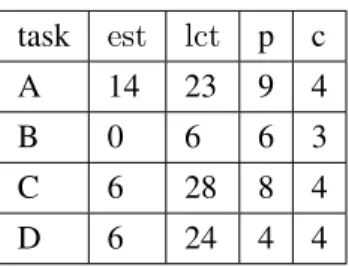
3.2 The information of a set of tasks I = {A, B, C, D} with a resource of capacity C = 3. 32

4.1 The information of a set of tasks I = {A, B, C}. . . 42

4.2 Comparison of Θ-tree and time line. . . 43

4.3 Parameters of the tasks used to illustrate the scheduling process on the time line.. . . 44

4.4 Open-shop with n jobs and m tasks per job. Ratio of the cumulative number of back-tracks between all instances of size n × m after 10 minutes of computations. OC: our Overload Checking vs. Vilím’s. DP: our Detectable Precedences vs Vilím’s. TT: Our

Time-Tabling vs Ouellet et al. All algorithms use insertion sort.. . . 51

4.5 Job-shop with n jobs and m tasks per job. Ratio of the cumulative number of back-tracks between all instances of size n × m after 10 minutes of computations. OC: our Overload Checking vs. Vilím’s. DP: our Detectable Precedences vs Vilím’s. TT: Our

Time-Tabling vs Ouellet et al. All algorithms use insertion sort.. . . 51

4.6 Random instances with n tasks. Times are reported in milliseconds. Algorithms im-plementing the same filtering technique lead to the same number of backtracks (bt).

TT: Θ−tree, TL: time line, UF:Union-Find data structure. . . 51

5.1 A set of tasks I = {A, B, C, D, E} to execute on a resource of capacity C = 4. The Overload Checking fails according to (5.7) for Θ = {A, B, C, D} ⊆ I, Θ0 =

{A0_{, C}0_{} and Θ}1_{= {B}1_{, D}1_}. _{. . . .} ₅₅

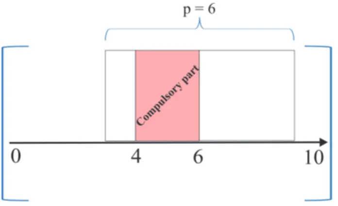
5.2 A set of tasks I = {A, B, C, D} to execute on a resource of capacity C = 7. . . 62

5.3 The prec array which is obtained after the execution of the algorithm 11 on the instance

of example 5.3.1 . . . 67

5.4 The prec array which is obtained after the execution of the algorithm 15 on the instance

of example 5.3.2 . . . 78

6.1 Summary of the contributions mentioned in this thesis. NA stands for no previously

(9)

List of Figures

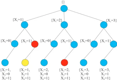
1.1 The search tree corresponding to a CSP with X = {X1, X2, X3}, dom(X1) = {1, 2, 3}, dom(X2) =

{0, 1}, dom(X3) = {1} and C : X1 ≥ 2X2+ X3. At the red node, the search

back-tracks, as the assignments on the path to that node violate the constraint C. The yellow node indicates an unvisited node, due to the occurrence of a backtrack on the branch

connection leading to that node. . . 9

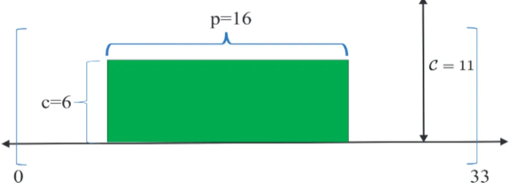
2.1 The components of a task A with estA= 0, lctA= 33, pA= 16, cA= 6, carrying out on a resource with C = 11. A has eA= 6 × 16 = 96 units of energy. . . 13

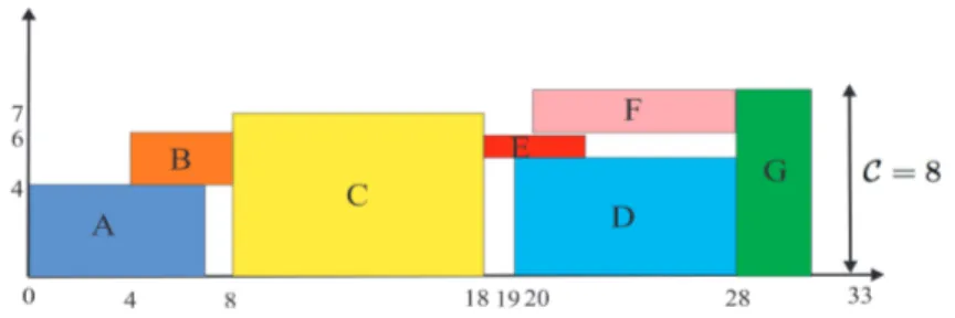
2.2 For the set of tasks I= {A,B,C,D,E,F,G} which must execute on a resource of ca-pacity C = 8 the assignment (sA, sB, sC, sD, sE, sF, sG) = (0, 4, 8, 19, 18, 20, 28) provides a valid schedule, where dom(sA) = [0, 10), dom(sB) = [2, 8), dom(sC) = [5, 21), dom(sD) = [15, 33), dom(sE) = [13, 26), dom(sF) = [17, 31), dom(sG) = [20, 33). . . 14

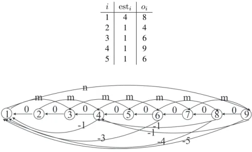
2.3 The scheduling graph with five tasks with processing times p = 2. . . 22

2.4 A network flow and a residual network flow. . . 23

3.1 Overload Checking triggers a failure for Θ = {A, B, C, D}. . . 25

3.2 The cumulative ΘL−tree corresponding to I = {A, B, C, D} with a resource of ca-pacity C = 3. . . 27

3.3 The compulsory part of the task A with estA= 0, lctA= 10, pA= 6 is [4,6). . . 28

3.4 The precedence Θ1 = {B, E} ≺ D gives rise to filtering estD = 20 and the prece-dences D ≺ Θ2 = {A} and B ≺ Θ3 = {A, D, E} give rise to lctD = 40, lctB = 25. 30 3.5 Detectable precedences detects A C, B C, A D, B D for the tasks of table 3.5.. . . 35

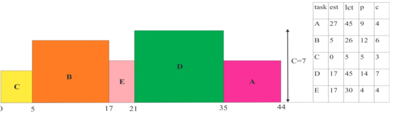
3.6 The appropriate sequence for the DISJUNCTIVEconstraint, presented in Vilím’s the-sis [88], which achieves the fixpoint . . . 37

4.1 A trace of Time-Tabling algorithm for the tasks of table 4.1. . . 42

4.2 The tasks Iect = {1, 2, 3, 4} and the visual representation of a solution to the DIS -JUNCTIVEconstraint. The algorithm Detectable Precedences prunes the earliest start-ing times est0₃= 19 and est0₄ = 13 . . . 48

4.3 Implementing insertion sort (x axis) and quick sort (y axis) when the state of the art is used for the instances of open shop problem. The figures represent the logarithmic based scale of the number of backtracks occurred within 10 minutes. OC stands for Overload Checking, DP stands for Detectable Precedences and TT stands for Time-Tabling. . . 49

(10)

4.4 Implementing insertion sort (x axis) and quick sort (y axis) when our algorithms are used for the instances of open shop problem. The figures represent the logarithmic based scale of the number of backtracks occurred within 10 minutes. OC stands for Overload Checking, DP stands for Detectable Precedences and TT stands for

Time-Tabling. . . 49

5.1 In the picture (a), C0 and C1 are scheduled in the Θr_L−tree. The coloured nodes in blue represent the affected nodes during the update of the tree. In this case, Θ0 = {C0_{} and Θ}1 _{= {C}1_{}. In the picture (b), A}0 _{is scheduled in the Θ}r

L−tree, but not

A1. In this case, Θ0 = {C0, A0} and Θ1 _{= {C}1_{}. In the picture (c), A}1 _{and D}

are scheduled. In this case, Θ0 = {C0, A0, D0} and Θ1 _{= {C}1_{, A}1_{}. Picture (d)}

represents the status of the Θr_L−tree when processing t = 25. Since Env2(Θ0, Θ1) =

Env2_root= 102 > 4 · 25 = 100 the Overload Checking triggers a failure. . . 60

5.2 In the picture (a), the algorithm starts with a full (Θ − Λ)r_L−tree. In the picture (b), C1 gets unscheduled from Θ1 and scheduled in Λ1. The modifications to Θ and Λ sets are respectively coloured in green and blue. In the picture (c), C0is unscheduled from Θ0 and scheduled in Λ0. In the picture (d) after C1 is found as the responsible tasks, it gets unscheduled from Λ1. In the picture (e), D1 gets unscheduled from Θ1

and scheduled in Λ1. . . 66

5.3 The state of Θcr_L−tree in the iteration that estC gets adjusted. The blue arrows show

the path which is traversed by the algorithm 12. This algorithm locates the yellow node. The algorithm 13 starts from the yellow node and the green arrows show the

path traversed by this algorithm to the root. . . 70

5.4 In the figure a, the algorithm starts with a full (Θ − Λ)r_U−tree. In the figure b, A gets unscheduled from Θ and scheduled in Λ. In the figure c, A1and then A0are detected

as responsible tasks and get unscheduled. In the figure d, B is unscheduled. . . 77

5.5 The logarithmic scale graphs as the results of running Time-Tabling and Overload Checking (denoted OC-TT) or Time-Tabling and Edge-Finding(denoted EF-TT) with lexicographic heuristics in terms of backtrack numbers as well as elapsed times. The horizontal axis corresponds to the Time-Tabling and the vertical axis corresponds to

Overload Checking or Edge-Finding. . . 82

5.6 The logarithmic scale graphs as the results of running Time-Tabling and Overload Checking (denoted OC-TT) or Time-Tabling and Edge-Finding(denoted EF-TT) with impact based search heuristics in terms of backtrack numbers as well as elapsed times. The horizontal axis corresponds to the Time-Tabling and the vertical axis corresponds

to Overload Checking or Edge-Finding. . . 83

5.7 The logarithmic scale graphs as the results of running Time-Tabling and Overload Checking (denoted OC-TT) or Time-Tabling and Edge-Finding(denoted EF-TT) with domoverwdeg heuristics in terms of backtrack numbers as well as elapsed times. The horizontal axis corresponds to the Time-Tabling and the vertical axis corresponds to

Overload Checking or Edge-Finding. . . 84

6.1 A trace of the algorithm 19, where p = 2 and T = [(1, 3), (3, 5), (4, 2), (6, 6)]. The

sequences T0 and T00are constructed, as represented at lines (b) and (c). . . 88

6.2 A network flow with 5 tasks. The cost on the forward, backward, and null edges are written in black. These edges have unlimited capacities. The capacities of the nodes

(11)

6.3 The compressed version of the graph on Figure 6.2. The numbers over the edges

(12)

Aknowledgments

During the preparation of this work, I had the pleasure to greatly benefit from thoughtful comments given by my supervisor Claude-Guy Quimper, a source of acumen and encouragement, who accom-panied the development of this work with numerous advices for improvements and shared his useful insights in this effort. This work would have not been in such a state if he did not provide me with his fruitful cooperation.

The author is also indebted to the community members of this dissertation, François Laviolette and Jonathan Gaudreault for supporting this work by many inspired discussions, not to mention Thierry Petit and Richard Khoury for reading and commenting my manuscript as well as evaluating the de-fence.

Thanks are also due to anonymous reviewers for their useful recommendations to improve the manuscripts before publication.

I also wish to acknowledge Giovanni Won Dias Baldini Victoret for his assistance in the experimental results of chapter 4 and Alban Derrien for providing his implementation of the Time-Tabling algorithm for the results of chapter 5.

(13)

Introduction

Scheduling is an occasionally used concept to which we are accustomed in our daily life, notwith-standing keeping a standard definition for that is often overlooked. Normally, we desire to plan the activities that we are engaged in beforehand for purposes such as time-saving, reducing cost charges, etc. For instance, suppose you are invited to attend the graduation ceremony of a group of students in the school, which is scheduled to start at a specified date. The place where the party takes place is located in downtown and you have to arrange for your departure in accordance with the public trans-portation schedule so that you arrive to the party on time. Such an occasion simply demonstrates a scheduling problem for which you need to care for two schedules, the ceremony as well as the public transportation, and these schedules are planned in advance.

Since the late 1950’s and early 1960’s scheduling problems have attracted a large amount of re-search [7, 93]. Covered by a wide variety of disciplines such as computer science (CS), artificial Intelligence (AI), operational research (OR), engineering, manufacturing, management, maintenance, etc., scheduling problems are mostly known as an interdisciplinary field of study, as they arise in numerous application settings in the real-world.

The general class of scheduling problems that we consider in this dissertation involves a group of activities to be carried out over a set of resources. The activities require certain amounts of resources to process. The activities and resources can have different interpretations, depending on the context. Moreover, most of the scheduling problems are optimization problems. That is, there is a desired objective to be attained, such as minimizing the duration of the schedule, minimizing the costs, max-imizing the profits, etc. Frequently, there are given precedences among the activities, prescribing the order in which they must be processed. The basic form of a schedule usually establishes the dates at which the activities should start such that the precedence and the alternative constraints hold and the objective function is optimized. Providing such dates to acquire a valid schedule for the activities is equivalent to finding a solution for the problem. This framework for the scheduling problems is expressive enough to capture dozens of features which arise in practice.

The input size of the general scheduling problems is typically proportional to the number of activities, the number of resources and the number of bits to represent the largest integer among the components of an activity. Unfortunately, the problem of solving most of the scheduling problems is NP-hard [29]. In fact, not only solving, but also verifying whether a feasible solution exists can take exponential

(14)

effort. That is why relatively less attempts have been made to achieve polynomial time algorithms for the scheduling problems, thus far.

In the literature, there are a variety of areas of general methods used to solve scheduling problems such as MIP (mixed integer programming), satisfiability testing (SAT), logic-based Benders decomposition (LBBD) [36,38] and constraint programming (CP). We focus on the latter method. Constraint pro-gramming is a generic purpose paradigm to solve combinatorial problems by interpreting them in terms of constraints. A typical constraint satisfaction problem (CSP) consists of a set of decision vari-ables, to each member of which a domain is associated. The domain includes the valid values that are assignable to the variables. Furthermore, a set of constraints that circumscribe the decision variables are established and a single objective function is to be optimized. Many problems can be presented in terms of constraints. Furthermore, many disciplines such as OR and AI, have developed methods for satisfying constraints. In particular, constraint-based scheduling provides powerful search strategies to solve scheduling problems, by taking advantage of constraint programming. Among the successful application areas of constraint programming are the cumulative and disjunctive scheduling. Cumula-tive scheduling differs from disjuncCumula-tive scheduling in the sense that in cumulaCumula-tive scheduling several activities are allowed to run simultaneously. Each activity consumes a certain amount of resource, and the CUMULATIVE constraint ensures that the accumulation of resource usage by the activities

underway at any time does not overflow the resource. In the disjunctive scheduling no more than one activity can execute on a resource and the DISJUNCTIVE constraint ensures that the activities do not overlap at any time.

The main goal of this dissertation is to address special structures of the scheduling problems en-countered in the industry, from a constraint-based viewpoint. Furthermore, we aim at tackling distinct properties of industrial scheduling problems with different objective functions that can be encountered in practical applications. Constraints can be used to encode all sort of these problems.

The domains of variables in a CSP include values which are not consistent with some constraints of the problem. Removing all inconsistencies from the domain of variables with respect to the CU

-MULATIVEconstraint is NP-Hard. However, several rules are proposed which can partially remove

inconsistencies in polynomial time. The scheduling problems that we consider to a great extent rely on a problem solving paradigm from constraint programming which is called constraint propagation. This method is a reduction technique which detects inconsistencies through the repetitive analysis of the variables and makes the problem simpler to solve. The constraint propagation process uses several filtering algorithms. These algorithms discover time zones in which the activities cannot start. Dis-covering such time zones prevent the solver from exploring some portions of the search space where no feasible solutions lie. Since constraint programming is based upon filtering algorithms, devising efficient algorithms is essential and this objective has captured the interest of many researchers in the CP community. This dissertation makes contributions to this research area by developing efficient, effective and fast filtering algorithms to solve conventional scheduling problems.

(15)

Scheduling environments are not always static in the real world and uncertainty is prevalent in this context. For instance, the operations might take longer than expected to execute, a supply chain for resources can break down and the resources becomes unavailable, etc. Such disruptions unavoidably cause delays in the activities. On the other hand, practically, it is not possible to re-compute the solutions in such cases. Therefore, it is of crucial importance to develop filtering algorithms which deal with such environments. An approach is to maintain a robust schedule that absorbs some level of unforeseen events when at most a certain number of activities are delayed. Even though this is not mentioned as an objective function, robustness is a desired criterion in a schedule.

Although the scheduling problems are NP-complete in the general form, specializations to the proper-ties of the problem can yield to problems that can be solved in polynomial time. For instance, if all the activities execute with the same duration over multiple resources, it is possible to find a solution. Fur-thermore a common objective function is to minimize the makespan, i.e. when the last task finishes. However, in practice, alternative objective functions often occur depending on the circumstances and context and yet it is essential that managers operate their business with the utmost efficiency. This dissertation particularly aims at solving more efficiently scheduling problems whose optimization cri-teria is not necessarily the makespan. For instance, we consider the cases such as when the amount of available resources fluctuates over time with respect to the activities. We also elaborate on specific objective functions that give rise to polynomiality.

The reminder of the monograph on hand consists of 7 chapters.

Chapter 1 introduces the standard CSP and the principal concepts which are relevant to the context of scheduling problems in this dissertation from a constraint based viewpoint. Moreover, a couple of overly simple, but illustrative examples are provided in order to the elucidate the notions.

Chapter 2 starts with a description of the basic entities that contribute to the construction of a gen-eral scheduling problem, including activities, resources and objective functions. After introducing these concepts, a hands-on application of this framework is described. Then, a family of well known scheduling problems are introduced. Afterwards, the scheduling problems are classified depending on the resource and activity types. Also, a systematic notation in order to refer to particular schedul-ing problems is presented. Furthermore, six global constraints which can be interpreted in terms of scheduling problems are introduced. Finally, this chapter introduces a class of particular scheduling problems which are solvable in polynomial time.

Over the past two decades, a variety of standard constraint propagation algorithms have been intro-duced for the scheduling problems. These principles are frequently employed in order to reduce the search space for the scheduling problems that are NP-hard. The basic algorithms are as follows. Over-load Checking, Time-Tabling, Edge-Finding , Extended-Edge-Finding, Not-First/Not-Last, Energetic Reasoning, Detectable Precedences and the Precedence Graph. Chapter 3 surveys these well-known filtering techniques for the DISJUNCTIVEand CUMULATIVEconstraint and introduces the state of the art algorithms.

(16)

Chapters 4, 5 and 6 compose three main chapters of this book which reflect three contributions. Chapter 4 is devoted to the DISJUNCTIVEconstraint, which is extensively used in the industrial ap-plications, such as manufacturing and supply chain management [37]. This constraint simply ensures that two activities A and B which execute on the same resource do not overlap in time. Propagation of the DISJUNCTIVEconstraint ensures that either A precedes B or B precedes A. Chapter 4 presents three new and efficient filtering algorithms that all have a linear running time complexity in the num-ber of activities. The first algorithm filters the activities according to the rules of Time-Tabling. The second algorithm performs an Overload Checking that could also be adapted for the CUMULATIVE

constraint. The third algorithm enforces the rules of Detectable Precedences. The two last algorithms use a new data structure that we introduce and that we call the time line. This data structure provides constant time operations that were previously implemented in logarithmic time by a data structure which is called Θ-tree. While the state of the art algorithms admit a running time of O(n log(n)), the proposed new algorithm are linear. Accordingly, the new algorithms run faster as the size of the input increases. The experimental results verify that these new algorithms are competitive even for a small number of activities and outperform existing algorithms as the number of activities increases. Moreover, it turns out that the proposed time line data structure is powerful enough to solve more efficiently particular scheduling problems for which polynomial time algorithms exist. We published this work in the proceedings of the 28th AAAI Conference on Artificial Intelligence (AAAI-14) [26]. Chapter 5 is concerned with scheduling in robust cumulative contexts. It develops two new filtering algorithms for the FLEXC constraint, a constraint that models cumulative scheduling problems where up to r out of n activities can be delayed while keeping the schedule valid. By extending the Θ−tree, which is used in the state of the art algorithms for Overload Checking and Edge-Finding, theses filtering rules for this framework are adapted. It turns out that the complexities of the state of the art algorithms for these techniques are maintained, when the number of delayed activities r is constant. The experimental results verify a stronger filtering for these methods when used in conjunction with Time-Tabling. Furthermore, the computation times show a faster filtering for specific heuristics for quite a lot of instances. 1

In Chapter 6 a particular scheduling problem which can be solved in polynomial time is examined. This is the problem of scheduling of a set of activities, all of which have equal processing times, to be executed without interruption over multiple resources with given release time and deadlines. We consider the case that the number of resources fluctuates over time and we present a polynomial time algorithm for this problem. Further, we consider different objective functions for this problem. For instance, the assumption that the execution of every activity at any time incurs a cost has received little attention in the literature. We show that if the cost is a function of the activity and the time, the objective of minimizing the costs yields an NP-Hard problem. Further, we specialize this objective function to the case that it is merely contingent on the time and show that although this case is pseudo-polynomial in time, one can derive pseudo-polynomial algorithms for the problem, provided the cost function

1

(17)

is monotonic or periodic. Finally, we point out how polynomial time algorithms can be adapted with the objective of minimizing maximum lateness. We published this work in the proceedings of the 9th Annual International Conference on Combinatorial Optimization and Applications (COCOA 2015) [27].

(18)

Chapter 1

Constraint satisfaction and constraint

programming

1.1 Combinatorial optimization

Combinatorial optimizationis a branch of study in applied mathematics as well as computer science whose focus is primarily to solve optimization problems. Ordinarily, the goal of a combinatorial optimization problem is to find a feasible solution over a finite and discrete structure subject to an objective function to be optimized. The following simply exemplifies a combinatorial optimization problem.

Example 1.1.1. Suppose that m employees are required to run errands on n different positions in a factory, each one of which takes pj, 1 ≤ j ≤ n, units of time and an employee cannot run two errands

simultaneously. The objective is to minimize the total finishing time.

An inductive approach employs a generate-and-test method by enumerating all feasible solutions to find the optimal solution. Nonetheless, this approach mostly does not yield a solution within reason-able time limits for growing size of inputs, as the set of possibilities grows exponentially fast which makes it exhaustive to consider the set in-depth. There exist alternative techniques such as dynamic programming, branch and bound, etc. to solve combinatorial optimization problems. After all, they commonly all suffer from a huge size of search space as the problem size increases. Next sections describe a powerful methodology to quickly search through an enormous space of possibilities and reduce the computational effort required for solving combinatorial optimization problems.

1.2 Constraint satisfaction problems

Constraint satisfaction problems(CSP) have emerged as a major area of focus for AI community re-searchers over the past decades. The historical roots of constraint programming (CP) can be traced

(19)

back to 1960s and 1970s, where the paradigm first arose in artificial intelligence and computer graph-ics [81]. After it was gradually realized that a host of complex and practical problems in applied sciences could be interpreted in terms of satisfaction problems, CSP evolved into a rather mature field. Covering a large spectrum of real-world applications, such as artificial intelligence, database systems, programming languages, graphical interfaces, natural language processing and operations research, nowadays constraint programming provides a versatile tool and powerful technique to solve combinatorial optimization problems. Notably, one can recast a variety of paradigms arising in AI, including scheduling, timetabling, resource allocation, planning, assignment problems and maximum flows in terms of a CSP [69,23].

1.2.1 What is a CSP?

Let us formally go over the details of CSP. A variable is a symbol to which different values could be assigned. The set of candidate values to be assigned to a variable determines the domain of the variable. In this dissertation, we are only concerned with constraint satisfaction problems with fi-nite domains. A constraint can be regarded as a restriction established on the variable assignments. Formally, a constraint C is a logical relation defined on a set of variables.

Roughly speaking, a constraint satisfaction problem (CSP) is a mathematical problem defined on a set of variables, each one with a finite and discrete domain subject to certain constraints.

Definition 1.2.1. An instance of a CSP is composed of the sets

X = {X1, ..., Xn}, D = {dom(X1), ..., dom(Xn)}, C = {C1, ..., Cm}, X0 = {XC1, ..., XCm}

where each Xi ∈ X, 1 ≤ i ≤ n, is a variable with the finite domain dom(Xi) ∈ D and each Cj ∈ C,

1 ≤ j ≤ m, is a constraint defined over the set XCj ∈ X

0_{such that X}

Cj ⊆ X. That is, the variables in

XCjare chosen from the universal set of variables X. XCjis called the scope of Cjand the cardinality

of XCj, denoted |XCj|, is called the arity of Cj.

A global constraint is a constraint that correlates a non-fixed number of variables with each other. Global constraints are a more general form of a constraint, that can be expressed with simpler con-straints of fixed arity. Although they may be expressed as a conjunction of further concon-straints, they frequently simplify the model of a problem and facilitate the work of solvers by providing a concise and expressive manner of modelling a condition. The advantage of global constraints is that they provide a specialized filtering algorithm that prunes the domains of the variables much more than the conjunction of elementary constraints. As an example, the ALL-DIFFERENT(X1, ..., Xn) is a global

constraint which associates pairwise distinct values to the variables X1, ..., Xn. It turns out that the

ALL-DIFFERENTconstraint filters more than O(n2) constraints of pairwise inequalities Xi 6= Xjfor

1 ≤ i, j ≤ n [66]. The number of variables in the scope of a global constraint can take any value. That is, the arity of a global constraint is a parameter of that constraint.

(20)

Definition 1.2.2. A solution to a CSP instance is an assignment of values to the variables from their domains which satisfies all of the constraints of the CSP.

Typically, the goal of a CSP is to find one or all of the solutions.

Example 1.2.1. Consider a CSP instance with X = {X1, X2, ..., X8}, D = {dom(X1), dom(X2), ..., dom(X8)}

and C = {C1, C2, C3}, where

C1 : X12< X22;

C2 : X3+ X4 = X5;

C3 : (X6 6= X7) ∧ (X7 6= X8) ∧ (X6 6= X8) (i.e. X6, X7 and X8 simultaneously take different

values) and

dom(X1) = {1, 2, 3, 4, 5, 6} dom(X2) = {0, 1, 2, 3, 4} dom(X3) = {0, 1, 3}

dom(X4) = {0, 1, 2, 5} dom(X5) = {0, 2, 3, 6} dom(X6) = {4, 6}

dom(X7) = {4, 6} dom(X8) = {4, 5, 6}

The tuple (3,4,1,3,4,9,2,1) provides a solution for this CSP.

1.3 Constraint programming

CSPs are intractable and belong to the class of NP-complete problems [80]. Accordingly, much efforts are made to diminish the elapsed time required to solve CSPs. Constraint programming is a technique which provides such a prospect. Constraint programming languages offer built-in constraints which make it easy to model a problem into a CSP. Thus far, there are multiple toolkits and packages designed for developing constraint-based systems, such as CHIP [22], Choco [60], Gecode [31], Comet [35], etc. Our experiments presented in this dissertation were implemented via Choco solver, which is an open source CP library in Java.

1.3.1 Searching solutions

A search tree is a tree whose internal nodes represent the partial assignments and its leaves represent the candidate solutions. The root of the tree is initialized with the empty set, to which no variable is associated. Figure1.1represents the search tree corresponding to the CSP X1 ≥ 2X2+ X3with

dom(X1) = {1, 2, 3}, dom(X2) = {0, 1} and dom(X3) = {1}.

The solver traverses the search tree to seek a solution for a CSP. In the following we present a well known type of search in constraint programming.

Depth-first search(DFS) is a general technique to visit the nodes of a search tree in a preorder traversal. That is, the algorithm starts at the root of the tree and explores all of the nodes by continuing down

(21)

Figure 1.1 – The search tree corresponding to a CSP with X = {X1, X2, X3}, dom(X1) =

{1, 2, 3}, dom(X2) = {0, 1}, dom(X3) = {1} and C : X1 ≥ 2X2 + X3. At the red node, the

search backtracks, as the assignments on the path to that node violate the constraint C. The yel-low node indicates an unvisited node, due to the occurrence of a backtrack on the branch connection leading to that node.

the tree so that each node is visited before its children. Backtracking is a type of search where the traversal of a sub-tree is interrupted when the violation of a constraint is detected in the partial solution of a node. A backtrack rules out the last assignment and proceeds to another assignment by bringing the solver back to the parent node. For instance, since the assignments on the path leading to the red nodes of the search tree in figure1.1 violate the constraint C, these assignments are ruled out and a backtrack is triggered. A backtrack prevents the solver to visit the yellow node. If all domains are reduced to a single value, a feasible solution is achieved.

Choosing the appropriate order in which the variables get instantiated greatly affects the elapsed time to find a solution. Indeed, without a good ordering, it can take too long to solve even moderate-sized CSPs. A branching heuristic is a policy choice made on branching over the search tree by giving priority to certain solutions.

1.3.2 Supports and local consistency

A particularity of constraint programming is its ability to prune the search tree. Such a reduction of the search space leads to faster computation times.

In the following, the notation t[X] for the tuple t that satisfies the constraint refers to the value assigned to the variable X by t.

Definition 1.3.1. A solution for the constraint C is called a support. If t is a support such that t[Xi] = v for v ∈ dom(Xi), t is said to be a support for v.

(22)

(i) A tuple t that satisfies C is a domain support if for 1 ≤ i ≤ n and Xi ∈ X, t[Xi] ∈ dom(Xi).

(ii) A tuple t that satisfies C is an interval support if for 1 ≤ i ≤ n and Xi ∈ X, min(dom(Xi)) ≤

t[Xi] ≤ max(dom(Xi)).

A domain support provides a solution for the constraint. Moreover, a domain support is also an interval support. In contrast, the opposite does not necessarily hold.

Example 1.3.1. In the example 1.2.1with regard to the constraint C2, (1, 5, 6) is a domain support

and (3, 2, 5) is an interval support, but not a domain support.

Over the past few decades, there have been developments in introducing different concepts of consis-tencyin order to identify the variable assignments which are not consistent and must be ruled out. Definition 1.3.3. A constraint C is

(i) bounds consistent if for each Xl∈ XC, 1 ≤ l ≤ |XC|, there is an interval support in C for each of

the values min(dom(Xl)) and max(dom(Xl));

(ii) range consistent if for each Xl ∈ XC, there is an interval support in C for each value a ∈

dom(Xl);

(iii) domain consistent if for each Xl ∈ XC, there is a domain support in C for each value a ∈

dom(Xl).

It can be inferred from the definition1.3.3that enforcing domain consistency removes all values from the domains that do not have a domain support. Enforcing bounds consistency removes the smallest and greatest values from the domains until the constraint becomes bounds consistent and enforcing range consistency removes all values from the domains that do not have an interval support.

Notice that each constraint has its own algorithm that enforces a given level of consistency.

Example 1.3.2. In the example1.2.1, with regard to the constraint C3, the value 4 ∈ dom(X8) has

the interval support (6,5,4) and does not have a domain support. Hence, C3is not domain consistent,

albeit it is range consistent.

1.3.3 Filtering algorithms and constraint propagation

Initially, the domains of a CSP define a search space that could be exponential in size. They may include values which are not consistent with all or some constraints of the problem. To reduce the search space, the solvers use filtering algorithms. These algorithms are associated to the constraints and they keep on excluding values of the domains that do not lead to a feasible solution and therefore are not part of any solution. The algorithms are invoked over and over until no further pruning can occur. A filtering algorithm is said to be idempotent if applying it multiple times does not result in more filtering.

(23)

Example 1.3.3. Consider the CSP instance from the example 1.2.1. Since for all i ∈ {4, 5, 6} ⊆ dom(X1) and all j ∈ dom(X2), i2 ≥ j2, these values of i do not satisfy C1, thereby they do not lead

to a solution and are dropped from dom(X1) during the filtering process. Likewise, the values j ∈

{0, 1} ⊆ dom(X2) do not lead to a solution. Thus, the filtering updates the domains to dom(X1) =

{1, 2, 3} and domX2 = {2, 3, 4}.

Constraint propagationis the mechanism of determining how the constraints and domains of variables interact. One can filter a constraint C1so that it becomes consistent. Then, one can filter a constraint

C2 so that it becomes consistent, too. However, if C1 and C2 share variables in their scope, there

is no more guarantee that the constraint C1 is still consistent. Therefore, C1 must be filtered again.

Keeping track of which constraint is consistent and calling the filtering algorithms of constraints that could be inconsistent is the constraint propagation process. Constraint propagation is an elementary technique to accelerate the search of a solution, which can considerably reduce the search space. It basically simplifies the search by detecting inconsistencies which are captured by the constraints of the problem through the repetitive analysis of the variables and exploiting redundant constraints which are discovered during the search. Notice that constraint propagation stops when no more inconsistencies for the values of the domains can be detected. In such a state the CSP becomes locally consistent. Mackworth [51] proposed AC3 / GAC3 which is an example of a well-known algorithm for constraint propagation. Viewing the CSP as a directed graph whose nodes and edges respectively represent the variables and the constraints which circumscribe the variables, this algorithms iterates over each edge e of the graph and eliminates the values from the domains which do not satisfy the constraints associated to e. The algorithm maintains a set of edges by adding all of the edges pointing to the filtered value except e after the removal of a value.

There exist stronger consistencies than local consistency, such as path consistency [54] and singleton consistency [18,19].

(24)

Chapter 2

Scheduling Theory

Project scheduling problems deal with the temporal allocation of a variety of activities to a set of resources over time in order to achieve some objectives. Since this concept can be interpreted quite broadly, a multitude of practical problems arising in diverse areas such as transportation, distribu-tion settings, manufacturing environments, etc. fit within this framework. Notably, the scheduling problems are challenging combinatorial optimization problems.

Since the early days of operations research, scheduling problems have been intensively investigated by the OR and AI community [7,93,70,77]. This scenario can be considered from different math-ematical points of view. In this dissertation, we take it into consideration from a constraint-based standpoint.

2.1 Scheduling framework

In order to have a proper statement of the scheduling problems which are most frequently used throughout the forthcoming chapters, this section describes the basic terminology, notations and dif-ferent types of the scheduling problems.

2.1.1 Terminology and representation

A traditional scheduling problem is formulated by a triple (R, I, γ), where m ≥ 1 shared resources (or machines) R = {R1, ..., Rm} are required to process a set of n tasks (or activities) I = {1, ..., n}

such that a desired objective function γ is attained. In the context of this dissertation, each Rj ∈

R, 1 ≤ j ≤ m, is capable of performing each task i ∈ I, equally and all the resources are identical. If a task i has access to all resources of R whatsoever, the resources are called parallel. The resources and tasks in the problem vary depending on their associated organization. Presuming the time is discrete, that is the values of the attributes are integers, we establish the following conventions in order to characterize each task i ∈ I.

(25)

Figure 2.1 – The components of a task A with estA = 0, lctA = 33, pA = 16, cA = 6, carrying out

on a resource with C = 11. A has eA= 6 × 16 = 96 units of energy.

available to be executed on any resource. The deadline or the latest completion time of i, denoted lcti,

is the latest date at which i can cease to execute on any resource. The duration or processing time of i, denoted pi, is the total elapsed time if i executes on any resource. The latest starting time (lsti)

of a task is the maximum date at which it can start executing and the earliest completion time (ecti)

of a task is the minimum date at which it can cease to execute. These two values are computed with lsti = lcti−pi and ecti = esti+pi, respectively. The missing date of i, denoted oi, is the earliest

time point by starting at which i oversteps its deadline. This component is computed by oi = lsti+1.

Throughout this dissertation, we focus on deterministic scheduling problems, where all attributes of the problem defined above are given with certainty in advance.

Resource-constrainedscheduling is typically dedicated to the problems dealing with tasks that use a constant amount of resource during their execution. A fixed and positive value C, called the capacity or height, is associated to a resource and each task i consumes a certain amount ci of this capacity

during its execution. Moreover, the sum of the capacities of the tasks executing at a time t should not exceed C. The energy of a task i, denoted ei, is the amount of resource that is consumed by i during

its execution and it is computed by ei = cipi. Figure2.1illustrates a task together with its associated

data, to be executed on a resource of capacity C = 11.

One may generalize the notations defined above to an arbitrary subset Θ ⊆ I of tasks as follows estΘ= min{esti : i ∈ Θ} lctΘ= max{lcti : i ∈ Θ} oΘ= max{oi : i ∈ Θ} pΘ= X i∈Θ pi eΘ= X i∈Θ ei

For an empty set, we assume that lct∅ = −∞, o∅ = est∅ = ∞ and p∅= e∅= 0.

(26)

Figure 2.2 – For the set of tasks I= {A,B,C,D,E,F,G} which must execute on a resource of ca-pacity C = 8 the assignment (sA, sB, sC, sD, sE, sF, sG) = (0, 4, 8, 19, 18, 20, 28) provides a

valid schedule, where dom(sA) = [0, 10), dom(sB) = [2, 8), dom(sC) = [5, 21), dom(sD) =

[15, 33), dom(sE) = [13, 26), dom(sF) = [17, 31), dom(sG) = [20, 33).

of a task, denoted Ei, is the time point at which it ceases to execute. Since in general the goal of a

scheduling problem is to achieve a consistent schedule, the starting times of the tasks are the decision variables of the problem to be chosen from [esti, lsti] for every task i and finding out feasible values

for the starting times yields a solution for the problem. When several tasks concurrently compete for the same resource, finding out an optimal solution for the problem is commonly difficult. If a solution is found, the assignment of starting times to the tasks provides a schedue for the problem. Figure2.2

demonstrates a schedule for a set of tasks.

Notice that a task i executes at time t, if Si ≤ t < Si+ pi. Moreover, since esti ≤ Si < oi, therefore

Ei≤ lcti.

Some criteria such as the scarcity of resources limits the usage of tasks independently. Typically, in the scheduling problems there are given precedence constraints between the tasks i, j ∈ I, prescribing the order in which they must be carried out. If the task i precedes j, the precedence constraint between i and j implies that Sj ≥ Ei.

2.1.2 Objective Functions

Numerous objectives can be considered in scheduling problems. A frequent objective is to finish the tasks as soon as possible or formally, to minimize the total length of a feasible schedule, called the makespanand denoted Emax. In fact, the makespan of a schedule provides the latest ending time. The

idea behind this motivation is that the sooner a schedule is completed, the more alternative tasks can be executed due to the freedom of resources, which spontaneously reduces the penalties which could have been caused by overstepping the deadlines. The due date of i, denoted ¯di, is the date at which i

is due to be completed without incurring a cost. The lateness of a task is a measure of how much the completion of a task exceeds its due date. This value is computed with Li= Ei− ¯di. Minimizing the

maximum lateness, denoted Lmaxis an alternative objective, occasionally considered in the literature.

The idea behind such objective is that the tasks incur a cost proportional to the deviation between their ending time and due dates and the goal is to minimize such costs. If executing a task i at time t costs w(i, t), minimizing costs per task and per time aims at minimizing the sum of costs, i.e.P

(27)

If executing any task at time t costs w(t), minimizing task costs per time aims at minimizingP

iw(Si).

Example 2.1.1. (taken from [23]) In an airline terminal at a large international airport there are several parking positions or terminal gates accommodating the arrival and departure of hundreds of aircrafts according to a certain schedule per day. The aircrafts should be assigned to appropriate gates that are available at the respective arrival times. In this scenario, the gates are considered as resources. The gates are scarce resources indeed, and it is important to use them as efficiently as possible. A gate can be occupied by one aircraft at each time. During this period, the tasks execute for certain minimum units of time. These tasks include, for example, handling and servicing the aircrafts by the personnel, loading and unloading the baggage, boarding the passengers, etc. The tasks are subject to the precedence constraints. The starting time of a task is determined by the arrival of the aircraft which is dependent on the flight schedule. The completion time of a task is determined by the departure of the aircraft. The objective can be considered to minimize the maximum lateness of the aircraft.

In the next section, we introduce a family of well-known scheduling problems which are extensively studied in the literature.

2.1.3 A family of scheduling problems

The family of shop scheduling problems is composed of job shop, open shop and flow shop problems. In these problems, I is clustered into sets of jobs. As a common property for these problems, the jobs belonging to I ought to execute on the resources of R and each resource can run at most one job at the same time. In the job shop problem the jobs of each task have their own order of execution on the resources. In the flow shop problem, the order of execution of jobs within the tasks are identical for each task. In the open shop problem the order of execution of jobs on the resources is immaterial. Ordinarily, in the shop scheduling problems the objective is to minimize the makespan.

2.1.4 Classifying scheduling in terms of resource and task types

One can categorize the major scheduling problems by the resource configuration. A scheduling prob-lem for which each resource can execute at most one task at each time is said to be disjunctive. In the disjunctive scheduling, ci = C for i ∈ I. The family of shop scheduling problems fall into this

category. The scheduling problems in which several tasks can run on a resource, provided the capacity of the resource does not exceed is said to be cumulative.

Depending on the type of tasks found in the problem, we distinguish non-preemptive scheduling and preemptive scheduling. In non-preemptive scheduling, the tasks are not allowed to be interrupted. That is, each task must execute without interruption ever since it starts executing until it finishes. In preemptive scheduling, the tasks can be interrupted during their execution and resumed possibly on another resource. Notice that in non-preemptive scheduling, the constraint Si+ pi = Eiholds and in

(28)

2.1.5 Three-field characterization

The wide variety of problem types motivated Graham et al. [33] to introduce a systematic notation for referring to a scheduling problem. Such a characterization is a three-field notation α|β|γ, where α denotes the resource environment, β refers to the job characteristics and γ provides the objective function to be optimized. Table2.1characterizes the resource environment possibilities depending on the value of α.

α Environment Description

1 |R| = 1, i.e. there is a single resource. P The resources are identical and parallel. Q The resources are parallel, but not identical.

R Each job might have a specific processing time on each resource. Om Open shop problem.

J m Job shop problem. F m Flow shop problem.

Table 2.1 – Resource environment possibilities depending on the value of α.

The notation β describes additional properties or constraints for the tasks. The table2.2characterizes these possibilities depending on the value of β.

β Task Description pmtn The tasks are preemptive.

prec Precedence constraints exist among the tasks.

esti, lcti, ¯di If either or some of these symbols are present, the problem takes such variables as input.

pi= a If this symbol is present, then all of the tasks have processing times equal to a.

Table 2.2 – Task possibilities depending on the value of β.

In addition to finding a feasible schedule, one usually wants to optimize an objective function γ. Table

2.3characterizes more possibilities depending on the value of γ.

γ Objective function P

iEi Minimizing the sum of the completion times

Emax Minimizing makespan

Lmax Minimizing maximium lateness

P

i(Ei− esti) Minimizing total delay

P

i,twi(Si) Minimizing costs per task per time

P

iw(Si) Minimizing costs per time

Table 2.3 – Objective possibilities depending on the value of γ.

(29)

can be preempted. The release times of the tasks are given and the objective is to minimize the makespan.

2.2 Global Constraints Used in Scheduling

Constraint programming offers a powerful technique to model and solve scheduling problems. Actu-ally, a scheduling problem can be recast as a CSP instance, by considering the set of starting times X = {S1, ..., Sn} to be the set of variables, where dom(Si) = [esti, lsti]. Several constraint

pro-gramming systems such as CHIP [1], ILOG Scheduler [59], Choco [60] and Gecode [31], have been developed which are equipped with packages designed for scheduling applications.

This section describes six prevalent global constraints for this framework. For the scheduling models to be the mentioned, the objective function γ is left undefined, as it is independent from the constraint.

2.2.1 ALL-DIFFERENTconstraint

Definition 2.2.1. Let X = {X1, ..., Xn} be the set of variables. The constraint ALL-DIFFERENT([X1, . . . , Xn])

is satisfied if and only if Xi6= Xj for 1 ≤ i 6= j ≤ n.

ALL-DIFFERENTconstraint models 1| esti, pi = 1, lcti|γ. ALL-DIFFERENT(S1, ..., Sn) holds if the

starting times take distinct values.

There exist several constraint propagation algorithms for the ALL-DIFFERENTconstraint. For domain consistency of ALL-DIFFERENT, Régin [66] gives an O(n5/2) algorithm. For the range consistency

of ALL-DIFFERENT, Leconte [44] presents a quadratic algorithm based on identifying Hall intervals.

Also, Quimper [62] develops an algorithm that runs in linear time when amortized over a branch of the search tree. For bounds consistency of ALL-DIFFERENT, Puget [61] gives an O(nlog(n)) algorithm. Mehlhorn and Thiel [52] present an algorithm for the bounds consistency that is O(n) plus the time needed to sort the bounds of the domains. Furthermore, López-Ortiz, et al. [50] propose a linear algorithm with such a behaviour which turns out to be faster in practice. This algorithm has a smaller hidden multiplicative constant.

2.2.2 Global Cardinality

The global cardinality constraint (GCC) is a generalization of the ALL-DIFFERENTconstraint. While the ALL-DIFFERENTconstraint restricts each value to be assigned to at most one variable, the global cardinality constraint restricts each value to be assigned to a specified minimum and maximum num-ber of variables.

Let V = {v1, ..., vl} be a set of integers and let the interval [ai, bi] be associated to each vi ∈ V ,

(30)

occ(vi, [X1, . . . , Xn]) denotes the number of times a value vi ∈ V is assigned to a variable Xj ∈ X,

1 ≤ j ≤ n, GCC([X1, . . . , Xn], ~a,~b) ensures that ai ≤ occ(vi, [X1, . . . , Xn]) ≤ bi.

GCC models P | esti, pi = 1, lcti|γ. The model of GCC as a scheduling problem is similar to

the one presented for ALL-DIFFERENT constraint. By setting ai = 0 and bi = C, the constraint

GCC([S1, . . . , Sn], ~a,~b) models the problem where at most C tasks can start at any time t. Indeed,

GCC can encode the ALL-DIFFERENTconstraint if ai= 0 and bi= 1 for all i and all values in V .

Régin [67] first introduced this constraint and proposed an algorithm, achieving domain consistency in O(n2l). Quimper, et.al [64] proposed a linear time algorithm for bounds consistency of this constraint. 2.2.3 INTER-DISTANCE

The INTER-DISTANCE(X, p) constraint ensures that the distance between any pair (Xi, Xj) of

vari-ables [X1, . . . , Xn] is not smaller than a given value p. Formally, the INTER-DISTANCEholds if for

all i 6= j, |Xi− Xj| ≥ p. Note that when the minimum distance equals 1, the INTER-DISTANCE

constraint reduces to the ALL-DIFFERENTconstraint.

INTER-DISTANCEmodels 1| esti, pi = p, lcti|γ. The model of INTER-DISTANCEas a CSP is similar

to the one introduced for ALL-DIFFERENTconstraint, except that in any time window of size p, one might assign at most one value to a variables Si.

This constraint was introduced by Régin [68]. Artiouchine and Baptiste [4] achieve bounds consis-tency in O(n3). Later on, Quimper et.al, [63] improved the complexity to O(n2). Enforcing domain consistency on this constraint is known to be NP-hard [6].

2.2.4 MULTI-INTER-DISTANCE

The MULTI-INTER-DISTANCE([X1, . . . , Xn], m, p) constraint is a generalization of INTER-DISTANCEwhich

holds if for all v, |{i : Xi∈ [v, v+p)}| ≤ m. That is, at most m values taken from an interval of length

p can be assigned to the variables Xi. Note that when m = 1, the MULTI-INTER-DISTANCE

con-straint specializes into an INTER-DISTANCEconstraint. MULTI-INTER-DISTANCEmodels P | esti, pi =

p, lcti|γ. The model of MULTI-INTER-DISTANCEas a CSP is similar to the one introduced for ALL

-DIFFERENTconstraint, except that in any time window of size p, one might assign at most m values

to the variables Si. Ouellet and Quimper [57] introduced this constraint and proposed a propagator

algorithm, achieving bounds consistency in cubic time.

2.2.5 Disjunctive constraint

Disjunctive scheduling is one of the most studied topics in scheduling. Filtering methods for DIS

-JUNCTIVE constraint can be traced back prior to CP era [25,43, 15]. This constraint prevents the

tasks to overlap in time. Formally, the classical DISJUNCTIVE([S1, . . . , Sn], ~p) constraint is satisfied

(31)

en-forces the disjunctive condition Si+ pi≤ Sj or Sj + pj ≤ Si. The DISJUNCTIVEconstraint models

1| esti, pi, lcti|γ. This constraint can encode an INTER-DISTANCEconstraint when pi = p. However,

encoding an INTER-DISTANCEconstraint with a DISJUNCTIVE constraint hinders the filtering. It is NP-Hard to achieve bounds consistency on this constraint [5]. Chapter 3 presents filtering techniques for this constraint

Notice that DISJUNCTIVEconstraint is also referred to as a unary resource constraint in CP literature.

2.2.6 CUMULATIVEconstraint

The CUMULATIVEconstraint, introduced by Aggoun and Beldiceanu [1], is the most general

con-straint which encodes all the global concon-straints introduced so far. The decision problem related to the

CUMULATIVEconstraint is called the cumulative scheduling problem (CuSP). It models P | esti, pi, lcti|γ.

This constraint models a relationship between a scarce resource R ∈ R and the tasks which are to be processed on R. Formally, the constraint CUMULATIVE([S1, . . . , Sn], ~p, ~c, C) holds if and only if

∀t : X

Si≤t<Si+pi

ci≤ C

Admittedly, the CUMULATIVEconstraint implies that the total rate of resource consumption by all the tasks underway at time t should not exceed C.

This constraint encodes the DISJUNCTIVE constraint as well as the MULTI-INTER-DISTANCE con-straint. Thus, by transitivity, it encodes all other constraints presented in the preceding sections. One can regard the MULTI-INTER-DISTANCE constraint as a CUMULATIVE constraint, where for all t, P

j|t≤Sj<t+p1 ≤ m. That is, the total number of resources, simultaneously executing the tasks in a

window of size p does not exceed m.

Determining whether CuSP has a solution is strongly NP-complete [10]. Thereby, it is NP-hard to enforce bounds consistency on this constraint. Notwithstanding, there exist several filtering rules running in polynomial time. Such rules will be expounded in chapter 3.

2.3 Polynomial time algorithms for scheduling problems

In spite of the NP-hardness of general scheduling problems with the three-field notation α|β|γ, it turns out that this form is sensitive enough to describe scheduling problems for special cases for which polynomial time algorithms exist. Particularly, some scheduling problems can be reduced to well-known combinatorial optimization problems, such as maximum flow problems. This section surveys

P | estj; pj = p; lctj | γ (2.1)

For γ ∈ {Emax,PiEi}, (2.1) falls into the category of scheduling problems for which polynomial

time algorithms exist. There exists some objective functions that would make the problem NP-Hard, too.

(32)

2.3.1 Related Work

If p = 1 in (2.1), the problem is equivalent to finding a matching in a convex bipartite graph. Lipski and Preparata [47] present an algorithm running in O(nα(n)) where α is the inverse of Ackermann’s function. Gabow and Tarjan [28] reduce this complexity to O(n) by using a restricted version of the Union-Find data structure.

Baptiste proves that in general, if γ can be expressed as the sum of n functions fi of the completion

time of each task i, where fi’s are non-decreasing and for any pair of jobs (i, j) the function fi− fj

is monotonous, the problem can be solved in polynomial time [8].

If the objective function γ is to minimize the maximum lateness Lmax, P | esti, pi = p | Lmax is

polynomial [76] and 1 | estj, pj = p | Lmaxis solvable in O(n log n) [39].

Simons [74] presented an algorithm with the time complexity O(n3log log(n)) that solves (2.1). It is reported [46] that it minimizes both the sum of the completion times P

jEj as well as the

makespan. Simons and Warmth [75] further improved the algorithm complexity to O(mn2). Dürr and Hurand [24] reduced the problem to a shortest path in a digraph and designed an algorithm in O(n4). This led López-Ortiz and Quimper [48] to introduce the idea of the scheduling graph.

2.3.2 Scheduling Graph

For the scheduling problems where all processing times are equal, López-Ortiz and Quimper [48] introduced the scheduling graph which conveys important properties. For instance, it allows to decide whether an instance is feasible, i.e. whether there exists at least one solution. The graph is based on the assumption that it is sufficient to determine how many tasks start at a given time. If one knows that there are httasks starting at time t, it is possible to determine which tasks start at time t by computing

a matching in a bipartite convex graph [48].

The scheduling problem (2.1) can be written as a CSP where the constraints are uniquely posted on the variables ht. As a first constraint, we force the number of tasks starting at time t to be non-negative.

∀ estI ≤ t ≤ oI− 1 ht≥ 0 (2.2)

At most m tasks can start within any window of size p.

∀ estI ≤ t ≤ oI − p

t+p−1

X

j=t

hj ≤ m (2.3)

At most n tasks can start within [estI, oI).

oI−1

X

j=estI

(33)

Given two arbitrary (and possibly identical) tasks i and j, the set Kij = {k : esti ≤ estk∧ok ≤ oj}

denotes the jobs that must start in the interval [esti, oj). Thus,

∀ i, j ∈ {1, . . . , n}

oj−1

X

t=esti

ht≥ |Kij| (2.5)

In the context where the tasks have equal processing times, a solution that minimizes the sum of the completion times necessarily minimizes the sum of the starting time [48]. Thus, we consider these two objectives equivalent. The objective function of minimizing the sum of the starting times can also be written with the variables ht.

min

oI−1

X

t=estI

t · ht (2.6)

To simplify the inequalites (2.2) to (2.5), we proceed to a change of variables. Let xt =Pt−1_i=est_Ihi,

for estI ≤ t ≤ oI, be the number of tasks starting to execute before time t. Therefore, the constraints

(2.2) to (2.5) can be rewritten as follows.

∀ estI ≤ t ≤ oI − 1 xt− xt+1≤ 0 (2.7)

∀ estI ≤ t ≤ oI − p xt+p− xt≤ m (2.8)

xoI − xestI ≤ n (2.9)

∀ esti+1 ≤ oj xesti− xoj ≤ − |Kij| (2.10)

These inequalities form a system of difference constraints which can be solved by computing shortest paths in what is call the scheduling graph [48]. The scheduling graph G has for vertices the nodes V (G) = {estI, . . . , oI} and for edges E(G) = Ef(G)∪Eb(G)∪En(G) where Ef(G) = {(t, t+p) :

estI ≤ t ≤ oI− p} ∪ {(estI, oI)} is the set of forward edges (from the inequalities (2.8) and (2.9)),

Eb(G) = {(oj, esti) : esti < oj} is the set of backward edges (from the inequality (2.10)), and

En(G) = {(t + 1, t) : estI ≤ t < oI} is the set of null edges (from the inequality (2.7)). The

following weight function maps every edge (a, b) ∈ E(G) to a weight:

w0(a, b) =      m if a + p = b n if a = estI∧b = oI

− |{k : b ≤ est_k∧o_k≤ a}| if a > b

(2.11)

Figure2.3illustrates the scheduling graph of five tasks whose processing times is p = 2. Theorem1shows how to compute a feasible schedule from the scheduling graph.

Theorem 1 (López-Ortiz and Quimper [48]). Let δ(a, b) be the shortest distance between node a and node b in the scheduling graph. The assignment xt = n + δ(oI, t) provides a solution to the

problem2.1subject to the constraints (2.8) to (2.10) that minimizes the sum of the completion times (γ =P

(34)

i esti oi 1 4 8 2 1 4 3 1 6 4 1 9 5 1 6

Figure 2.3 – The scheduling graph with five tasks with processing times p = 2.

The scheduling problem has a solution if and only if the scheduling graph has no negative cycles. An adaptation of the Bellman-Ford algorithm finds a schedule by computing the shortest path in this graph [48]. The algorithm runs in O(min(1,_mp)n2), which is sub-quadratic when p < m and quadratic otherwise. The schedule minimizes bothP

jEj and Emax.

2.3.3 Network Flows

Definition 2.3.1. Let −→N be a digraph with the vertices V (−→N ) and edges E(−→N ) where each edge (i, j) ∈ E(−→N ) has a flow capacity uij and a flow cost wij. There is one node s ∈ V (

− →

N ) called the sourceand one node t ∈ V (−→N ) called the sink. A flow is a vector that maps each edge (i, j) ∈ E(−→N ) to a value xij such that the following constraints are satisfied.

0 ≤ xij ≤ uij (2.12) X j∈V (−→N ) xji− X j∈V (−→N ) xij = 0 ∀i ∈ V ( − → N ) \ {s, t} (2.13)

The residual network with respect to a given flow x is formed with the same nodes V (−→N ) as the original network. However, for each edge (i, j) such that xij < uij, there is an edge (i, j) in the

residual network of cost wij and residual capacity uij− xij. For each edge (i, j) such that xij > 0,

there is an edge (j, i) in the residual network of cost −wij and residual capacity xij. Figure 2.4

illustrates a network flow along with its residual network, where the numbers assigned to every edge (i, j) in the network flow are in the form of xij/uij and in the residual network they refer to xij.

(35)

3/3 0/2 2/4 3/4 5/5 3 2 2 1 5 2 3

Network flow Residual network flow

Figure 2.4 – A network flow and a residual network flow.

The min-cost flow satisfies the constraints (2.12) and (2.13) while minimizingP

(i,j)∈E(−→N )wijxij.

Definition 2.3.2. A matrix with entries in {−1, 0, 1} which has precisely one 1 and one -1 per column is called a network matrix.

If A is a network matrix, the following optimization model formulates a flow.

Maximize wTx, subject to (

Ax = b

x ≥ 0 (2.14)

Vice versa, the linear program can also be encoded as a flow.

There is one node for each row of the matrix in addition to a source node s and a sink node t. Each column in the matrix corresponds to an edge (i, j) ∈ E(−→N ) where i is the node whose row is set to 1 and j is the node whose column is set to -1. If bi > 0 we add the edge (i, t) of capacity bi and if

bi < 0 we add the edge (s, i) of capacity −bi[92].

To our knowledge, the successive shortest path algorithm is the state of the art, for this particular structure of the network, to solve the min-cost flow problem. This algorithm successively augments the flow values of the edges along the shortest path connecting the source to the sink in the residual graph. Let W = max_(i,j)∈E(−→

N )|wij| be the greatest absolute cost and B = maxi∈V (−→N )bi be the largest

value in the vector b. To compute the shortest path, one can use Goldberg’s algorithm [32] with a time complexity of O(|E(−→N )|

q

|V (−→N )| log(W )). Since at most |V (−→N )|B shortest path computations are required, this leads to a time complexity of O(|V (−→N )|1.5_|E(−→_{N )| log(W )B).}