Urban water sector performance in Africa: A Stepwise bias-corrected efficiency and effectiveness analyisis

1

Urban water sector performance in Africa: A Stepwise bias-corrected efficiency

and effectiveness analysis

1

Dorcas Mbuvi*¥_{, Kristof De Witte}‡ δ_{, Sergio Perelman}λ (*) Maastricht University

Graduate School of Governance; UNU-Merit Keizer Karelplein 19, 6211 TC Maastricht (the Netherlands)

dorcas.mbuvi@maastrichtuniversity.nl (‡_{) Katholieke Universiteit Leuven (KULeuven)}

Faculty of Business and Economics

Naamsestraat 69, 3000 Leuven (Belgium); T: +32 16 32 66 56 (δ_{): Maastricht University}

Top Institute for Evidence Based Education Research Kapoenstraat 2, MD 6200 Maastricht (the Netherlands)

Kristof.dewitte@econ.kuleuven.be (λ) Université de Liège, Department of Economics,

7, Bd Rectorat (B31); LIEGE 4000 (Belgium) Sergio.Perelman@ulg.ac.be

(¥_{): Corresponding author}

3 February 2012

Abstract

Productivity analyses focus on either efficiency or effectiveness. This paper provides a step-wise approach for evaluating utility performance. In a first step, utilities’ technical efficiency is estimated. In a second step, we examine utilities’ effectiveness in meeting existing customer demands for drinking water services within their licensed jurisdiction. The difference between inefficiency and ineffectiveness is decomposed in a third step. A final step explores country specific (e.g., income per capita), sector specific (e.g., regulation) and utility specific (e.g., density economies) inefficiency and ineffectiveness determinants. The four steps are applied to the African drinking water utilities. The results indicate that the utilities face technical inefficiency rather than ineffectiveness challenges. This is consistent across the various African regions. Economic development is positively and significantly associated with increased technical efficiency and effectiveness levels.

Keywords: Benchmarking; Benefit of the doubt model; Effectiveness; Efficiency; Double bootstrap; Urban water supply; Africa

JEL-codes: C14, L38, L95, N77, Q25

1 _{We are grateful to the participants of the DEA2011 conference (DEA Applications parallel session) and two}

anonymous referees for insightful comments on a previous draft of this paper. We are indebted to Josses Mugabi (WSP World Bank) for his assistance in accessing the WOP dataset.

2

1 Introduction

The natural monopolistic nature of the urban water sector and the recent organizational and institutional developments across the sector in most developing countries urge for productivity assessments in the sector. For water utilities, as with any other company or utility, it is imperative to operate efficiently and effectively.

Following Farrell (1957), a utility’s overall efficiency is a product of both allocative efficiency and technical efficiency.2 _{This paper focuses on the latter and defines (technical) efficiency as the}

equiproportionate physical output expansion with given (physical) inputs.3 _{Utilities’ effectiveness}

reflects the extent to which sector objectives are met within each utility’s licensed jurisdiction. In other words besides obtaining a maximal output with the given resources (i.e., efficiency), utility managers need to universally meet their customer demands for quality (i.e., non-contaminated) and reliable (constant daily flow) water supply services (i.e., effectiveness).

Effectiveness can loosely be stated as ‘doing the right things’. The need for effectiveness is made clear by looking at service delivery levels. By 2006, African urban water utilities only delivered water to about 65 percent of the population within their licensed jurisdiction (WSP-WB, 2009). This is low when compared to other developing regions that served on average 73 (East Asia and Pacific region), 85 (Central Asia region) and 85 (Latin America and the Caribbean region) percent of their urban populations with safe piped water services in 2006 (WSP-WB, 2009). This paper examines whether utility managers in the different African countries (can) meet the demand for qualitative and reliable water supply.

Efficiency can loosely be stated as ‘doing things right’. The call for an efficient use of inputs is clear when one looks at utilities’ costs and revenues. At the cost side and owing to the increasing multi-sectoral competition for the shrinking renewable water resources, production costs are increasing over time (AfDB-WPP, 2010; UNESCO and Earthscan, 2009). At the revenue side, water utilities often incur low cost-recovery levels as most user tariffs are centrally regulated (Madhoo, 2007). Albeit increasing costs and decreasing revenues do not influence efficiency directly, but they create pressure on utility managers to use their existing inputs in a better and, thus, more efficient way. This paper explores to what extent utility managers are using their inputs to produce outputs. That is if utilities would produce as efficiently as the best practice observation(s), how much more outputs would they produce with their given inputs?

This paper proposes an approach to measure efficiency and effectiveness trends over time. We rely on productivity analysis techniques that enable us to identify utilities’ efficiency and

2 _{For more information on how these components are decomposed when either output maximization or cost}

minimization objectives are considered, see also Fried et al. (2008).

3 _{Or physical input minimization for a given (physical) output level - in the alternative case where policy makers aim to}

3

effectiveness. We further decompose utilities’ ineffectiveness from inefficiency. This enables us to identify the highest (and lowest) performing water utilities (hereafter WUs). Moreover, it allows us to identify specific performance improvement areas that can potentially inform and facilitate sector restructuring, reorganization and targeted decision making (on tariffs, quality standards) while limiting inevitable sector conflicts (Berg, 2007), adverse selection and moral hazard incentive problems (Bogetoft and Otto, 2011). To further explain WU’s performance, the influence of different environmental factors on WUs’ efficiency and effectiveness levels is explored. Here, we consider different national, sector and utility specific environmental factors that are beyond the control of WU managers but potentially influence managers’ abilities to transform fixed inputs into controllable outputs.

We focus on the African urban water sector that has incurred increased organizational and institutional restructuring since the 1990s. Among other objectives, these reforms aim at improved utility efficiency and effectiveness (Estache and Kouassi, 2002; Kirkpatrick et al., 2006; AfDB-WPP, 2010; Mwanza, 2010). Subsequently, most African urban water sectors are governed by similarly orchestrated water legislations that define the respective key sector mission(s) and provide clear mandates (regarding service provision, regulation and policy making, among others) for the different sector stakeholders.

Across the African continent, urban piped water services are largely provided by public companies, either by the central government (e.g., in Eritrea), state owned agencies (Uganda and Ghana), full fledged water departments within local authorities (Namibia, South Africa and Zimbabwe) or public companies owned by municipalities (Kenya and Zambia; see WHO and UNICEF, 2000). A few African countries (including Cape Verde, Cote d’Ivoire, Gabon, Mozambique, Niger and Senegal) engage private actors through contractual arrangements other than service and management contracts (Mwanza, 2010). Following the commercialization reforms across most of these countries nonetheless, utilities are expected to operate efficiently -that is, expand outputs with given inputs. Moreover, utilities are required to work effectively: to reach their target in the form of complete coverage with quality and reliable water services for all customers within their licensed service areas.

Efficiency and effectiveness, and especially their interdependence in the context of the African urban water sector, have been explored only diminutively in previous literature. Exceptions are studies by Estache and Kouassi (2002) and Kirkpatrick et al. (2006). Using a Cobb-Douglas production function, Estache and Kouassi found the public owned African urban WUs less efficient than the privately-owned utilities. The latter (compared to the former) utilities were found less corrupt and well governed. They observed a total of 21 (18 public, 3 private) utilities between 1995 and 1997. Kirkpatrick et al. did not observe any efficiency differences between publicly and privately-owned African urban WUs. They compared results from both parametric

4

(Cobb-Douglas cost function) and non-parametric (Data Envelopment Analysis, hereafter DEA) techniques on 14 utilities. Both studies quantified inefficiency between the publicly and privately-owned urban WUs.

For most public sectors (education, water supply, etc.), explicit market price information is missing or unreliable. In such cases, productivity analyses examine the extent to which utilities can technically increase their delivered outputs with given physical resources. Utilities’ efficiency is then estimated against a frontier of best practice observations. In other words, with or without market price information, public utilities are supposed to operate efficiently and not waste scarce resources in such production process (Pestieau and Tulkens, 1993).

As for the African urban WUs, there might exist significant measurement error in the data. To mitigate the influence of measurement errors in a nonparametric framework, we determine a frontier consisting of best practice companies by the use of a double bootstrap technique based on the truncated maximum likelihood estimators (Simar and Wilson, 2007).4 _{The double bootstrap}

approach permits the estimation of bias-corrected technical efficiency scores (with the bias arising from possible measurement errors) and allows for the examination of efficiency covariates. We distinguish various influences that characterize the observed utilities’ operating environments. Identified inefficiency and ineffectiveness sources form the basis on which future performance improvement policies at the macro (country), meso (sector) and micro (utility) levels can be formulated.

We further disentangle utilities’ ineffectiveness from inefficiency. We measure to what extent utilities are able to achieve their differently prioritized effectiveness goals for all customers within their licensed service areas. To do so, as noted in Lovell et al. (1995), it is necessary to aggregate all indicators into a single performance index. The latter helps us to summarize the multi-faceted goals into a single performance measure that is easy to interpret and easily useful to sector regulators and utility managers among other interested stakeholders, in designing and enforcing appropriate performance improvement policy strategies (Saisana and Tarantola, 2002). To examine utilities effectiveness, we advocate a ‘Benefit of the Doubt’ (hereafter BoD) analysis (Melyn and Moesen, 1991; Cherchye et al., 2007). This non-parametric technique aggregates observed effectiveness sub-indicators into utility-specific performance indexes. The data rely on the Water Operators Partnership (WOP) dataset. This rich dataset forms part of the WOP-Africa self assessment and benchmarking exercise facilitated by the Water and Sanitation Program (WSP) in 2006 across 134 African WUs (WSP-WB, 2009). WOP-Africa is part of the Global WOP Alliance provided by the Hashimoto Action Plan (UNSGAB, 2006). The latter was

4 _{Alternatively, one could estimate a (semi-)parametric frontier as Stochastic Frontier Analysis (see for e.g., Greene,}

2008 for a discussion). However, as we do not have any a priori information on the specification of the production frontier, we rely only on non-parametric techniques.

5

launched at the fourth World Water Forum (2005) and endorsed by the United National Secretary-General’s Advisory Board on Water and Sanitation. Central to the WOP’s initiative is the improvement of utilities’ productivity (efficiency and effectiveness) mainly through peer-to-peer technical support partnerships.

Interestingly, the data collects homogenous information on the different production variables across African urban WUs. However, only quantity information on utilities water supply (distribution mains length, output levels, etc.) is consistently reported. Most observed utilities had some level of outsourcing through service contracts but detailed information on these contracts is unavailable. Nonetheless, such outsourcing is likely infinitesimal and homogenously spread-out across observed utilities. To further avoid data incompatibilities, only quantity vectors that are less prone to national fiscal (exchange rates) heterogeneities are used.

This paper unfolds as follows. The next sections discuss the analytical framework and empirical model. Subsequently, the study findings are described and discussed in section four while, section five concludes the paper.

2 Analytical

framework

In assessing utilities’ performance, binary (partial productivity) ratios of output to input are often used. Binary ratios are preferred as they are easy to measure and to understand. Nonetheless, they face a number of limitations (Bogetoft and Otto, 2011). First, binary measures compare different utilities against a single indicator while ignoring other equally important and/or competing indicators. Second, they do not take into account any heterogeneity across utilities and compare firms assuming constant returns to scale. By construction, small-scaled utilities appear less productive than the large-scaled utilities on variables with scale economies (and vice versa for variables with diseconomies of scale). Besides, due to Fox’s paradox, lower values for all considered binary combinations do not necessarily imply low total productivity for a specific utility since utility managers can as well utilize sub-processes that have relatively higher productiveness than others (Bogetoft and Otto, 2011).

Multidimensional frontier techniques provide an endogenously weighted approach where an entity is compared to a best practice. To estimate the technology set (or frontier of the best practice observations), two benchmarking approaches are presented in the literature. Econometric frontier models define a priori functional form on the data (e.g., Cobb-Douglas, Translog, Fourier). This is rather problematic as the functional form is often unknown and a wrong specification could lead to biased results (Yatchew, 1998). Non-parametric models (including, DEA) do not assume a functional form on the data, are flexible and easy to compute through

6

linear programming techniques, but are deterministic in nature (Charnes et al., 1978; Banker, 1984).

To overcome the deterministic nature of DEA, this paper applies a DEA approach based on a double-bootstrap procedure. The bootstrap approach is preferred as it yields consistent and robust estimators (Kneip et al., 2003). Since it is unlikely that WUs have control over their operational scales except through acquisitions that have to be approved by a government institute, the paper at hand assumes variable returns to scale (hereafter VRS). In a first step, DEA estimators are used to estimate the reference unobserved true production technology. For observed utilities, DEA assumes a production technology which transforms non-negative M x 1 inputs (x) into S x 1 output (y) vectors (Coelli et al., 2005). The production technology set (T) for N WUs (i = 1, 2, 3,…,N) can be defined as:







x_i,y_i :x_i ;y_i ; xcan produce y



T  0 0 [1]

T is unobserved but we can estimate (Tˆ) by the DEA estimators. The utilities are assumed to maximize their outputs with the given inputs. Moreover, given the prevailing need to halve by 2015 the number of persons without access to sustainable safe water systems, it is likely that African WUs prioritize outputs expansion. An output distance function (equation 2) defined on an equivalently denoted (as the production technology set T) output set {P(xi)}5 _{is used to estimate} WUi’s technical efficiency(ˆTˆE_i).6

 

x_i,y_i min



:(x_i,y_i/ ˆ) P(x_i)



o

D   0   [2]



x_i y_i



o

D , represents the maximal radial expansion of specific outputs given existing resources. Utilities on the best practice frontier are considered technically efficient (or effective) while those located within the frontier are considered as technically inefficient (or ineffective). The distance



ˆ _{estimates the output shortfall reflected by the euclidean distance to the boundary of the}

production frontier from WUi, in a direction parallel to the output axes and orthogonal to the input axes (Daraio and Simar, 2007).

DEA-VRS considers the following optimization problem that is solved for each of the N utilities (i = 1,2,3…N) in T periods (t = 1, 2, 3… T):

5 _{Algebraically expressed as} T i y i x i y y produce can x i y i x

P( ) { : } :( , ) . P(x_i)denotes the set of all output vectors (y) that can be produced by use of a given input (x) vector.

6 _{In this case (i.e., following this particular study’s investigation) estimate separately also, WU}

7

i i   ,max i [3] Constraints:



_iy_i Y



_i 0, X_i x_i 0,

_i 0

;

_i 1

Where _i is a scalar variable that approximates WUi’s technical efficiency (1/_i). y_i is the output vector for WUi while

Y

is the output matrix for all N WUs in a given time period.



_i represents the non-negative weights while

X

is the input quantities’ vector for all N WUs. x_i is the input quantities vector for WUi while _i 1 imposes VRS to the linear program.

The BoD model corresponds to a DEA approach where the vector of inputs corresponds to a vector with only ones. It was first introduced by Melyn and Moesen (1991). It is clear that the BoD model exploits the attractive features of DEA in that it allows for an endogenous weight selection. The interpretation of estimated scores is similar to DEA. For the notational representation of the BoD model, see Cherchye et al. (2007).

Exogenous characteristics beyond WU managers’ control influence the inputs use, output production and, consequently, utilities’ efficiency (and effectiveness). Their influence can be revealed by various approaches (see Coelli et al., 2005 for a discussion). This paper uses the double bootstrap procedure. The latter implicitly assumes a separability condition between the production inputs and outputs space (in the first bootstrap procedure) and the environmental variables space (in the second bootstrap procedure) such that the latter does not influence the shape of the technology frontier but the mean and variance of the inefficiency process.

The double bootstrap procedure first smoothes the irregularly bounded densities of observed input and output vectors and second the technology frontier. Both (first and second) bootstrap procedures are outlined in detail in Simar and Wilson (2007). They yield consistent inference of approximated estimators (Kneip et al., 2008). The use of the bootstrap procedure especially in the second step regression helps to improve parameter estimates such as the confidence intervals’ coverage especially, in finite samples. To avoid extra computational difficulties linked for example, to the curse of dimensionality problem (slow convergence rates with increased input and output vectors), production variables are kept at minimal relative to the observed utilities.

8

3 Empirical

model

specification

3.1 Input, output and quality variables

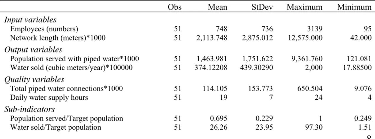
The model specification relies on two output measures: water supply service coverage (measured in terms of the population served with piped water) and the volumetric water sold. The latter is highly correlated with utility revenues that are supposedly reinvested in advancing (to new costumers) and maintaining (for existing customers) service coverage. Output increases are expected to positively influence utilities’ technical efficiency (and effectiveness). Table 1 presents some summary statistics. The data correspond to 21 African countries that are equivalent to about 60 percent of all countries whose urban WU managers or administrators responded to the WOP-Africa self assessment and benchmarking questionnaires by 2006.

On average, about 1,463,981 customers are served with piped water systems. The utility with the lowest customer coverage serves about 48 percent of its licensed target total population (about one twenty one thousand customers) while that with the highest coverage serves about 51 percent of its total population. The highest performing utility in this partial productivity dimension sells about 112 times more water than the lowest performing utility (see Table 1).

We consider two inputs: the total number of employees and the water distribution mains length (network length). The inputs capture utilities’ labor and capital expenditure, respectively. However, since the WOP dataset does not provide disaggregated employee categories (full or part time, technical or administrative), we use the aggregated employee count that implicitly assumes uniform skill distribution across observed WUs. The average utility employs 748 persons. The utility with the most employees hires about 3,139 persons while that with the lowest employees engages 95 persons. Among other capital input measures, water distribution network length is less prone to country-specific measurement and exchange rate incompatibilities. The utility with the longest piped water system built a water distribution main that is about 300 times longer than the utility with the shortest piped water system.

Table 1: African urban water utilities summary statistics, 2006

Obs Mean StDev Maximum Minimum

Input variables

Employees (numbers) 51 748 736 3139 95

Network length (meters)*1000 51 2,113.748 2,875.012 12,575.000 42.000 Output variables

Population served with piped water*1000 51 1,463.981 1,751.622 9,361.760 121.081 Water sold (cubic meters/year)*100000 51 374.12208 439.30290 2,000 17.88500 Quality variables

Total piped water connections*1000 51 114.105 153.773 650.504 9.076

Daily water supply hours 51 19 7 24 4

Sub-indicators

Population served/Target population 51 0.695 0.229 1 0.249 Water sold/Target population 51 26.26 23.95 97.30 1.51

9

Total water connections/Target population 51 0.081 0.086 0.307 0.004 Environmental variables

Independent regulation (IR, dummy) 51 0.294 0.460 1 0 Performance contract use (PC, dummy) 51 0.628 0.488 1 0

GDP 51 0.257 0.269 1 0.051

Network density 51 0.065 0.049 0.286 0.015

Abbreviations: Obs: Observations; StDev: Standard deviation; GDP: Gross domestic product per capita purchasing power parity; Network density: Total piped water connections per unit network length.

In addition to this basic model (hereafter referred to as Model 1), we consider different output quality variables. Previous literature (see Annex 1) considered the latter in the form of chemical treatment tests (Antonioli and Filippini, 2001; Corton, 2003; Lin, 2005; Lin and Berg, 2008), quality indexes (Saal and Parker, 2000: 2001; Woodbury and Dollery, 2004; Erbetta and Cave, 2007; Bottasso and Conti, 2009), service coverage (Lin, 2005), service continuity (Corton, 2003; Lin, 2005; Lin and Berg, 2008), accounted-for water ratio (Lin, 2005), unaccounted-for water (Antonioli and Filippini, 2001; Garcia and Thomas, 2001; Tupper and Resende, 2004; Picazo-Tadeo et al., 2008), annual mains breakage per observed output (Bhattacharyya et al., 1994), bathing water intensity (Saal et al., 2007) and household ratio (Mizutani and Urakami, 2001). This paper captures utilities-output quality in terms of services connectivity and continuity. We use the total active piped water connections to proxy the former. Earlier WU efficiency studies have treated water connections variedly. Assuming a cost minimization objective, utilities’ water connections have previously been used as a proxy for capital input (see Estache and Kouassi, 2002; Lin, 2005; Lin and Berg, 2008), utilities output (see Ashton, 2000a: 2000b; Estache and Rossi, 2002; García-Sánchez, 2006; Saal et al., 2007), operational scale (see for example Erbetta and Cave, 2007) and to capture the impact of utilities operational environment on cost efficiency (see for example Teeples and Glyer, 1987).

Holding inputs fixed we argue that to supply non-contaminated water, piped water distribution systems matter. This is importantly so for regions like Africa where universal urban water services coverage and increased mortality rates (owing especially to high water borne/water related diseases) are key developmental challenges. Using the case of India, Jalan and Ravallion (2003) found piped water delivery positively and significantly associated with reduced prevalence and duration of water borne diseases (e.g., diarrhea). As the safety of alternative urban non-piped water distribution systems is not always guaranteed and can consequently accrue costs to affected customers, we use dissimilar to earlier studies, the number of active piped water connections as a proxy for utilities output quality.

To capture services continuity, we use utilities daily hours of service provision. For connected customers, however, utilities can only provide water supply services for a maximum of 24 hours.

10

As such, the variable is by construction restricted (between 0 and 24). To avoid imposing such a restriction to the DEA linear program, we adjust the output quality variable to take into account hours of daily water supply per connection. We therefore use the product of the daily hours of service provision and total piped water connections to capture utilities’ service continuity. We consider service connectivity as a quality variable in Model 2. The smallest performing WU makes 9076 piped water connections (serving about 742,000 customers). This is 72 times less than the utility with the highest number of connections (650,504 but serving about 4,134,000 customers) within its licensed jurisdiction.

Model 3 includes service continuity. Constant service continuity for connected customers is associated with improved public health among other socio-economic advancements. The average observed utility provides daily piped water services over 19 hours (see Table 1).

3.2 Environmental variables

Often, urban WUs fail to reach their performance targets due to country specific (e.g., national income), sector specific (e.g., adopted regulatory structure) and/or utility specific (e.g., customer density) factors. In an attempt to explain this inability, we identify four environmental factors that potentially influence utilities’ performance (technical efficiency and/or effectiveness). First, urban water supply is highly capital intensive. The lower the national per capita income, the lower the abilities to pay for public services, the less accrued returns are allocated for capital (re)investment and, the more exclusive water service provision becomes. Wealthier economies are more likely to (i) subsidize water infrastructure investments and (ii) maintain strong regulatory institutions (Franceys and Gerlach, 2008). To capture these country-specific differences, we use the gross domestic product per capita purchasing power parity (hereafter, GDP) indicator (WDI and GDF, 2010). Across observed countries, GDP is on average 3,431$ (i.e., 25.7 percent7_{, see Table 1). Gabon is the wealthiest country (GDP = 13,349$) in the sample,} while Malawi is the poorest with a GDP value of 681.37$.

Second, regulation (largely economic regulation) is often adopted in the form of either formal (licenses) or informal (sector-specific commitments) rules. Strict regulatory systems (in the form of independent regulation) potentially results in increased regulatory risks (new expensive standards, tariffs) or sector credibility that respectively, augment sector uncertainty or/and investments (Kirkpatrick et al., 2006). The WOP-Africa dataset distinguishes two main types of utilities: those regulated by an independent regulator and those regulated by the use of performance contracts (WSP-WB, 2009). In Africa, independent regulatory structures are commonly established solely for the water sector (e.g., in Kenya, Mozambique and Zambia) or

7 _{Countries GDPPPP values are normalized (as a share of the maximum GDPPPP value across observed African}

11

conjointly with other sectors including energy, telecommunications, waste removal and gas development sectors for example in Burundi, Gabon, Gambia, Ghana, Madagascar, Mali, Niger, Tanzania and Rwanda (see MWI, 2002; NWASCO, 2004; Oelmann, 2007; Osumanu, 2008; URT, 2009; Mwanza, 2010). By 2006, about 29 percent of the observed urban water sectors in Africa had adopted independent regulatory institutions (see Table 1).8

Regulation by contracts (e.g., in Burkina Faso, Ethiopia, Gabon and Senegal) is commonly organized within a ministerial department or an asset holding agency and overseen by an independent committee (AfDB-WPP, 2010; MWR, 2001). About 63 percent of the observed urban water sectors had introduced regulation by performance contracts by 2006 (see Table 1). We use two dummy variables (i) independent regulation and, (ii) performance contract use to capture these potential reverse causalities between utilities performance and regulatory strictness (at the sector level).

Thirdly, among other ways by which WUs can respond to customer demands for increased quality services provision is by augmenting the number of customers (population served) per mains length. Nonetheless, since all observed utilities provide services to urban populations that are more or less homogeneously populated (per square kilometer), we consider the influence of utilities’ network densities (rather than customer densities) on their performance. To capture these network density economies at the utility level, we use the number of piped water connections per unit network length. On average, most observed WUs in Africa connect 6.5 percent of their population per unit network length. The smallest performing WU makes about 1.5 percent water connections per its established piped water distribution system (see Table 1).

3.3 Stepwise model

In assessing utilities’ performance, we define a step-wise empirical model consisting of four steps. In step 1, we estimate utilities’ technical efficiency (output expansion) under given resource constraints. Here, we rely on the input and output variables detailed in section 3.1 and the DEA-VRS model outlined in section 2.

Given unit input on one hand, utility managers seek to attain various effectiveness targets within their licensed service areas. They are supposed to serve as many customers with quality water systems, sell as much water, connect as many customers and provide reliable services for connected customers. Across observed WUs, 70 percent of the target population within utilities

8 _{Mwanza (2010) advocates for the creation of independent statutory regulatory agencies in Africa based on (i) clear}

legislative frameworks free from ministerial control, (ii) transparent procedures for appointing the board of directors, commissioners and key staff, (iii) secure tenure for elected oversight members remunerated based on private salary structures, (iv) sustainable finances through a regulatory fee charged on the regulated utilities, and (v) depolicized reporting mechanisms for the elected oversight members.

12

licensed jurisdictions are served with quality water supply systems (see Table 1). On average, observed utilities are able to sell about 26 cubic meters of water per customer per annum (though some water is often lost along the distribution system) and make about 81 connections by 1,000 inhabitants (see Table 1). To meet these effectiveness goals for all customers within their licensed jurisdictions, utility managers need not only to perform better in one of the targets, but in all of them.

To aggregate the different effectiveness targets, one can use the prices of the sub-indicators as weights. In addition (or alternatively), one could seek experts’ opinion on the exact significance attached to all identified sub-indicators. Such price and/or subjective value information can then be used in defining the lower and upper bounds between which each of the identified sub-indicator can be allowed to vary. This kind of aggregation helps to enhance the resultant performance indexes’ discriminatory power, credibility and acceptability among related sector stakeholders. Thanassoulis et al. (2004) and Nardo et al. (2005) provide an overview of diverse aggregation techniques.

For most public service sectors however, only sub-indicator’s quantitative information is (consistently) available. In other cases, it is not a guarantee that a consensual point is attained regarding the exact sub-indicator’s weights (Cherchye et al., 2007). To avoid such risks, we rely in a second step, on the BoD weighting approach (Cherchye et al., 2007). The BoD framework allows each utility to freely (and endogenously) choose non-negative weights for all selected sub-indicators that maximize its eventual effectiveness performance relative to other observed utilities. As such, specific utilities’ poor performance can only be blamed on the particular self-selected BoD weights rather than on some a priori defined (often unfair or non-consensual, etc) sub-indicator weighting system (Shwartz et al., 2010). By construction, resultant performance indexes (bounded between 0 and 1) only reflect utilities ‘achievement’ given unit input9 _{- that is,} “without explicit reference to the inputs that are used in achieving such performance” (Cherchye et al., 2007). BoD values of one imply 100 percent effectiveness while values near to (far from) one denote high (or low) effectiveness, relative to the benchmark utilities located on the best-practice effectiveness frontier.

On the other hand and due to inefficiencies, utilities could fail to attain 100 percent effectiveness. Or vice versa, ineffective supply could foster a higher efficiency. To examine this relationship we use in a third step, the ratio of utilities’ effectiveness (BoD) by technical efficiency (TE). We refer to this ratio as the utilities ‘Potential Input Capacity’ (PIC).

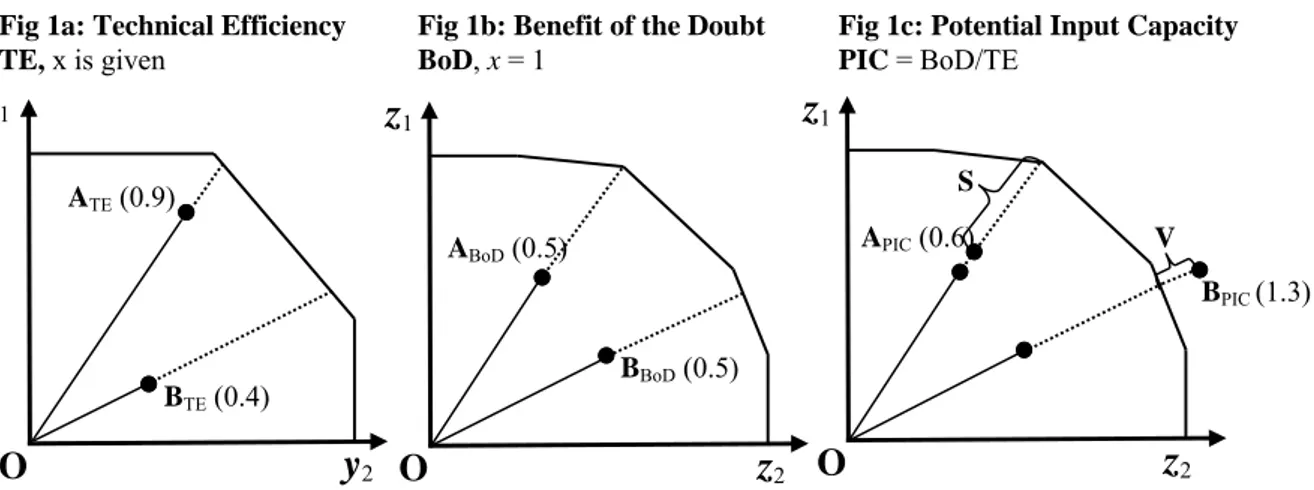
Consider in Figure 1 (i.e., Fig 1a to1c) utilities ‘A’ and ‘B’. Figure 1a presents the technical efficiency of the observations. It is presented in an output-oriented framework where we

13

normalized the inputs. Observation ‘A’ is clearly more efficient than observation ‘B’, although not as efficient as its best practice. Therefore, observation ‘A’ and ‘B’ are located below the best practice frontier. Figure 1b presents the effectiveness of the two observations. Here, the outputs are presented relatively to the unit input (i.e., the BoD framework). Both observations are as effective.

Figure 1c presents the PIC ratio. The ratio of effectiveness to technical efficiency equals to the distances OABoD/OATE and OBBoD/OBTE, respectively for ‘A’ and ‘B’. This ratio is denoted, respectively, by the distances OAPIC (utility A) and OBPIC (utility B), see Fig 1c. Given a priori defined output target (to serve all the target population within each utilities’ jurisdiction), the ratio indicates to what extent utilities potentially use available input resources (capital, labor, etc) to reach the target.

PIC values of less than one indicate resources deficiency. Affected utilities need more input resources to attain 100 percent effectiveness (reflected by the distance S for utility A in Fig 1c). For utilities with a PIC value < 1, ineffectiveness is a more serious issue than inefficiency. PIC values larger than one denote utilities’ excess use of resources. That is, if the specific utilities were technical efficient, they would reach their targets with less input resources (reflected by the distance V for utility B in Fig 1c). For these utilities with PIC > 1, inefficiency is a larger problem than ineffectiveness. PIC values equal to one indicate exact resource allocation for observed utilities. That is, if observed utilities are technical efficient, then they are also 100 percent effective.

Abbreviations: TE, x, BoD, PIC and y: As earlier defined; z: Variable representing the ratio of population

served and volumetric water sold over target population (see Section 3.3).

Fig 1a: Technical Efficiency TE, x is given

Fig 1b: Benefit of the Doubt BoD, x = 1

Fig 1c: Potential Input Capacity PIC = BoD/TE ATE (0.9) BTE (0.4)

O

y

2

y

1

z

2

O

z

1 APIC (0.6) V BPIC (1.3) S ABoD (0.5) BBoD (0.5)

O

z

2

z

1

14

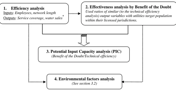
In a fourth and final step, we explore different inefficiency and ineffectiveness determinants. Unlike earlier studies that relied on the traditional two-step approach (where an environmental variable is regressed on the estimated efficiency scores), we use the double bootstrap procedure such that we correct for the measurement bias in the estimates (see Simar and Wilson, 2007 for an extensive discussion). Note that this fourth step allows us to indicate correlations between efficiency, effectiveness and environmental variables. Although not explicitly stated below, this does not allow us to draw causal interpretations. Figure 2 illustrates the four steps.

Figure 2: Urban water utilities performance - stepwise analytical framework

4

Water utilities efficiency and effectiveness

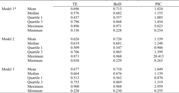
Table 2 presents the results of the analyses. Through the three model specifications (see section 3.1), utilities are observed to be more effective than efficient. On average, technical efficiency across the three model specifications amounts to 70% (when no output quality variables are considered), 63% (when service connectivity variables are considered) and 68% (when service continuity variables are considered). Effectiveness amounts in the three specifications to 71%, 73% and 71%, respectively. A quarter of the observed utilities have the possibility to increase their effectiveness by 44 percent and technical efficiency by 51 percent. The latter, through the three model specifications, is equivalent to about 56 (Model 1), 49.1 (Model 2) and 48.8 (Model 3) percent. This implies that, when a quarter of the observed utilities is considered, utilities are

* Besides this basic model specification, two output quality (service connectivity and adjusted service continuity) variables are considered respectively, in Models 2 and 3 (see Section 3.1).

1. Efficiency analysis

Inputs: Employees, network length Outputs: Service coverage, water sales*

2. Effectiveness analysis by Benefit of the Doubt

Used ratios of similar (to the technical efficiency analysis) output variables with utilities target population within their licensed jurisdictions.

3. Potential Input Capacity analysis (PIC)

(Benefit of the Doubt/Technical efficiency)

4. Environmental factors analysis

15

found to be less technical inefficient and ineffective only when service continuity quality variables are considered.

As the average hides some information, we focus on the different quartiles of the efficiency distribution. In model 1, technical efficiency of the third quartile amounts to 80%. This decreases to 71% in model 2 and to 76% in model 3. However, effectiveness results do not show this pattern. Utilities effectiveness stays around 87% in all the three model specifications.

From the potential input capacity levels (PIC), we learn that the utilities (across the three model specifications) face more inefficiency than ineffectiveness problems. This implies that, if observed utilities would have been technical efficient, they would attain 100 percent effectiveness with less resources (inputs). As such, they do not need any additional resources to reach their effectiveness targets but a reduction of their existing inputs. The latter corresponds to about 2.4 percent (Model 1), 15.9 percent (Model 2) and 4.9 percent (Model 3). Note that, these PIC estimates are based on the underlying mean values thus, they do not necessarily correspond to the ratio of estimated TE and BoD means.

Across the three model specifications, technical efficiency is positively and significantly correlated with effectiveness only in the model without output quality variables (correlation of .29, p-value 0.0369) and if service continuity quality variables are considered (.44, p-value 0.0014). While the relation is not very strong, an increase in technical efficiency is potentially allied with an increase in effectiveness.

Table 2: Utilities technical efficiency, effectiveness and potential input capacity estimates

TE BoD PIC Model 1* Mean 0.696 0.713 1.024 Median 0.576 0.682 1.155 Quartile 1 0.437 0.557 1.005 Quartile 3 0.796 0.868 1.454 Maximum 0.896 0.971 5.023 Minimum 0.156 0.228 0.254 Model 2 Mean 0.626 0.726 1.159 Median 0.619 0.681 1.248 Quartile 1 0.509 0.547 0.906 Quartile 3 0.706 0.885 1.399 Maximum 0.871 0.968 20.413 Minimum 0.038 0.229 0.263 Model 3 Mean 0.677 0.710 1.049 Median 0.664 0.676 1.139 Quartile 1 0.512 0.562 0.870 Quartile 3 0.755 0.869 1.319 Maximum 0.900 0.968 2.959 Minimum 0.220 0.230 0.255

TE: Technical efficiency; BoD: Effectiveness; PIC: Potential input capacity. All estimates are weighted by the population served. *For all models (1-3), similar 51 WUs are observed. Model 1 corresponds to network length and employees as inputs; and coverage and water sales as outputs. Models 2 and 3 add respectively, service connectivity and continuity as outputs to Model 1.

16

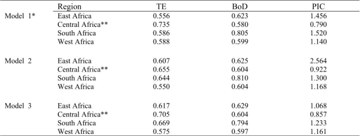
4.1 Regional performance

To identify regional patterns, we explore in Table 3 regional utility-performance differences. Across the three model specifications, East African urban WUs (such as from Ethiopia, Kenya, Tanzania, Uganda) are more technical inefficient than ineffective. Given their existing resources, these utilities can expand their outputs by 45 percent, 39 percent and 38 percent along model 1 to 3, respectively (see Table 3). Nonetheless, to entirely penetrate their licensed markets (i.e., completely attain their effectiveness targets for all population within their licensed jurisdictions) these utilities should increase their effectiveness (across the three model specifications) by 38 percent. Such performance improvement will demand no additional input usage (signaled respectively through the three models by PIC values of more than one).

Looking at both South African (including Malawi, Mauritius, Namibia, South Africa, Zambia) and West African (such as Benin, Cote d’Ivoire, Ghana, Mali, Mauritania, Nigeria) utilities, analogous conclusions are observed. Like their East African counterparts, these utilities seem less ineffective than technically inefficient. As indicated by their PIC values of more than one, observed utilities can indeed attain increased performance (100 percent effectiveness) with fewer resources than their present amounts. Input excess of about 35 and 16 percent across the three model specifications for the two regions respectively, is on average observed.

Through the three model specifications, South African utilities are the best performing - both in terms of effectiveness and technical efficiency. They are followed by (when only Models 2 and 3 results are considered) the East African and finally the West African utilities (see Table 3).

Table 3: Mean performance estimates per region

Region TE BoD PIC

Model 1* East Africa 0.556 0.623 1.456

Central Africa** 0.735 0.580 0.790

South Africa 0.586 0.805 1.520

West Africa 0.588 0.599 1.140

Model 2 East Africa 0.607 0.625 2.564

Central Africa** 0.655 0.604 0.922

South Africa 0.644 0.810 1.300

West Africa 0.550 0.604 1.168

Model 3 East Africa 0.617 0.629 1.068

Central Africa** 0.705 0.604 0.857

South Africa 0.669 0.794 1.233

West Africa 0.575 0.597 1.161

* For all models (1-3), similar 51 WUs are observed. TE, BoD and PIC: As earlier defined. ** Only one utility is observed per model. All estimates are weighted by the population served.

17

4.2 Explaining

utility

performance differences

To explain efficiency and effectiveness differences, the following specification is estimated (in a similar vein as in Simar and Wilson, 2007):

i density Network GDP PC IR i WUperf ₁ ₂ ₃ ₄ 

[4]

Where WUperfi denotes WUi’s performance in terms of efficiency or effectiveness, and



1

,

2

,

3

,

4 represent the estimated marginal effects on utilities’ performance of the regulation (independent or not - IR), the use of performance contracts (PC),10 _{gross domestic product per capita} purchasing power parity (GDP) and utilities network density.

The results are presented in Tables 4 and 5.11 _{Only countries’ GDP is found to positively and} significantly correlate to technical efficiency especially when service connectivity and continuity variables are considered (see Table 4). An increase by US$ 1,000 of a specific country’s GDP (say from US$ 2,420 to US$ 3,420) is significantly associated with a technical efficiency increase of 9.75 and 11.2 (i.e., when Models 2 and 3 results are considered, respectively). These particular findings are consistent with De Witte and Marques (2009). Using non-parametric envelopment techniques, the authors explored 122 urban WUs in Australia, Belgium, Netherlands, Portugal, United Kingdom (England and Wales) and found a positive correlation between utilities technical efficiency and regional wealth per capita (measured in gross regional product per capita).

The use of stricter regulatory systems (independent regulation) correlates positively with utilities’ technical efficiency.12 _{This is only significant when service connectivity variables are considered.} Previous literature provides mixed results on the correlation between utilities’ efficiency and the kind of adopted regulatory structure. Anwandter and Ozuna (2002) found an insignificant link between autonomous (independent) regulation and urban WUs efficiency. They observed a sample of 110 utilities in Mexico in 1995. Similar results were observed by Kirkpatrick et al. (2006) on a sample of 14 African urban WUs in 2000. On the other hand, and based on 211 and 10 urban WUs in Wisconsin and, England and Wales respectively, Aubert and Reynaud (2005) and Fabrizio and Martin (2007) found analogous positive and significant correlation between regulation and efficiency.13 _{In our case, a 1 percent increase in independent regulation is} significantly associated with a 9.7 percent increase in technical efficiency (i.e., when Model 2

10 _{We carefully examined the existence of any multicollinearity between regulation and the use of performance}

contracts, but found no evidence.

11 _{To examine the robustness of our results, we explored in different models the influences of additional}

country-specific (including political stability and corruption levels), sector-country-specific (such as, annual sector reports availability) and utility-specific (including utility ownership and scale economies) variables. While their influences are insignificant, estimated utility performance scores remain largely unchanged.

12 _{A sub-sample with either regulation or the use of performance contracts yields similar results.} 13 _{See also, Erbetta and Cave, 2007 and the reference therein.}

18

results are considered). Other control variables (use of performance contracts and network density) yield insignificant influences on utilities technical efficiency (see Table 4).

Table 4: Technical efficiency determinants

Variable Model 1** Model 2 Model 3

Constant 0.514 (0.082)*** 0.439 (0.063) *** 0.483 (0.067)*** Independent regulation (dummy) 0.015 (0.089) 0.097 (0.057) * 0.008 (0.070) Performance contract use (dummy) -0.045 (0.076) 0.043 (0.053) 0.026 (0.060)

GDP 0.197 (0.127) 0.236 (0.086)*** 0.271 (0.094)***

Network density 0.613 (0.759) 0.702 (0.604) 0.780 (0.502)

Note: Standard error between brackets; * and *** denote respectively, statistical significance at 10 and 1 percent. ** For all models (1-3), similar 51 WUs are observed. GDP and Network density as earlier defined.

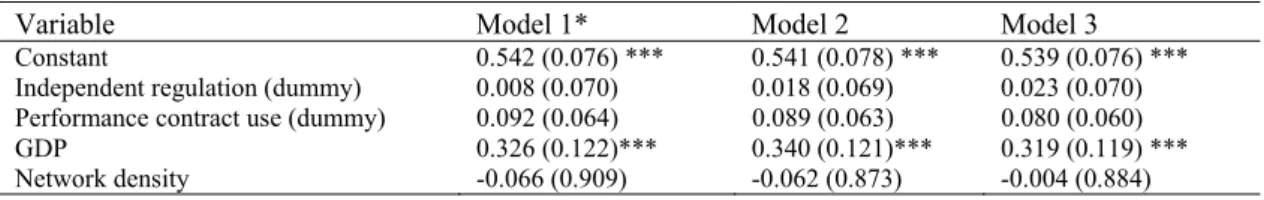
Repeating the double bootstrap procedure on the effectiveness scores yields slightly different estimates. The results are presented in Table 5. A 1% increase in countries’ GDP is positively and significantly linked to a more than 30 percent increase (on average across the model specifications) in utilities effectiveness. Interestingly, network density is found negatively correlated with utilities’ effectiveness. This finding is, however, insignificant through the three model specifications. Though lower influences (compared to the estimated influence on utilities technical efficiency) are on average observed across the three specifications of about 4.4 percent, higher network densities are found to be good for technical efficiency improvement, but at the expense of reduced effectiveness. This can especially be the case when customers are sparsely located across specific utilities’ licensed jurisdictions.

The remaining exogenous factors (independent regulation and use of performance contracts) are found to positively but insignificantly influence utilities’ effectiveness (see Table 5).

Table 5: Effectiveness determinants

Variable Model 1* Model 2 Model 3

Constant 0.542 (0.076) *** 0.541 (0.078) *** 0.539 (0.076) *** Independent regulation (dummy) 0.008 (0.070) 0.018 (0.069) 0.023 (0.070) Performance contract use (dummy) 0.092 (0.064) 0.089 (0.063) 0.080 (0.060)

GDP 0.326 (0.122)*** 0.340 (0.121)*** 0.319 (0.119) *** Network density -0.066 (0.909) -0.062 (0.873) -0.004 (0.884)

19

5

Conclusion and policy advice

This paper explored the use of benchmarking techniques in facilitating informed policy decisions across the African urban water sector. Using the double bootstrap procedure in a step-wise model approach, technical efficiency scores were first estimated and compared across different model specifications. The first (basic) specification ignored output quality variables. The second and third specification took into account both service connectivity (in terms of active piped water connections) and service continuity factors (measured in daily hours of water supply).

Second, a utility’s effectiveness levels were explored and unbundled from inefficiency in a third step. In the latter step, we used the ratio of utilities’ effectiveness to technical efficiency to understand the key reasons behind utilities poor performance (due to either inefficiency or ineffectiveness) and the extent to which observed utilities utilize available resources to reach their effectiveness targets. We referred to this ratio as the ‘potential input capacity’ (PIC). PIC values of less than, more than or equal to one denote utilities’ resources deficiency, excess use of input resources (due to higher inefficiency than ineffectiveness problems) and, exact resource allocation. Finally, possible influences of country, sector and utility-specific environmental variables on utilities’ technical efficiency (and effectiveness) levels were explored.

The results pointed out that most utilities faced more inefficiency than ineffectiveness problems (PIC values > 1). Consequently, if the utilities would have been performing as efficiently as the best practice observations, they would achieve their effectiveness targets with fewer resources. To provide water supply services to all the population within their licensed jurisdiction and attain 100 percent effectiveness, these utilities would not need any additional resources.

Across the African region, no major performance differences were observed. Utilities across the East, West and Southern African regions seemed less ineffective than technically inefficient. To fully penetrate their markets, these utilities would need to reduce their input use (as evident from their PIC values of more than one). Nonetheless, South African utilities are the most well performing (both effectively and efficiently) followed by (i.e., when both service connectivity and continuity variables are considered) the East African and the West African utilities.

Only countries’ economic development (measured in terms of the gross domestic product per capita purchasing power parity) is positively and significantly linked to utilities technical efficiency and effectiveness. Network density correlates positively to utilities’ technical efficiency but negatively influences utilities’ effectiveness. This is, however, insignificant across the three model specifications. Independent regulation is positively found linked to utilities’ technical efficiency and effectiveness. Nevertheless, this is only significant when service connectivity variables are considered.

20

Despite the fact that the paper been based on correlations and thus does not provide causal relationships, it offers some clear insights for policy. First, the paper confirms that efficiency and effectiveness are not a trade-off. Water utilities can improve their effectiveness by increasing their efficiency. To do so, they should learn from best practices. Second, utility regulators, managers and policy makers should carefully take into account both efficiency and effectiveness performance indicators. This paper provided one way of disentangling ineffectiveness from inefficiency. Lastly, national economic advancement matters for utilities’ efficiency and effectiveness improvement. International organizations such as the World Bank and the United Nations should thus foster the wealth of countries. This in turn will improve the efficiency and effectiveness of public service utilities.

We see various avenues of further research. First, the availability of complete operational data (both quantity and cost data) would permit the extension of this study to explore other kinds of efficiency (including cost and allocative efficiencies) and effectiveness measures. Second, despite this first study, a better understanding of the complex relationship between efficiency and effectiveness is needed. Therefore, it would be insightful to apply the proposed step-wise model to other sectors and other continents. Third, the paper at hand provides some first steps in explaining the drivers of effectiveness. Further research is needed to explore the influence of quality indicators, political economy variables as well as management structures. A final promising avenue for further research consists of extending the cross-sectional setting to panel data. This should allow for controlling of country and utility fixed effects.

21

References

AfDB-WPP (African Development Bank Water Partnership Program). (2010). Water sector governance in Africa: Theory and practice (Vol. 1). Tunis, Tunisia: African Development Bank Water Partnership Program.

Antonioli, B., and Filippini, M. (2001). The use of a variable cost function in the regulation of the Italian water industry. Utilities Policy, 10(3-4): 181-187.

Anwandter, L., and Ozuna, T. (2002). Can public sector reforms improve the efficiency of public water utilities? Environment and Development Economics, 7(04): 687-700.

Ashton, J. (2000a). Total factor productivity growth and technical change in the water and sewerage industry. Service Industries Journal, 20 (4): 121–130.

Ashton, J. (2000b). Cost efficiency in the UK water and sewerage industry. Applied Economics Letters, 7 (7): 455-458.

Aubert, C., and Reynaud, A. (2005). The impact of regulation on cost efficiency: An empirical analysis of Wisconsin water utilities. Journal of Productivity Analysis, 23(3): 383-409.

Banker, D. (1984). Estimating most productive scale size using data envelopment analysis. European Journal of Operational Research, 17(1): 35-44.

Berg, S. (2007). Conflict resolution: benchmarking water utility performance. Public Administration and Development, 27(1): 1-11.

Bhattacharyya, A., Parker, E., and Raffiee, K. (1994). An examination of the effect of ownership on the relative efficiency of public and private water utilities. Land Economics, 70(2): 197-209. Bogetoft, P., and Otto, L. (2011). Benchmarking with DEA, SFA, and R. USA: Springer Science+Business Media, LLC.

Bottasso, A., and Conti, M. (2009). Price cap regulation and the ratchet effect: A generalized index approach. Journal of Productivity Analysis, 32(3): 191-201.

Charnes, A., Cooper, W., and Rhodes, E. (1978). Measuring the efficiency of decision making units. European Journal of Operational Research, 2(6): 429-444.

Cherchye, L., Moesen, W., Rogge, N and Puyenbroeck, T. (2007). An introduction to ‘Benefit of the Doubt’ composite indicators. Social Indicators Research, 82 (1): 111-145.

Coelli, T., Rao, P., O’Donnell, C., and Battese, G. (2005). An introduction to efficiency and productivity analysis (2nd ed.). USA: Springer.

Corton, M. (2003). Benchmarking in the Latin American water sector: the case of Peru. Utilities Policy, 11(3): 133-142.

Daraio, C., and Simar, L. (2007). Advanced robust and nonparametric methods in efficiency analysis: Methodology and applications. USA: Springer Science+Business Media, LLC.

22

De Witte, K., and Marques, R. (2009). Designing performance incentives, an international benchmark study in the water sector. Central European Journal of Operations Research, 18(2): 189-220.

Erbetta, F., and Cave, M. (2007). Regulation and efficiency incentives: Evidence from the England and Wales water and sewerage industry. Review of Network Economics, 6 (4): 425 – 452.

Estache, A., and Kouassi, E. (2002). Sector organization, governance, and the inefficiency of African water utilities (Policy Research Working Paper No. 2890), The World Bank.

Estache, A., and Rossi, M. ( How Different Is the Efficiency of Public and Private Water Companies in Asia? The World Bank Economic Review, 16 (1): 139 – 148.

Fabrizio, E., and Martin, C. (2007). Regulation and efficiency incentives: Evidence from the England and Wales water and sewerage industry. Review of Network Economics, 6(4): 425-452. Farrell, M. (1957). The measurement of productive efficiency. Journal of the Royal Statistical Society. Series A (General), 120 (3): 253-290.

Franceys, R., and Gerlach, E. (2008). Regulating water and sanitation for the poor: Economic regulation for public and private partnerships. United Kingdom: Earthscan Publications Ltd. Fried, H., Lovell, K., and Schmidt, S. (2008). The measurement of productive efficiency and productivity growth. USA: Oxford University Press.

Garcia, S., and Thomas, A. (2001). The structure of municipal water supply costs: Application to a panel of French local communities. Journal of Productivity Analysis, 16(1): 5 - 29.

García-Sánchez, I. (2006). Efficiency measurement in Spanish local government: The case of municipal water services. Review of Policy Research, 23(2): 355–372.

Greene, W. (2008). The econometric approach to efficiency analysis. In Fried, H., Lovell, C., and Schmidt., S, The measurement of productive efficiency and productivity growth (pp. 92 - 250). New York: Oxford University Press, Inc.

Jalan, J., and Ravallion, M. (2003). Does piped water reduce diarrhea for children in rural India? Journal of Econometrics, 112(1): 153–173

Kirkpatrick, C., Parker, D., and Zhang, Y. (2006). An empirical analysis of state and private-sector provision of water services in Africa. The World Bank Economic Review, 20(1): 143 -163. Kneip, A., Simar, L., and Wilson, P. (2003). Asymptotics for DEA estimators in nonparametric frontier models (Technical report No. 0323). IAP Statistics Network. Interuniversity Attraction Pole, Belgium.

Kneip, A., Simar, L., and Wilson, P. (2008). Asymptotics and consistent bootstraps for DEA estimators in nonparametric frontier models. Econometric Theory, 24(06): 1663-1697.

23

Lin, C. (2005). Service quality and prospects for benchmarking: Evidence from the Peru water sector. Utilities Policy, 13(3): 230-239.

Lin, C., and Berg, S. (2008). Incorporating service quality into yardstick regulation: An application to the Peru water sector. Review of Industrial Organization, 32(1): 53-75.

Lovell, K., Jesus, P., and Judi, T. (1995). Measuring macroeconomic performance in the OECD: A comparison of European and non-European countries. European Journal of Operational Research, 87 (3): 507-518.

Madhoo, Y. (2007). International trends in water utility regimes. Annals of Public and Cooperative Economics, 78(1): 87-135.

Melyn, W., and Moesen, W. 1991. Towards a synthetic indicator of macroeconomic performance: Unequal weighting when limited information is available. Public Economics Research Paper 17, K.U.Leuven Centrum voor Economische Studiën, Belgium.

Mizutani, F., and Urakami, T. (2001). Identifying network density and scale economies for Japanese water supply organizations. Papers in Regional Science, 80(2): 211–230.

MWI (Ministry of Water and Irrigation). (2002). Water Act, No 8. Republic of Kenya.

Mwanza, D. (2010). Roles and institutional arrangements for economic regulation of urban water services in Sub-Saharan Africa (Doctoral thesis). Loughborough University, United Kingdom. MWR (Ministry of Water Resources). (2001). Ethiopian water sector policy. The Federal Democratic Republic of Ethiopia: Ministry of Water Resources.

Nardo, M., Saisana,M., Saltelli, A., Tarantola, S., Hoffman, A., and Giovannini, E. (2005). Handbook on constructing composite indicators: Methodology and user guide. OECD Statistics Working Paper 2005/03, OECD Publishing.

NWASCO (National Water Supply and Sanitation Council). (2004). Water sector reform in Zambia. The Republic of Zambia: National Water Supply and Sanitation Council.

Oelmann, M. (2007). Assessment of the current regulatory practices of the Southern and East African water utilities regulators (Synthesis report of a meeting of African water utilities regulators). Lusaka, Zambia.

Osumanu, I. (2008). Private sector participation in urban water and sanitation provision in Ghana: Experiences from the Tamale Metropolitan Area (TMA). Environmental Management, 42(1): 102-110.

Pestieau, P., and Tulkens, H. (1993). Assessing and explaining the performance of public enterprises”, FinanzArchiv/Public Finance Analysis, 50 (3): 293-323.

Picazo-Tadeo, A., Sáez-Fernández, F., and González-Gómez, F. (2008). Does service quality matter in measuring the performance of water utilities? Utilities Policy, 16(1): 30-38.

24

Saal, D., and Parker, D. (2000). The impact of privatization and regulation on the water and sewerage industry in England and Wales: a translog cost function model. Managerial and Decision Economics, 21(6): 253-268.

Saal, D., and Parker, D. (2001). Productivity and price performance in the privatized water and sewerage companies of England and Wales. Journal of Regulatory Economics, 20(1): 61 - 90. Saal, D., Parker, D., and Weyman-Jones, T. (2007). Determining the contribution of technical change, efficiency change and scale change to productivity growth in the privatized English and Welsh water and sewerage industry: 1985–2000. Journal of Productivity Analysis, 28(1): 127 - 139.

Saisana, M., and Tarantola, S. (2002). State-of-the-art report on current methodologies and practices for composite indicator development. Institute for the Protection and Security of the Citizen Technological and Economic Risk Management, EC Joint Research Centre, Italy.

Simar, L., and Wilson, P. (2007). Estimation and inference in two-stage, semi-parametric models of production processes. Journal of Econometrics, 136(1): 31-64.

Shwartz, M., Burgess, J., and Berlowitz, D. (2010). Benefit-of-the-doubt approaches for calculating a composite measure of quality. Health Services and Outcomes Research Methodology, 9(4): 234-251.

Teeples, R., and Glyer, D. (1987). Cost of water delivery systems: specification and ownership effects. The Review of Economics and Statistics, 69 (3): 399-408.

Thanassoulis, E., Portela, M., and Allen, R. (2004). Incorporating Value Judgments in DEA. In Cooper, W., Seiford, L., and Zhu, J, Handbook on Data Envelopment Analysis, Boston: Kluwer Academic Publishers.

Tupper, H., and Resende, M. (2004). Efficiency and regulatory issues in the Brazilian water and sewage sector: An empirical study. Utilities Policy, 12(1): 29-40.

UNESCO., and Earthscan. (2009). Water in a changing world: The United Nations world water development report 3. Paris, France and London, United Kingdom: United Nations Educational Scientific and Cultural Organization and Earthscan publishing.

URT (United Republic of Tanzania). (2009). The water supply and sanitation Act, No. 12. Dar Es Salaam, The United Republic of Tanzania.

UNSGAB (United Nations Secretary-General’s Advisory Board). (2006). Hashimoto action plan: Compendium of actions. United Nations Secretary-General’s Advisory Board on Water and Sanitation.

WDI (World Development Indicators)., and GDF (Global Development Finance). (2010). GDP per capita, PPP (current international $).

http://search.worldbank.org/quickview?name=GDP+per+capita%2C+PPP+%28current+internati onal+%24%29&id=NY.GDP.PCAP.PP.CD&type=Indicators&qterm=purchasing+power+parity, Accessed June 2010.

25

WHO (World health Organization)., and UNICEF (The United Nations Children's Fund). (2000). Global water supply and sanitation assessment 2000 report. USA: World Health Organization and United Nations Children’s Fund.

Woodbury, K., and Dollery, B. (2004). Efficiency measurement in Australian local government: The case of New South Wales municipal water services. Review of Policy Research, 21(5): 615-636.

WSP-WB (Water and Sanitation Program-Africa of the World Bank). (2009). Water operators partnership: Africa utility performance assessment. Nairobi, Kenya: The World Bank/UN Habitat/ESAR/AfWA.

Yatchew, A. (1998), Nonparametric regression techniques in economics. Journal of Economic Literature 36 (2): 669-721.

26

Annex 1: Quality variables used in urban water distribution efficiency studies

Author Urban WUs (period, place) Technique Quality variable used Quality variable influence on efficiency

Bhattacharyya et al., 1994 257 (1992, North America) TGV cost function Mains breakdowns/output/year Increased inputs requirement Saal and Parker, 2000 10 (1985-1999, England and Wales) MO translog cost function 9 water quality measures* Quality-driven scope economies

Antonioli & Filippini, 2001 32 (1991-1995, Italy) CD variable cost function Water losses, WSCtreatment Only WSCtreatment increases variable costs Garcia & Thomas, 2001 55 (1995-1997, France) GMM, translog cost function Network losses Increased input requirement

Saal & Parker, 2001 10 (1985-1999, England and Wales) Tornqvist indexes 9 water quality measures* Lower productivity post-privatization Mizutani & Urakami, 2001 112 (1994, Japan) Log-linear, translog, hedonic function Purifier level, household ratio Better network and scale economies capture Corton, 2003 44 (1996-1998, Peru) Regression techniques CL tests, SCty, WSCtreatment No significant impact on operation costs Tupper & Resende, 2004 20 (1996–2000, Brazil) DEA with tobit regression Water loss index Positive significant influence Woodbury & Dollery, 2004 73 (1998-2000, Australia) DEA with tobit regression Water quality** & service*** indexes Minor variations in utilities efficiency Lin, 2005 198 (1996-2001, Peru) Stochastic cost frontier AW ratio, CL tests, SCv, SCty Positive significant influence Saal et al., 2007 10 (1985-2000, England and Wales) GPP index Bathing water intensity Increased input requirement Erbetta & Cave, 2007 10 (1993-2005, England and Wales) DEA, Stochastic frontier WU-specific DWQCI Better output caputure Lin & Berg, 2008 38 (1996-2001, Peru) DEA, PSM and QMPI CL tests & SCty Positive influence Picazo-Tadeo et al., 2008 38 (2001, Spain) Translog cost function Unaccounted-for water Positive influence

Bottasso and Conti, 2009 10 (1995-2004, England and Wales) Translog cost function Water quality Lower productivity post-privatization

*identified by Ofwat as key for aesthetic, health and cost-effectiveness reasons; **compliance with chemical, physical and microbiological requirements; ***constituting water quality and service complaints and, the average customer outage; WUs: Water utilities; TGV: Translog generalized variable; MO: Multiple output; CD: Cobb-Douglas; GPP: Generalized parametric productivity; DEA: Data envelopment analysis; CL tests: positive rate of chlorine tests; SCty: Service continuity; WSCtreatment: Water served receiving chemical treatment (percentage); GMM: Generalized method of moments; AW ratio: Accounted-for water ratio; SCv: Service coverage; DWQCI: Drinking water quality compliance index as defined by the Drinking Water Inspectorate and the Environment Agency in the UK; PSM: Preference structure model; QMPI: Quality-incorporated Malmquist Productivity index